
 ?Mathematical formulae have been encoded as MathML and are displayed in this HTML version using MathJax in order to improve their display. Uncheck the box to turn MathJax off. This feature requires Javascript. Click on a formula to zoom.
Abstract
The aim of this paper is to introduce a formulation of linear programming problems involving intuitionistic fuzzy variables. Here, we will focus on duality and a simplex-based algorithm for these problems. We classify these problems into two main different categories: linear programming with intuitionistic fuzzy numbers problems and linear programming with intuitionistic fuzzy variables problems. The linear programming with intuitionistic fuzzy numbers problem had been solved in the previous literature, based on this fact we offer a procedure for solving the linear programming with intuitionistic fuzzy variables problems. In methods based on the simplex algorithm, it is not easy to obtain a primal basic feasible solution to the minimization linear programming with intuitionistic fuzzy variables problem with equality constraints and nonnegative variables. Therefore, we propose a dual simplex algorithm to solve these problems. Some fundamental concepts and theoretical results such as basic solution, optimality condition and etc., for linear programming with intuitionistic fuzzy variables problems, are established so far. Moreover, the weak and strong duality theorems for linear programming with intuitionistic fuzzy variables problems are proved. In the end, the computational procedure of the suggested approach is shown by numerical examples.
1. Introduction
Linear Programming is a branch of science in operations research field which has many different applications. Parameters and values of an LP model should be accurate in a primal one. However, in the real world, this assumption does not coincide with the reality. Some sort of uncertainty about the parameters might exist in the problems that we ought to deal with in our daily lives. In these cases, parameters of LP problems would be presented in fuzzy numbers. Application of fuzzy numbers in mathematical programming has a profound history. Zadeh [Citation1] was the first mathematician who proposed the Fuzzy Sets (FSs) theory for the first time. The notion of mathematical programming in the fuzzy environment was suggested by Tanaka et al. [Citation2] in the fuzzy decision-making frame for the first time which had been presented by Bellman and Zadeh [Citation3]. Noori-eskandari and Ghaznavi [Citation4] proposed an efficient algorithm for solving FLP problems. They consider some well-known approaches for solving FLP problems. They present some of the difficulties of these approaches and then, crisp LP problems are suggested for solving FLP problems. Linear programming problem in this environment, which is known as Fuzzy Linear Programming (FLP), was firstly investigated by Zimmerman [Citation5]. Nasseri and Ebrahimnejad [Citation6] proposed a novel approach to duality in FLP. Ghaznavi et al. [Citation7] introduced parametric analysis in Fuzzy Number Linear Programming (FNLP) problems. They considered the problem variations by using a linear ranking function. They used the fuzzy primal simplex method, the fuzzy dual simplex method and the fuzzy primal – dual simplex method to find the new optimal basis. For solving FLP problem, Mahdavi-Amiri et al. [Citation8] introduced the simplex algorithm of fuzzy primal. Also, other research has been done in this field, which is mostly based on comparing fuzzy numbers [Citation9,Citation10]. In other words, the ranking functions play a fundamental key role in the decision-making process [Citation11–14].
Later scientists faced with some problems that the FS theory was unable to have an answer for these problems, among them, Atanassov [Citation15] was the first scientist who presented a generalisation of FS theory to overcome to this obstacle which is known as Intuitionistic Fuzzy Set (IFS). The Degree of Membership (DM) and the Degree of Non-Membership (DNM) were applied to clarify the concept of the IFS theory. The only significant difference between the two theories is that in the FS theory, the summation of the DM of fuzzy numbers and Its complementary, the DNM
,which are numbers in the interval of [0,1] is equal to 1 whereas about the IFS theory, in addition to those two mentioned concepts there exist another concept in the same interval which is called the degree of doubt in order to have the same result as summation of 1. Similar to fuzzy numbers, the ranking of Intuitionistic Fuzzy Numbers (IFNs) plays an essential role in decision process. Nagoorgani et al. [Citation16] defined a ranking using score function based on
method. Seikh et al. [Citation17] introduced a method to approximate the IFNs of the triangular type, which we show here with TIFN. More recently, Atalik and Senturk [Citation18] proposed a new approach using the gergonne point to rank Triangular Intuitionistic Fuzzy Numbers (TIFNs). Suresh et al. [Citation19] introduced the ranking of TIFNs by means of magnitude and solved the intuitionistic FLP problems using this ranking. There are many other methods for ranking IFNs, that we refer to [Citation20–25]. Angelov [Citation26] studied the application of IFS to optimisation problems and proposed a solution approach to these problems. Sanny Kuriakose et al. [Citation27] suggested a non-membership function for the IFLP problem. A new form of LP problems in the intuitionistic fuzzy environment can be seen in the research of Parvathi et al. [Citation28,Citation29]. Ejegwa et al. [Citation30] presented a review paper on some definitions, basic operators, some algebras, etc., on intuitionistic FS. Dubey and Mehra [Citation31] proposed an approach based on the value and ambiguity of the index to solve linear programming problems with TIFNs. Nagoorgani and Ponnalagu [Citation32] studied the intuitionistic FLP problem methods using the intuitionistic fuzzy dual simplex method, in which the objective function can be maximise or minimise and also the constraints can be equal or unequal. Nasseri and Goli [Citation33] presented a method for solving fully intuitionistic FLP problems. They use the sign distance between IFNs for their comparison and then proposed an algorithm for finding the optimal solution. Nagoorgani and Ponnalagu [Citation34] used interval arithmetics to solve the intuitionistic FLP problems. Nachammai and Thangaraj [Citation35] solved the intuitionistic FLP problem based on special indexes that convert any IFN to a set of real numbers. Hepzibah and Vidhya [Citation36] and Sidhu [Citation37] studied on symmetric trapezoidal intuitionistic fuzzy numbers (TrIFNs). After defining a ranking function and arithmetic operations on these numbers, they solved the intuitionistic FLP problems without converting these problems into the crisp linear programming problem. Nasseri et al. [Citation38] proposed an approach for solving FLP problems based on comparison of IFNs by the help of linear accuracy function. They define an auxiliary problem, having only triangular intuitionistic fuzzy cost coefficients, and then study the relationships between these problems leading to a solution for the primary problem. Then, they develop intuitionistic fuzzy primal simplex algorithms for solving these problems. Prabakaran and Ganesan [Citation39] introduced Duality Theory for Intuitionistic FLP Problems. They discuss about the solution procedure of primal and dual LP problems involving IFNs without changing in to classical LP problems and then by using new type of arithmetic operations between IFNs, they have proved the weak and strong duality theorems. Sidhu and Kumar [Citation40] proposed mehar methods to solve intuitionistic FLP problems with trapezoidal intuitionistic fuzzy numbers. Ramik and Vlach [Citation41] introduced the intuitionistic FLP problem and then expressed the concepts of duality and related theorems. Now, we consider a minimisation IFVLP problem with equality constraints and nonnegative variables. Here we establish duality results and complementary slackness conditions for IFVLP problems. Then, for solving these problems, we develop the dual simplex method for IFVLP problems that directly uses the primal simplex table. In this case, we utilise the ranking function that already introduced in [Citation19].
In what follows, these topics would be described:
Some of the basic concepts of IFS theory would be explained, in Section 2. In Section 3, we classify the IFLP problems into two main different categories: IFNLP problems and IFVLP problems. Then, some fundamental concepts and theoretical results related to IFVLP problem such as basic solution, optimality condition and, etc., are given. In Section 4, we will consider the dual of an IFVLP problem and then by ranking function that already introduced in Section 2, all the dual theorems and the results will be proved. In Section 5, we present numerical examples and finally we explain the result of our research in Section 6.
2. Definitions and Preliminaries
In this section, we introduce some preliminaries and notions including IFSs and TIFNs which are applied throughout this paper. For more details, we refer to [Citation19,Citation30,Citation40,Citation42–45].
2.1. TIFNs and Their Arithmetic Operations
An IFS relates to each member of the universe set
, DM
and DNM
such that:
Also, the value
is named the degree of hesitancy of x to
.
Definition 2.1:
An IFN in the set of real numbers
, is define as
where
and
such that
and four functions
are the legs of
and
with the functions
and
are non-decreasing continuous functions and the functions
and
are non-increasing continuous functions and is denoted by
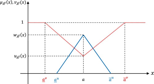
Definition 2.2:
A TIFN denoted by
, is a special IFN with the following DM and DNM, respectively:
where
. The value
represents the maximum DM and the value
represents the minimum DNM such that
and
(Figure 1).
Figure 1. A Triangular Intuitionistic Fuzzy Number.
Remark 2.1: Let us show the set of TIFNs as .
Let and
be two TIFNs and
, then
2.2. Ranking Function
Definition 2.3:
[Citation19] Assume that is a TIFN. We define magnitude as follows:
Assuming
we have
After simplification, we have
(1)
(1)
Definition 2.4:
Let and
be two TIFNs and
. Orders on
are defined as follows:
Also, throughout this paper, we let
as the zero TIFN.
In the following theorem, it is shown that in a special case, Mag is a linear ranking function. In fact, if we assume that the considered TIFNs have the same maximum DM and the same DNM, then Mag becomes a linear ranking function.
Theorem 2.1:
Let and
, be two TIFNs with
and
. Then:
Proof:
Let and
, be two TIFNs. Then for
, we have:
On the other hand, because
and
, so we have:
The same is true for
In this paper, we consider TIFNs in such a way that Mag be a linear ranking function.
Lemma 2.1:
Assume that Mag is the linear ranking function. Then
Proof:
(see [Citation46]).
Lemma 2.2:
Assume that Mag is the linear ranking function. Then
Proof:
(see [Citation46]).
3. Intuitionistic Fuzzy Linear Programming Problems
A crisp LP problem is as:
where the parameters
and
are given with crisp components and
is an unknown vector of variables to be found. Assume that some parameters are considered to be IFNs, then we obtain IFLP problem. In this section, we are going to consider them in details. Hence, based on their structures, we divide them into two main categories:
IFNLP problem,
IFVLP problems.
An IFNLP problem is defined as:
(2)
(2)
where
are given and
is to be determined. Also, Mag is the ranking function defined by (1).
An IFVLP problem is defined as:
(3)
(3)
where
and
are given and
is to be determined.
Definition 3.1:
The Intuitionistic Fuzzy (IF) vector is an IF feasible solution to (3) if
satisfies the constraints of Problem (3).
Definition 3.2:
An IF feasible solution is called an IF optimal solution for (3), if for all IF feasible solutions
for (3), we have
.
3.1. Intuitionistic Fuzzy Basic Feasible Solution
Here, we explain the notion of Intuitionistic Fuzzy Basic Feasible Solution (IFBFS) for IFVLP problem. Consider the following IFVLP problem:
(4)
(4)
where its parameters are defined as in (3). Let
and
. Partition
as
where
is an m × m, non-singular submatrix of
. Clearly,
. Assume that
be the solution to
where
is the
column of the coefficient matrix
. Obviously, the basic solution
(5)
(5)
is a solution of
The solution
, partitioned as
is called an Intuitionistic Fuzzy Basic Solution (IFBS) related to basis
. If
then the IFBS is feasible and the related IF objective value is
where
. Now, corresponding to any index
define
(6)
(6)
Obviously, for every basic index , it follows
, where
is the
unit vector. From
it follows:
(7)
(7)
Theorem 3.1:
(Optimality conditions). Suppose that the IFVLP problem (3) is non-degenerate and is a feasible basis. An IFBFS
is optimal to (3) iff
Proof:
Assume that is an IFBFS to (3), where
Therefore, the corresponding IF objective value is
(8)
(8)
Thus, from (9) we have:
(10)
(10)
Hence, for each IFBFS to (3), we have
Thus, from (7) and (8), we have
(11)
(11)
So, if we have
Then
and thus we get that
Therefore from (11) we see
hence,
is optimal.
Now, assume that is an optimal IFBFS to (3). For
from (7), we have
. From (11), it is obvious that if for some non-basic variable
we have
then this variable is a entering variable and
which is a contradiction to optimality of
. So, we have
.
4. Duality and the Main Results
In this part, we introduce the dual of an LP problem with IF variables (DIFVLP) and express the related dual results.
Definition 4.1:
For the primal IFVLP problem
(12)
(12)
the DIFVLP problem is formulated as:
(13)
(13)
4.1. Relations Between IFVLP and DIFVLP Problems
Theorem 4.1:
(Weak duality theorem)
Let and
be feasible solutions to IFVLP and DIFVLP problems, respectively. Then
Proof:
Since and
we have
On the other hand, since
and
we have
Now by using Lemma 2.1, we have
Corollary 4.1:
Suppose that and
are feasible solutions to IFVLP and DIFVLP problems, respectively, and
then
and
are optimal solutions for their corresponding problems.
Proof:
The proof is an obvious conclusion of Theorem 4.1.
Corollary 4.2:
Let one of the IFVLP or DIFVLP problems be unbounded, then the other one is infeasible.
Proof:
The proof is an obvious conclusion from the Theorem 4.1.
Theorem 4.2:
(Strong duality)
Suppose that one of the IFVLP or DIFVLP problems has an optimal solution, then its dual has an optimal solution, too. Also, their optimal IF objective values are equal.
Proof:
First, suppose that the IFVLP problem has an IF optimal solution, and . Suppose that
is the IF slack variables related to the constraints
The new equivalent problem to the IFVLP problem is as follows:
(14)
(14)
Suppose that is the optimal basic matrix and
is the IF basic optimal solution related to the IFVLP problem. By Theorem 4.1, we have
or equivalently,
Therefore, it follows that:
Now, assume that
Applying the preceding inequalities, we have
Hence,
is feasible for the DIFVLP problem and
and thus
Example 4.1:
Consider the following IFVLP problem as:
By the above discussion, the dual of this problem is as:
Theorem 4.3:
Consider a given IFLP problem and its dual. Only one of the statements (1) and (2) is true:
One of the primal or dual problems is unbounded and the other one is infeasible.
The primal problem and its dual have no feasible solution.
Proof:
(see [Citation46]).
Theorem 4.4:
(Complementary slackness theorem)
Assume that and
are feasible solutions to IFVLP problem and its DIFVLP problem, respectively. Then
and
are optimal iff
(15)
(15)
Proof:
Suppose that and
are feasible solutions for IFVLP problem and DIFVLP problem, respectively. Then
(16)
(16)
and
(17)
(17)
If we multiply by the inequality
we obtain
(18)
(18)
If we multiply
by the inequality
we obtain
(19)
(19)
Thus, we have
(20)
(20)
From optimality of and
for the primal and dual problems, we conclude
and using the relationship (20) we have
(21)
(21)
From (21) we will have
(22)
(22)
To prove the converse part of this theorem, we utilise the facts and
that imply
Thus, Corollary 4.1, results optimality of
and
.
4.2. The Dual Simplex Method
Here, we first introduce the dual simplex method to solve an IFVLP problem and then describe its algorithm.
Consider the following IFVLP problem as:
(23)
(23)
where the parameters of problem (23) are as introduced in (3).
We can rewrite (23) as:
(24)
(24)
where
We define
and
as:
(25)
(25)
Assume that for
we have
(26)
(26)
We define where
So, for
we have
Thus, from
it results that
Therefore,
(27)
(27)
Also, using (26), we have
and thus,
(28)
(28)
which results the dual feasibility. If
then we will have an IF feasible solution for the IFVLP problem. In addition, we have
Therefore, by Corollary 4.2, we obtain the optimality of
and
for the IFVLP and DIFVLP problems, respectively.
4.3. Main steps of the dual simplex algorithm
Step 1. If the IFVLP problem is of maximisation type, convert the given IFVLP problem into minimisation problem.
Step 2. Convert the problem into a standard form.
Step 3. Compute the ranks for every
using (1). Now,
i) If all of
ii) If at least one of
Step 4. Choose the most negative value, if there was more than one
i) If all
ii) If at least one
Step 5. Let
Step 6. Update the table and obtain the new value of the objective function by applying the relation
Step 7. Go to Step 3 and proceed with the procedures until obtain an optimal solution.
5. Numerical Examples
Example 5.1:
A senior's centre wants to change a menu-planning system. As the first step, its staff tries to change the dinner program. Vegetables, meat and dessert are in the dinner menu. Each serving must contain at least one of these three categories. Table shows the cost per serving of some suggested items as well as their contents.
Table 1. Information on items including vegetables, meat and dessert.
Assume that per meal, the minimal requirements of carbohydrates is close to the minimal requirements of protein is close to
and the minimal requirements of vitamins is close to
We want to formulate the menu-planning problem as an LP. Because of uncertainty in resources, the problem can be modelled as an IFVLP problem by using TIFNs. The need for carbohydrates which is close to
can be modelled as
By a similar method, the other parameters are defined as TIFNs by considering the nature of the problem. The given IFVLP problem can be modelled as:
where,
and
Using Step 2 to Step 7, the optimal table is as follows (Table 2):
Table 2. The optimal dual simplex table of the IFVLP problem.
where,
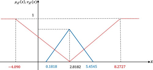
Hence:
and the total IF cost is determined as follows (Figure ):
Example 5.2:
In the paper [Citation16], we suppose that the objective function coefficients and the technology coefficients are crisp. Then
where,
and
Solving this problem by our method, we would have:
and
Using the method applied in [Citation16], the results would be:
and
in comparison, based on the achieve results, it is obvious that our method is better.
Figure 2. Graphical representation of IF optimal costs.
Example 5.3:
In Example 5.2, we just consider the fuzzy part of the numbers and solve it with the ranking function used in [Citation47]. Then and
Obviously, a better answer will be obtained when the numbers are considered intuitionistic fuzzy.
Example 5.4:
Ekbatan oil refinery is able to extract three types of crude oil from its oil wells in three different cities. These three types of crude oil must be combined with two other types of additives to obtain gasoline. Table shows the amount of sulphur and other additives, including lead and phosphorus used in crude oil.
Table 3. Information on crude oil and its additives.
The amount of sulphur in each gallon of gasoline should be a maximum of about 0.07 per cent.
The amount of lead in each gallon of gasoline should be about between 1.25 and 2.5 grams.
The amount of phosphorus in each gallon of gasoline should be about between 0.0025–0.0045 grams.
The total amount of additives should not be more than about 0.19 percentage of the composition of gasoline produced.
The question is, what combination of crude oil should we consider in order to minimise the cost of producing gasoline?
Solve:
Because of uncertainty in resources, the problem can be modeled as an IFVLP problem by using TIFNs. So we will have
where,
Remark 5.1:
We emphasis that the above numerical discussion is given to explain our suggested theoretical results as well as the extension of the duality theorems and results in fuzzy environment. We saw that some of these numerical examples are compared with the other works which was used some ranking functions.
6. Conclusion
In this paper, we formulated a kind of linear programming problems involving intuitionistic fuzzy variables. We investigated the dual of this problem with intuitionistic fuzzy parameters. Also, we developed some duality results, including weak and strong duality and also complementary slackness, for the intuitionistic fuzzy problems. Using these results, we proposed a solution approach and a dual simplex algorithm for the IFVLP problem. The approach offered here is useful for sensitivity analysis. However, considering post analysis results in IFLP problems is a worthwhile area of research that will be investigated in our future works.
Acknowledgments
The authors would like to appreciate from the anonymous referees who help us to improve the earlier versions of this manuscript based on their constructive comments and the valuable suggestions.
Disclosure statement
No potential conflict of interest was reported by the author(s).
Additional information
Notes on contributors
M. Goli
M. Goli received his B.S. degree in Applied Mathematics, Faculty of Mathematical Sciences, Shahrood University of Technology (2009-2013). He obtained his M.Sc. degree in Applied Mathematics, Operations Research, Faculty of Mathematical Sciences, Shahrood University of Technology (2013-2015). Now. He is a Ph.D student in Applied Mathematics, Operations Research, Faculty of Mathematical Sciences, University of Mazandaran, Babolsar, Iran.
S. H. Nasseri
S. H. Nasseri received his Ph.D degree in 2007 on Fuzzy Mathematical Programming from Sharif University of Technology, and since 2007 he has been a faculty member at the Faculty of Mathematical Sciences in University of Mazandaran, Babolsar, Iran. During this program, he also got JASSO Research Scholarship from Japan (Department of Industrial Engineering and Management, Tokyo Institute and Technology (TIT), Tokyo, 2006–2007). Recently, in 2018, he also completed a postdoctoral program at the Department of Industrial Engineering, Sultan Qaboos University, Muscat, Oman on Logistic on Uncertainty Conditions. Also, he collaborated with Foshan University (Department of Mathematics and Big Data), Foshan, China as a visiting professor, since 2018. He serves as the Editor-in-Chief (Middle East Area) of Journal of Fuzzy Information and Engineering since 2014 and the Editorial board member of five reputable academic journals. He is a council member of the International Association of Fuzzy Information and Engineering, a Standing Director of the International Association of Grey Systems and Uncertainty Analysis since 2016, and vice-president of Iranian Operations Research Society. International Center of Optimization and Decision Making is established by him in 2014. His research interests are in the areas of Fuzzy Mathematical Models and Methods, Fuzzy Arithmetic, Fuzzy Optimization and Decision Making, Operations Research, Gray Systems, Logistics and Transportation.
References
- Zadeh LA. Fuzzy sets. Inf Control. 1965;8:338–353.
- Tanaka H, Okuda T, Asai K. On fuzzy mathematical programming. J Cybern Syst. 1973;3:37–46.
- Bellman RE, Zadeh LA. Decision making in a fuzzy environment. Manage Sci. 1970;17:B-141–B-164.
- Noori-Skandari MH, Ghaznavi M. An efficient algorithm for solving fuzzy linear programming problems. Neural Processing Letters. 2018;48:1563–1582.
- Zimmermann HJ. Fuzzy programming and linear programming with several objective functions. Fuzzy Sets Syst. 1978;1:45–55.
- Nasseri SH, Ebrahimnejad A. A new approach to duality in fuzzy linear programming. Fuzzy Eng Oper Res. 2010;147:17–29.
- Ghaznavi M, Soleimani F, Hoseinpoor N. Parametric analysis in fuzzy number linear programming problems. Int J Fuzzy Syst. 2016;18:463–477.
- Mahdavi-Amiri N, Nasseri SH, Yazdani A. Fuzzy primal simplex method for solving fuzzy linear programming problems. Iran J Oper Res. 2009;1:68–84.
- Campos L, Verdegay JL. Linear programming problems and ranking of fuzzy numbers. Fuzzy Sets Syst. 1989;32:1–11.
- Mahdavi-Amiri N, Nasseri SH. Duality in fuzzy number linear programming by use of a certain linear ranking function. Appl Math Comput. 2006;180:206–216.
- Ebrahimnejad A, Nasseri SH, Mansourzadeh SM. Modified bounded dual network simplex algorithm for solving minimum cost flow problem with fuzzy costs based on ranking functions. J Intell Fuzzy Syst. 2013;24:191–198.
- Muralidaranand C, Venkateswarlu B. Generalized ranking function for all symmetric fuzzy linear programming problems. J Intell Fuzzy Syst. 2018;20:1–5.
- Roldan L AF, Hierro D, Roldan C, et al. On a new methodology for ranking fuzzy numbers and its application to real economic data. Fuzzy Sets Syst. 2018;21:1–25.
- Xuan Chi HT, Yu VF. Ranking generalized fuzzy numbers based on centroid and rank index. Appl Soft Comput. 2018;18:1–36.
- Atanassov KT. Intuitionistic fuzzy sets. Fuzzy Sets Syst. 1986;20:87–96.
- Nagoorgani A, Ponnalagu K. A method based on intuitionistic fuzzy linear programming for investment strategy. Int J Fuzzy Math Arch. 2016;10:71–81.
- Seikh MR, Nayakand PK, Pal M. Notes on triangular intuitionistic fuzzy numbers. Int J Math Operational Res. 2013;5:446–465.
- Atalik G, Senturk S. A new lexicographic ranking method for triangular intuitionistic fuzzy number based on gergonne point. J Quant Sci. 2019;1:59–73.
- Suresh M, Vengataasalam S, ArunPrakash K. Solving intuitionistic fuzzy linear programming problems by ranking function. J Intell Fuzzy Syst. 2014;27:3081–3087.
- Darehmiraki M. A novel parametric ranking method for intuitionistic fuzzy numbers. Iran J Fuzzy Syst. 2019;16:129–143.
- Das D, De PK. Ranking of intuitionistic fuzzy numbers by new distance measure. J Intell Fuzzy Syst. 2016;30:1099–1107.
- Nayagam VLG, Jeevaraj S, Geetha S. Total ordering for intuitionistic fuzzy numbers. Complexity. 2016;21:54–66.
- Mitchell HB. Ranking intuitionistic fuzzy numbers. Int J Uncertainity Fuzziness Knowledge Based Syst. 2004;12:377–386.
- Sidhu SK, Kumar A. A note on solving intuitionistic fuzzy linear programming problems by ranking function. J Intell Fuzzy Syst. 2016;30:2787–2790.
- Uthra G, Thangavelu K, Shunmugapriya S. Ranking generalized intuitionistic pentagonal fuzzy number by centroidal approach. Int J Math App. 2017;5:589–593.
- Angelov P. Optimization in an intuitionistic fuzzy environment. Fuzzy Sets Syst. 1997;86:299–306.
- Cherian L, Kuriakose AS. Intuitionistic fuzzy optimization for linear programming problems. J Fuzzy Math. 2012;17:139–144.
- Parvathi R, Malathi C. Arithmetic operations on symmetric trapezoidal intuitionistic fuzzy numbers. Int J Soft Comput Eng (IJSCE). 2012;2:268–273.
- Parvathi R, Malathi C. Intuitionistic fuzzy linear programming problems. World Appl Sci J. 2012;17:1802–1807.
- Ejegwa PA, Akowe SO, Otene PM, et al. An overview on intuitionistic fuzzy sets. Int J Sci Technol Res. 2014;3:142–145.
- Dubey D, Mehra A. Linear programming with triangular intuitionistic fuzzy numbers. Adv Intell Syst Res. 2011;1:563–569.
- Nagoorgani A, Ponnalagu K. An approach to solve intuitionistic fuzzy linear programming problem using single step algorithm. Int J Pure Appl Math. 2013;86:819–832.
- Nasseri SH, Goli M. On solving fully intuitionistic fuzzy linear programming problem). The 11th International conference of Iranian operations research society; 2018. p. 140–144.
- Nagoorgani A, Ponnalagu K. Solving linear programming problem in an intuitionistic environment. Proc Heber Int Conf Appl Math Stat HICAMS. 2012;3:29–46.
- Nachammai AL, Thangaraj P. Solving intuitionistic fuzzy linear programming problem by using similarity measures. Eur J Sci Res. 2012;72:204–210.
- Hepzibah RI, Vidhya R. Modified new operations for symmetric trapezoidal intuitionistic fuzzy numbers: An application of diet problem. Int J Fuzzy Math Arch. 2015;9:35–43.
- Sidhu SK. A new approach to solve intuitionistic fuzzy linear programming problems with symmetric trapezoidal intuitionistic fuzzy numbers. Math Theory Model. 2015;5:66–74.
- Nasseri SH, Goli M, Bavandi S. An approach for solving linear programming problem with intuitionistic fuzzy objective coefficient). The 6th Iranian joint congress on fuzzy and intelligent systems; 2018. p. 104–107.
- Prabakaran K, Ganesan K. Duality theory for intuitionistic fuzzy linear programming problems. Int J Civ Eng Technol (IJCIET). 2017;8:546–560.
- Sidhu SK, Kumar A. Mehar methods to solve intuitionistic fuzzy linear programming problems with trapezoidal intuitionistic fuzzy numbers. Perform Predict Anal Fuzzy Reliab Queuing Model Asset Anal. 2019;21:265–282.
- Ramík J, Vlach M. Intuitionistic fuzzy linear programming and duality: a level sets approach. Fuzzy Optim Decis Mak. 2016;15:457–489.
- Ban A. Intuitionistic fuzzy measures. New York: Nova Science Publisheds; 2006.
- Burillo P, Bustince H, Mohedano V, et al. Some definitions of intuitionistic fuzzy number. First Prop Proc First Workshop Fuzzy Based Expert Syst. 1994;5:53–55.
- Grzegorzewski P. Distances and orderings in a family of intuitionistic fuzzy numbers. Proc. of the third conf. of the European Society for fuzzy logic and technology EUSFLAT, 1; 2003. p. 223–227.
- Kabiraj A, Nayak PK, Raha SW. Solving intuitionistic fuzzy linear programming problem. Int J Intell Sci. 2019;9:44–58.
- Nasseri SH, Ebrahimnejad A, Cao BY. Fuzzy linear programming: solution techniques and applications. Switzerland: Springer; 2019.
- Mahdavi-Amiri N, Nasseri SH. Duality results and a dual simplex method for linear programming problems with trapezoidal fuzzy variables. Fuzzy Sets Syst. 2007;158:1961–1978.