A Profit Maximisation Solid Transportation Problem Using Genetic Algorithm in Fuzzy Environment

Abstract

In this paper, a solid transportation problem has been considered in which the transportation is accomplished in two stages – firstly, from the origin(s) to the near by station(s) of the destination(s) and secondly, from the near by station(s) to the exact destination(s). Here, a fuzzy AUD (all unit discount) policy has been introduced based upon the amount of transportation along with a fuzzy fixed charge. In addition, a budget constraint has been incorporated taking fuzzy unit transportation cost. Then the proposed model has been converted into a single objective optimisation problem using interval arithmetic method. To solve the model, Genetic Algorithm (GA) has been used depending on roulette wheel selection, crossover and mutation. Finally, a numerical example has been illustrated to study the feasibility of the model.

KEYWORDS:

• All unit discount
• genetic algorithm
• profit maximisation solid transportation problem
• fuzzy resource and demand

1. Introduction

In reality, the decision making problem [1–3] become an important criteria in our daily life. Transportation problem (TP) is one of such important decision making problem. Hitchcock [4] first defined the transportation problems (TP) as one of the most common special type linear programming problems involving constraints. The traditional TP is a well-known optimisation problem in operational research, in which two kinds of constraints are taken into consideration. But in the real system, we always deal with other constraint besides of source constraint and destination constrain, such as transportation mode constraint. For such case, the traditional TP turns into the solid transportation problem (STP) which was stated by Shell [5]. He suggested the situation where the solid transportation problem would arise. The STP is a generalisation of traditional transportation problem. Recently, Samanta et al. [6] solved a fuzzy STP following two level fuzzy programming technique. Pan et al. [7] discuss different fuzzy programming technique to solve different decision making problem. The necessity of considering this special type of transportation problem arises when heterogeneous conveyances are available for shipment of products. The STP is arisen in public distribution systems. A homogeneous product is delivered from an origin to a destination by means of different modes of transport called conveyances, such as trucks, goods trains and ships. These conveyances are taken as the third dimension. A solid transportation problem can be converted to a classical transportation problem by considering only a single type of conveyance.

In many practical applications, it is realistic to assume that the amount which can be sent on any particular route bears an uncertain fixed charge for that route. Further, when a route is altogether excluded, this can be expressed by limiting its capacity to zero. Such fixed transportation costs may also be applied to some production-planning models. Ojha et al. [8] consider such type of fixed charge as well as vehicle cost in STP in deterministic forms. There are also another existing literature in which the fixed charge has been considered in deterministic nature. Till now, no one has considered fixed charge and vehicle cost together in imprecise nature. Recently, Dalman et al. [9] proposed a Multi-objective Multi-item Solid Transportation Problem Under Uncertainty.

Jimecncz and Verdegay [10] solved both interval and fuzzy solid transportation problem by an extension of auxiliary linear programme proposed by Chanas et al. [11]. Intuitively, when the cost coefficients or the supply and demand quantities are fuzzy numbers, the total transportation will be fuzzy as well. Li et al. [12] utilised improved genetic algorithm to solve the fuzzy multi-objective solid transportation problems, where the cost coefficients objective function are fuzzy numbers. Bit et al. [13] Jimenez and Verdegay [14], Das et al. [15], Li and Lai [12] and Waiel [16] presented the fuzzy compromise programming approach to multi-objective transportation problems. Grzegorzewski [17] approximated the fuzzy number to its nearest interval. Omar and Samir [18] and Chanas and Kuchta [11] discussed the solution algorithm for solving the transportation problem in fuzzy environment. Very recently, Ojha et al. [8,19] presented the STP in different type of uncertain environment. Huang [20] discuss the Signed distance and Centroid method to defuzzify the fuzzy parameters.

In this paper, a fuzzy solid transportation problem is considered as profit maximisation problem following Sakawa et al. [21]. Generally TP is a minimising problem. In that case how much cost will be occurred to delivered the item from different origin to the different destination i.e. suppose different retailer how much total cost will be occurred i.e. calculated as minimised problem. But new thing is that in this case we consider maximisation, in the respect that the destination centre there are some retailer. Getting the item, and retailers are cell the item to the customer. In that respect we consider the how much profit will be occurred after selling these item which is transported. The path from source(s) to destination(s) is divided into two parts on the basis of the permit of road capacity of the convenance. Here, a discount is given to the unit cost of transportation which depends on the amount of transportation, AUD cost is also imprecise in nature. All traditional constraints are also fuzzy. In addition, a budget constraint is taken on the transportation cost. There are several non-analytic processes to find the solution of a linear/non-linear programming problem such as neural network [22], analytic hierarchy process [23], etc. The proposed model has been optimised using Genetic Algorithm (GA) (cf. Goldberg [24], Ju et al. [25], Basu et al. [26], Maiti and Maiti [27]). Finally, a numerical example is illustrated. The basic differences of the proposed model from other existing models in this chapter have been given in Table 1.

Table 1. Comparison table among the existing models with proposed model.

References(s)	Unit Trans. Cost	Fixed Charge	Vehicle Cost	Profit	Solving Method
Bit et al. [13]	Fuzzy	No	No	No	Fuzzy programming
Sakawa et al. [21]	Fuzzy	No	No	Yes	Fuzzy programming
Liu et al. [29]	Fuzzy	Yes, Crisp	No	No	GA
Ojha et al.	Crisp AUD	Yes, Crisp	Yes	No	GA
Li et al. [12]	Fuzzy	No	No	No	GA
This model	Fuzzy AUD	Yes, Fuzzy	Yes with two different capacities	Yes	GA

Now I see what is the new thing in this model. So we see the basic different is the profit model with other existing model. In this model one novibility is that transportation cost. Here we consider fuzzy AUD transportation cost. Those AUD cost has been consider earlier by ojha. But in that case that was scrip, but here we consider fuzzy AUD TP cost. Other thing is that fixed charge, here we consider fuzzy fixed charge though earlier researcher not consider fuzzy fixed charge. The vehicle cost to transport the item from source to destination, there is several type vehicle cost, here we consider two type of vehicle cost depending on the basis of capacity. And last thing is profit maximisation. That is the new thing i.e. it consider respect to retailer.

2. Preliminaries

2.1. Fuzzy Set

The fuzzy set theory was developed to define and solve the complex system with sources of uncertainty or imprecision which are non-statistical in nature. Fuzzy set theory is a theory of graded concept (a matter of degree) but not a theory of chance or probability.

A fuzzy set is a class of objects in which there is no sharp boundary between those objects that belong to the class and those that do not. Let X be a collection of objects and x be an element of X, then a fuzzy set $\tilde{A}$ in X is a set of ordered pairs $\tilde{A}=\{(x,{\mu }_{\tilde{A}}(x))/x\in X\}$

where ${\mu }_{\tilde{A}}(x)$ is called the membership function or grade of membership of x in $\tilde{A}$ which maps X to the membership space M which is considered as the closed interval [0,1].

Equality: Two fuzzy sets $\tilde{A},\tilde{B}$ are said to be equal if and only if ${\mu }_{\tilde{A}}(x)={\mu }_{\tilde{B}}(x),\mathrm{\forall }x\in X.$

Containment: A fuzzy set $\tilde{A}$ is contained in or is a subset of a fuzzy set $\tilde{B}$, written as $\tilde{A}\subset \tilde{B}$ if and only if ${\mu }_{\tilde{A}}(x)\le {\mu }_{\tilde{B}}(x),\mathrm{\forall }x\in X.$

Narmality: A fuzzy set $\tilde{A}$ is normal if there exist at least one element $x\in F$ such that ${\mu }_{\tilde{A}}(x)=1$.

Convexity: Let $\tilde{A}$ fuzzy set in X. Then $\tilde{A}$ is convex if and only if for any $x_1,x_2\in X,$ the membership function of $\tilde{A}$ satisfies the inequality ${\mu }_{\tilde{A}}(w_1{x}_1+(1-w_1)x_2)\ge min({\mu }_{\tilde{A}}(x_1),{\mu }_{\tilde{A}}(x_2))$ for $0\le w_1\le 1.$

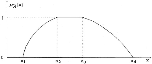
Fuzzy Number: A fuzzy number is a special class of a fuzzy sets. A fuzzy subset $\tilde{A}$ of real number R with membership function ${\mu }_{\tilde{A}}:R\to [0,1]$ is called a fuzzy number if it satisfies the following

• $\tilde{A}$ is normal.

• $\tilde{A}$ is convex.

• $\tilde{A}$ upper semi-continuous and

• Supp($\tilde{A}$) is bounded here $Supp(\tilde{A})=cl\{x\in R:{\mu }_A(x)>0\}$ and cl is the closer operator. The membership function of General fuzzy number à represented by Figure 1.

Figure 1. Membership function of General fuzzy number $\tilde{A}$_.

Some standard fuzzy numbers are discussed in the following

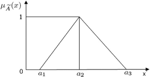
Triangular Fuzzy Number (TFN): A triangular fuzzy number $\tilde{A}$, with continuous membership function ${\mu }_{\tilde{A}}(x):X\to [0,1]$ which can be specified by the triplet $(a_1,a_2,a_3)$ is as follows: ${\mu }_{\tilde{A}}(x)=\{\begin{array}{ll}0& ifx\le a_1\\ {\displaystyle \frac{x-a_1}{a_2-a_1}}& if{a}_1\le x\le a_2\\ {\displaystyle \frac{a_3-x}{a_3-a_2}}& if{a}_2\le x\le a_3\\ 0& ifx\ge a_3\end{array}$

And membership function of TFN Ã graphically is Figure 2.

Figure 2. Membership function of TFN $\tilde{A}$_.

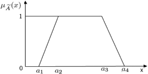
Trapezoidal Fuzzy Number (TrFN): TrFN is the fuzzy number with the membership function ${\mu }_{\tilde{A}}(x)$, a continuous mapping ${\mu }_{\tilde{A}}(x):R\to [0,1]$ ${\mu }_{\tilde{A}}(x)=\{\begin{array}{ll}{\displaystyle \frac{x-a_1}{a_2-a_1}}& for{a}_1\le x\le a_2\\ 1& for{a}_2\le x\le a_3\\ {\displaystyle \frac{a_4-x}{a_4-a_3}}& for{a}_3\le x\le a_4\\ 0& otherwise\end{array}$

And membership function of TrFN Ã graphically is Figure  3.

Figure 3. Membership function of TrFN $\tilde{A}$

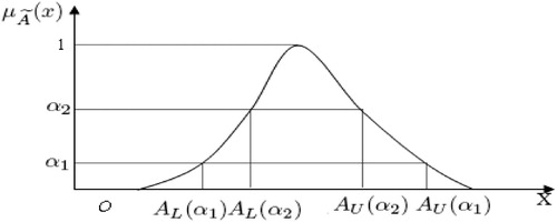
$\mathit{\alpha }$-Cut of a fuzzy number: An $\alpha$- cut of a fuzzy number $\tilde{A}$ is defined as crisp set $A_{\alpha }=\{x:{\mu }_{\tilde{A}}(x)\ge \alpha ,x\in X\}where\alpha \in [0,1]$ $A_{\alpha }$ is a non-empty bounded closed interval contained in $X$ and it can be denoted by $A_{\alpha }=[A_L(\alpha ),A_U(\alpha )]$. $A_L(\alpha )$ and $A_U(\alpha )$ are the lower and upper bounds of the closed interval respectively. A fuzzy number $\tilde{A}$ with ${\alpha }_1,{\alpha }_2$ - cut $A_{{\alpha }_1}=[A_L({\alpha }_1),A_U({\alpha }_1)],A_{{\alpha }_2}=[A_L({\alpha }_2),A_U({\alpha }_2)]$ and if ${\alpha }_2\ge {\alpha }_1$, then $A_L({\alpha }_2)\ge A_L({\alpha }_1)$ and $A_U({\alpha }_1)\ge A_U({\alpha }_2)$. The α- cut of a fuzzy number à represented by Figure  4.

Figure 4. $\alpha$- cut of a fuzzy number $\tilde{A}$_.

2.2. Interval Analysis

An interval valued number is a closed interval defined by $A=[a_L,a_U]=\{x:a_L\le x\le a_U,x\in R\}$ where $a_L$ and $a_U$ are the left and right limits respectively and R denotes for the set of all real numbers. It is also defined by its centre and radius as $A=(a_c,a_r)=\{x:a_c-a_r\le x\le a_c+a_r,x\in R\}$ where the centre and radius are denoted by $a_c=(a_L+a_U)/2$ and $a_r=(a_U-a_L)/2$

Particularly, each real number can be regarded as an interval, such as, for all $x\in R$, $x$ can be written as an interval $[x,x]$, which has zero width. Now, we shall give the concise definitions of first four arithmetical operations of intervals.

Definition 2.2.1.

Let $\ast$ be a binary operation on the set of real numbers. If $A$ and $B$ are two closed intervals then $A\ast B=\{a\ast b:a\in Aandb\in B\}$ defines a binary operation on the set of closed intervals. In the case of division, it is assumed that 0  B.

For two interval numbers $A=[a_L,a_U]$ and $B=[b_L,b_U]$, the operations on interval may be explicitly calculated from definition 1 as $A+B=[a_L+a_U,b_L+b_U],$ $A-B=[a_L-b_U,a_U-b_L],$ $\lambda A=\{\begin{array}{l}[\lambda a_L,\lambda a_U]if\lambda \ge 0,\\ [\lambda a_U,\lambda a_L]if\lambda \le 0\end{array}$ where $\lambda$ is a real number.

Definition 2.2.2.

For minimising problem, let us define the order relation ${\le }_p$ between $A=[a_L,a_U]=⟨a_c,a_r⟩$ and $B=[b_L,b_U]=⟨b_c,b_r⟩$ as $A{\le }_{p}B\iff a_c\le b_c,$ $A{<}_{p}B\iff A{\le }_{p}B\wedge A\ne B.$

Definition 2.2.3.

Using Definition 2, we can easily define the order relation ${\ge }_p$ between $A=[a_L,a_U]=⟨a_c,a_r⟩$ and $B=[b_L,b_U]=⟨b_c,b_r⟩$ for Maximising problem as $A{\ge }_{p}B\iff a_c\ge b_c,$ $A{>}_{p}B\iff A{\ge }_{p}B\wedge A\ne B.$

3. Notations and Assumptions of the Proposed Model

3.1. Notations

In this solid transportation problem, the following notations have been used

• $M$ = no of sources of the transportation problem.

• $N$ = no of demands of the transportation problem.

• $K$ = no of conveyances i.e. different modes of the transportation problem.

• $O_i,{\tilde{O}}_i$ = crisp and fuzzy origins of the transportation problem.

• $D_j,{\tilde{D}}_j$ = crisp and fuzzy destination of the transportation problem.

• $E_k,{\tilde{E}}_k$ = crisp and fuzzy conveyances of the transportation problem.

• $a_i,{\tilde{a}}_i$ = crisp and fuzzy amount of a homogeneous product available at i-th origin.

• $b_j,{\tilde{b}}_j$ = crisp and fuzzy demand at j-th destination.

• $e_k,{\tilde{e}}_k$ = crisp and fuzzy amount of product which can be carried by k-th conveyance.

• $f_{ijk},{\tilde{f}}_{ijk}$ = crisp and fuzzy fixed charge of the transportation problem.

• $C_{ijk},{\tilde{C}}_{ijk}$ = crisp and fuzzy unit transportation cost.

• $V_{ijk}$ = transportation vehicle cost per unit item.

• $x_{ijk}$ = amount of the product to be transported from i-th supply to j-th demand node by k-th conveyance.

• $S_i$ = unit selling price.

• $D$ = total maximum direct cost.

3.2. Assumptions

To develop the proposed solid transportation model, the following assumptions have been made.

• In the traditional transportational problem, it is seen that the quantity is transported from a source to a destination by one convenance only. But, in practical business system, it is not always true. There exist some transportation problems in which the materials required can not be transported directly from the source to the destination by one convenance only. In such situation the materials are transported to a station near by the destination by one convenance only and then from this near by station, it is transported to the exact destination by another convenance.

• For transportation the material from the near by station to the exact destination, a vehicle cost,$V$ has been assumed. Here, two types of vehicles such as one having large loading capacity to be $G_c$ and another having small loading capacity to be $G_c^{{}^{\mathrm{\prime }}}$ i.e. $G_c>G_c^{{}^{\mathrm{\prime }}}$ have been considered and the corresponding vehicle cost for large and small vehicles are $G$ and $G^{\mathrm{\prime }}$ respectively. Therefore, the total vehicle cost $V(x_{ijk})$ to be transported the items of amount $x_{ijk}$ has been proposed in the following form (1) $V(x_{ijk})=\{\begin{array}{l}h.Gifh.G_c=x_{ijk}\\ h.G+G^{\mathrm{\prime }}if{x}_{ijk}-h.G_c>0\end{array}$(1) where $h=[x_{ijk}/G_c]$ and $[x]$ denotes the greatest integer but less then equal to $x$.

• For transportation the materials from i-th source to the near by place of j-th destination by k-th convenance, the unit transportation cost $Cijk$ have been discounted on the basis of transported amount according to AUD policy. Again, it is seen that due to the various factors the unit transportation costs may also vary i.e. realistically it may be uncertain. In this paper, it has been considered as fuzzy numbers. Therefore, the fuzzy unit transformation costs ${\tilde{C}}_{ijk}$ have been taken in the following form (2) ${\tilde{C}}_{ijk}=\{\begin{array}{l}{\tilde{c}}_{1ijk}if0<x_{ijk}<R_1\\ {\tilde{c}}_{2ijk}if{R}_1\le x_{ijk}<R_2\\ \dots \dots \dots \dots ..\\ \dots \dots \dots \dots ..\\ {\tilde{c}}_{tijk}if{R}_{(t-1)}\le x_{ijk}<R_t\\ {\tilde{c}}_{(t+1)ijk}if{R}_t\le x_{ijk}\end{array}$(2) $here{\tilde{c}}_{1ijk}>{\tilde{c}}_{2ijk}>{\tilde{c}}_{3ijk}>\dots ..>{\tilde{c}}_{tijk}>{\tilde{c}}_{(t+1)ijk}areallunitcost.$

• A fixed charge was taken into consideration at the time transportation like, road taxes, etc. Assume that a homogeneous product is to be transported from $M$ sources to $N$ destinations by $K$ different transport modes. Furthermore, a fixed charge ${\tilde{f}}_{ijk}$, is related to the transportation that a unit of this product is carried with $k-th$ transport mode from the source $i-th$ to the destination $j-th$. Assume that $y$ is function of $x_{ijk}$ takes the values $0$ and $1$ to describe the transportation activity from source $i-th$ to destination $j-th$ through transport mode $k-th$ and is defined as (3) $y(x_{ijk})=\{\begin{array}{l}1,if0<x_{ijk}\\ 0,otherwise\end{array}$(3)

Also fixed charge ${\tilde{f}}_{ijk}$ are taken as fuzzy then the the total fixed charge ${\tilde{d}}_{ijk}$ is in the form: ${\tilde{d}}_{ijk}={\tilde{f}}_{ijk}y(x_{ijk})$

• Direct costs (such as for labour, material, fuel or power) vary with the rate of output but are uniform for each unit of production and are usually under the control and responsibility of the department manager. As a general rule, most costs are fixed in the short run and variable in the long run. So, we considered a boundedness of direct transportation cost.

• In traditional transportation problem, we determined the minimum transportation cost. Here, we assume thatthe items are selling at destination. In that case profit will considered. Profit is taken into account. And profit is maxmised which ia equivalant to the maxmisation oh total transportation cost.

4. Mathematical Formulation of a Solid Transportation Problem

In this model, we consider a homogeneous product to be transported from each $M$ sources [$O_i$, $i=1,2,\dots .M$] to $N$ destinations [$D_j$, $j=1,2,\dots .N$] via $K$ conveyances [$E_k$, $k=1,2,\dots .K$]. The available capacities of sources like warehouses, production facilities or supply quantities are ${\tilde{a}}_i$,($i=1,2,\dots .M$). The destination are consumption facilities, warehouses, or demand points, characterised by required levels of demand ${\tilde{b}}_j$ ($j=1,2,\dots .N$) and ${\tilde{e}}_k$ ($k=1,2,\dots .K$) represents the amount of product which can be carried by k-th conveyance. ${\tilde{C}}_{ijk}$ be the unit cost under AUD systems associated with transportation of a unit product from i-th source to j-th destination by means of the k-th conveyance which is imprecise in nature. we consider the unit purchasing price for each item at i-th source be ${\tilde{R}}_i$ ($i=1,2,\dots .M$) Also we consider the unit selling price for each item at j-th destination be ${\tilde{S}}_j$ ($j=1,2,\dots .N$)then the problem is converted into a profit maximisation problem subject to traditional transportation constraints and boundedness of direct transportation cost. (4) $\begin{array}{rl}Max\tilde{P}(x_{ijk})& =\sum _{j=1}^N\left\{{\tilde{S}}_j\sum _{i=1}^M\sum _{k=1}^K{x}_{ijk}\right\}-\{\sum _{i=1}^M\left({\tilde{R}}_i\sum _{j=1}^N\sum _{k=1}^K{x}_{ijk}\right)+\sum _{i=1}^M\sum _{j=1}^N\sum _{k=1}^K{\tilde{C}}_{ijk}{x}_{ijk}\\ & +\sum _{i=1}^M\sum _{j=1}^N\sum _{k=1}^K{\tilde{d}}_{ijk}+\sum _{i=1}^M\sum _{j=1}^N\sum _{k=1}^{K}V(x_{ijk})\}\end{array}$(4) subject to (5) $\sum _{j=1}^N\sum _{k=1}^K{x}_{ijk}={\tilde{a}}_{i}i=1,2,3,\dots ,M$(5) (6) $\sum _{i=1}^M\sum _{k=1}^K{x}_{ijk}={\tilde{b}}_{j}j=1,2,3,\dots ,N$(6) (7) $\sum _{i=1}^M\sum _{j=1}^N{x}_{ijk}={\tilde{e}}_{k}k=1,2,3,\dots ,K$(7) (8) $\sum _{i=1}^M\sum _{j=1}^N\sum _{k=1}^K{\tilde{C}}_{ijk}{x}_{ijk}\le \tilde{D}$(8) where ${\tilde{C}}_{ijk}$ are given by (2) for AUD.

4.1. Defuzzification of the Model

In the model with Equations 6–10, ${\tilde{a}}_i,{\tilde{b}}_j,{\tilde{e}}_k,{\tilde{C}}_{ijk},{\tilde{d}}_{ijk}$ and ${\tilde{S}}_i$ have been taken as fuzzy numbers with $\alpha$-cuts are $[a_{iL},a_{iU}]$,$[b_{jL},b_{jU}]$,$[e_{kL},e_{kU}]$,$[C_{ijkL},C_{ijkU}]$, $[d_{ijkL},d_{ijkU}]$, and $[S_{iL},S_{iU}]$ respectively. Let $\tilde{A}=(a_1,a_2,a_3)$ be a triangular fuzzy number then left and right cut of $\tilde{A}$ are $A_L(\alpha )=a_1+\alpha (a_2-a_1)$ and $A_U(\alpha )=a_3-\alpha (a_3-a_2)$. Also let $\tilde{B}=(b_1,b_2,b_3,b_4)$ be a trapezoidal fuzzy number then left and right cut of $\tilde{B}$ are $B_L(\alpha )=b_1+\alpha (b_2-b_1)$ and $B_U(\alpha )=b_4-\alpha (b_4-b_3)$.

Therefore using interval arithmetic $\alpha$-cut of the profit is given by (9) $\tilde{P}(x_{ijk},\alpha )=[P_L(x_{ijk},\alpha ),P_U(x_{ijk},\alpha )]$(9) where $\begin{array}{rl}{P}_L(x_{ijk},\alpha )& =\sum _{j=1}^N\left\{S_{jL}\sum _{i=1}^M\sum _{k=1}^K{x}_{ijk}\right\}-\sum _{i=1}^M\left\{R_{iU}\sum _{j=1}^N\sum _{k=1}^K{x}_{ijk}\right\}-\sum _{i=1}^M\sum _{j=1}^N\sum _{k=1}^K{C}_{ijkU}{x}_{ijk}\\ & -\sum _{i=1}^M\sum _{j=1}^N\sum _{k=1}^K{d}_{ijkU}-\sum _{i=1}^M\sum _{j=1}^N\sum _{k=1}^{K}V(x_{ijk}),\end{array}$ and $\begin{array}{rl}{P}_U(x_{ijk},\alpha )& =\sum _{j=1}^N\left\{S_{jU}\sum _{i=1}^M\sum _{k=1}^K{x}_{ijk}\right\}-\sum _{i=1}^M\left\{R_{iL}\sum _{j=1}^N\sum _{k=1}^K{x}_{ijk}\right\}-\sum _{i=1}^M\sum _{j=1}^N\sum _{k=1}^K{C}_{ijkL}{x}_{ijk}\\ & -\sum _{i=1}^M\sum _{j=1}^N\sum _{k=1}^K{d}_{ijkL}-\sum _{i=1}^M\sum _{j=1}^N\sum _{k=1}^{K}V(x_{ijk})\end{array}$ subject to (10) $\sum _{j=1}^N\sum _{k=1}^K{x}_{ijk}\in [a_{iL},a_{iU}]\text{ equivalent to }{a}_{iL}\le \sum _{j=1}^N\sum _{k=1}^K{x}_{ijk}\le a_{iU}$(10) (11) $\sum _{i=1}^M\sum _{k=1}^K{x}_{ijk}\in [b_{jL},b_{jU}]\text{equivalent to}{b}_{jL}\le \sum _{i=1}^M\sum _{k=1}^K{x}_{ijk}\le b_{jU}$(11) (12) $\sum _{i=1}^M\sum _{j=1}^N{x}_{ijk}\in [e_{kL},e_{kU}]\text{ equivalent to}{e}_{kL}\le \sum _{i=1}^M\sum _{j=1}^N{x}_{ijk}\le e_{kU}$(12) (13) $D_L\le \sum _{i=1}^M\sum _{j=1}^N\sum _{k=1}^K\left[\frac{C_{ijkL}+C_{ijkU}}{2}\right]x_{ijk}\le D_U$(13)

So, the problem reduces to determine $x_{ijk}$ so that $\tilde{P}(x_{ijk},\alpha )$ is maximum for fixed $\alpha$ subject to the constrain (11)–(14).

5. Solution Procedures

To find the optimal solution of above constraint solid transportation problem, we use the C-language GA. Genetic Algorithm for the Linear and Nonlinear Transportation Problem was developed by G.A. Vignauz and Z. Michalewic [28]. As the name suggests, GA is originated from the analogy of biological evolution. GAs consider a population of individuals. Using the terminology of genetics, a population is a set of feasible solutions of a problem. A member of the population is called a genotype, a chromosome, a string or a permutation. The advantages of GA are

1. Optimise the objective functions with continuous or discrite decision variables

2. do not require the derivative information of the objective function

3. Easy to exploit previous or alternate solutions

4. deal with a large number of decision variables

5. work with numerically generated data, experimental data or analytical functions.

Procedures for different GA components

5.1. Chromosome Representation

The concept of chromosome is normally used in the GA to stand for a feasible solution to the problem. A chromosome has the form of a string of genes that can take on some value from a specified search space. Normally, there are two types of chromosome representation – (i) the binary vector representation and (ii) the real number representation. Here, the real number representation scheme is used. A ‘K dimensional real vector’ X = (x${}_1$, x${}_2$, … . x${}_K$) is used to represent a solution, where x${}_1$, x${}_2$, … . x${}_K$ represent different decision variables of the problem. In the proposed model, $k=8$. Here, $x_1,x_2,x_3,x_4,x_5,x_6,x_7$ and $x_8$ denote the variables $x_{111},x_{121},x_{112},x_{122},x_{211},x_{221},x_{212}$ and $x_{222}$ respectively.

5.2. Initialisation

A set of solutions (chromosomes) is called a population. N such solutions X${}_1$, X${}_2$, X${}_3$, … X${}_N$ are randomly generated from search space by random number generator such that each X${}_i$ satisfies the constraints of the problem. This solution set is taken as initial population and is the starting point for a GA to evolve to desired solutions. At this step, probability of crossover $p_c$ and probability of mutation $p_m$ are also initialised. These two parameters are used to select chromosomes from mating pool for genetic operations- crossover and mutation respectively.

5.3. Fitness Value

All the chromosomes in the population are evaluated using a fitness function. This fitness value is a measure of whether the chromosome is suited for the environment under consideration. The selection of a good and accurate fitness function is thus a key to the success of solving any problem quickly. The value of a objective function($f(X)$) due to the solution X, is taken as fitness of X. In this problem, the fitness function is taken as $f(X)=P_C(x_{ijk},\alpha )$ where ${\mathit{P}}_{\mathit{C}}({\mathit{x}}_{\mathit{i}\mathit{j}\mathit{k}},\mathit{\alpha })=[{\mathit{P}}_{\mathit{L}}({\mathit{x}}_{\mathit{i}\mathit{j}\mathit{k}},\mathit{\alpha })+{\mathit{P}}_{\mathit{U}}({\mathit{x}}_{\mathit{i}\mathit{j}\mathit{k}},\mathit{\alpha })]/2$ from equation $(10)$.

5.4. Selection Process

Selection in the GA is a scheme used to select some solutions from the population. There are several selection schemes, such as roulette wheel selection, ranking selection, stochastic universal sampling selection, local selection, truncation selection, tournament selection, etc. Here, roulette wheel selection process has been used in different cases.

5.5. Crossover

Crossover is a key operator in the GA and is used to exchange the main characteristics of parent individuals and pass them on the children. It consist of two steps:

• Selection for crossover: For each solution of $P^1(T)$ generate a random number r from the range [0,1]. If r$<$p${}_c$ then the solution is taken for crossover, where p${}_c$ is the probability of crossover.

• Crossover process: Crossover taken place on the selected solutions. For each pair of coupled solutions Y, Y${}_2$ a random number c is generated from the range [0,1] and Y${}_1$, Y${}_2$ are replaced by their offspring’s Y${}_{11}$ and Y${}_{21}$ respectively where Y${}_{11}$=cY${}_1$+(1-c)Y${}_2$, Y${}_{21}$=cY${}_2$+(1-c)Y${}_1$, provided $Y_{11}$, $Y_{21}$ satisfied the constraints of the problem.

5.6. Mutation

The mutation operation is needed after the crossover operation to maintain population diversity and recover possible loss of some good characteristics. It is also consist of two steps:

• Selection for mutation: For each solution of $P^1(T)$ generate a random number r from the range [0,1]. If r$<p_m$ then the solution is taken for mutation, where p${}_m$ is the probability of mutation.

• Mutation process: To mutate a solution X=$(x_1,x_2,.,x_P)$ select a random integer r in the range [1,P]. Then replace x${}_r$ by randomly generated value within the boundary of r${}^{th}$ component of X.

5.7. Termination

This process is repeated until a termination condition has been reached. Common terminating conditions are:

• A solution is found that satisfies minimum criteria

• Fixed number of generations reached

• Allocated budget (computation time/money) reached

• The highest ranking solution’s fitness is reaching or has reached a plateau such that successive iterations no longer produce better results

• Combinations of the above

5.8. Algorithm of Proposed Model

To get optimal solution of the proposed model with Equations(10)–(14), the following algorithm has been developed.

• In order to find the optimum value of Equation (10) subject to (11) - (14), the objective functions are converted into a single objective function ${\mathit{P}}_{\mathit{C}}({\mathit{x}}_{\mathit{i}\mathit{j}\mathit{k}},\mathit{\alpha })=[{\mathit{P}}_{\mathit{L}}({\mathit{x}}_{\mathit{i}\mathit{j}\mathit{k}},\mathit{\alpha })+{\mathit{P}}_{\mathit{U}}({\mathit{x}}_{\mathit{i}\mathit{j}\mathit{k}},\mathit{\alpha })]/2$.

• $P_C(x_{ijk},\alpha )$ is maximised through Step-3, with the following constraints (11)-(14).

• Then the objective function $P_C(x_{ijk},\alpha )$ is maximised with variables $x_{ijk}$, $i=1,2\dots ,m$ for fixed $\alpha$ by the following GA algorithm.

begin

$t\leftarrow 0$

initialize Population(t)

evaluate Population(t)

while(not terminate-condition)

{

$t\leftarrow t+1$

select Population(t) from Population(t-1)

alter(crossover and mutation) Population(t)

evaluate Population(t)

}

Print Optimum Result

end.

6. Numerical Experiment

Let us consider a manufacturing system produces two different type of materials and the system is conducted by two retailers in two different cities. Also there two different mode of transportation are available. the unit transportation cost from a source to a destination through a conveyance is given in the following Table 2.

Table 2. Input Values of ${\tilde{\mathit{C}}}_{\mathit{i}\mathit{j}\mathit{k}}$ (in $\mathrm{\$}$) under AUD.

C̃ijk	c̃ijk	AUD	C̃ijk	c̃ijk	AUD
C̃111	(4, 5, 6)	0 < xijk < 10	C̃111	(7, 8, 9)	0 < xijk < 10
	(2, 3, 4)(1, 2, 3)	10 ≤ xijk < 20xijk ≥ 20		(5, 6, 7)(3, 4, 5)	10 ≤ xijk < 20xijk ≥ 20
C̃121	(5, 6, 7)	0 < xijk < 10	C̃121	(6, 7, 8)	0 < xijk < 10
	(3, 4, 5)(1, 2, 3)	10 ≤ xijk < 20xijk ≥ 20		(4, 5, 6)(2, 3, 4)	10 ≤ xijk < 20xijk ≥ 20
C̃112	(7, 8, 9)	0 < xijk < 10	C̃112	(8, 9, 40)	0 < xijk < 10
	(5, 6, 7)(3, 4, 5)	10 ≤ xijk < 20xijk ≥ 20		(6, 7, 8)(4, 5, 6)	10 ≤ xijk < 20xijk ≥ 20
C̃122	(4, 5, 6)	0 < xijk < 10	C̃122	(6, 7, 8)	0 < xijk < 10
	(2, 3, 4)(1, 2, 3)	10 ≤ xijk < 20xijk ≥ 20		(4, 5, 6)(2, 3, 4)	10 ≤ xijk < 20xijk ≥ 20

and the capacities of two different type vehicles are 4 lb, 2 lb with their cost 5 $ and 3 $ respectively. The fixed charge in the roots are ${\tilde{f}}_{111}=(1,2,3)$$;${\tilde{f}}_{121}=(2,3,4)$$;${\tilde{f}}_{112}=(2,4,5)$$;${\tilde{f}}_{122}=(1,3,4)$$;${\tilde{f}}_{211}=(1,2,5)$$;${\tilde{f}}_{221}=(3,5,6)$$;${\tilde{f}}_{212}=(1,2,4)$$;${\tilde{f}}_{222}=(2,3,5)$$.

The unit purchase price of two items are (4,5,6) $ and (5,7,9) $. If the unit selling price of two items are (10,12,14) $ and (14,15,18) $ and the maximum total budget cost does not exceed $D=500$ $. The problem is to determine the optimal transportation policy of the decision maker for the maximum profit of the manufacturing system.

Case-1: The values of the corresponding origins(i.e. sources), destination (i.e. demands) and conveyance(i.e. capacity) are also taken as fuzzy amount ${\tilde{a}}_1=(48,49,50,51)$, ${\tilde{a}}_2=(27,29,31,33)$, ${\tilde{b}}_1=(52,54,56,58)$, ${\tilde{b}}_2=(23,24,25,26)$, ${\tilde{e}}_1=(22,27,39,44)$, ${\tilde{e}}_2=(33,38,50,55)$. At first all the fuzzy inputs are converted into an interval following $\mathrm{\S }$ 2.2, then the amount of the origins, destination and conveyance become $\begin{array}{rl}[a_{1L},a_{1U}]& =[49-\alpha ,50+\alpha ],[a_{2L},a_{2U}]=[29-2\alpha ,31+2\alpha ],[b_{1L},b_{1U}]\\ & =[54-2\alpha ,56+2\alpha ],\end{array}$ $\begin{array}{rl}[b_{2L},b_{2U}]& =[24-\alpha ,25+\alpha ],[e_{1L},e_{1U}]=[27-5\alpha ,39+5\alpha ],[e_{2L},e_{2U}]\\ & =[38-5\alpha ,50+5\alpha ],\end{array}$ With the above input data, GA is performed for the objective function given in equation(10) subject to the constraints (11)-(14) as stated earlier using above mentioned GAs. The optimum results are presented below:

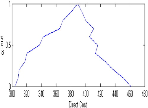
Here the total transportation amount is almost equal (since $\sum {\tilde{a}}_i=\sum {\tilde{b}}_j=\sum {\tilde{e}}_k$). Here GA produces a realistic scenario of most of the nonzero solution. For different values of $\alpha$, the optimal quantity $x_{ijk}$ is different for which per unit cost change in a normal range, as shown in Figure 5.

Figure 5. Direct Transportation Cost Vs $\alpha$-Cut.

Case-2: Now, we consider the values of the origins(i.e. sources), destination (i.e. demands) and conveyance(i.e. capacity) are taken as scrips number and The availability of the sources, demand of the destinations and capacity of the conveyances are as follows: $a_1=50,$ $a_2=30,$ $b_1=30,$ $b_2=50,$ $e_1=25,$, $e_2=55.$. With this inputs and other same input data, GA is performed for the objective function given in equation(10) subject to the constraints (11)-(14) as stated earlier using above mentioned GAs. The optimum results are presented below:

7. Discussion

Here, the final output (optimum amount of transportation and optimum profit) of the proposed model for different discrete value of $\alpha -$Cut is shown in Tables 3 and 4. From both Tables 3 and 4 it is observed that

• For Case-1, the total amount of transportation $\sum _{i=1}^M\sum _{j=1}^N\sum _{k=1}^K{x}_{ijk}$ lies between Max{$({\tilde{a}}_1+{\tilde{a}}_2{)}_L$, $({\tilde{b}}_1+{\tilde{b}}_2{)}_L$,($({\tilde{e}}_1+{\tilde{e}}_2{)}_L$} and Min{$({\tilde{a}}_1+{\tilde{a}}_2{)}_U$,$({\tilde{b}}_1+{\tilde{b}}_2{)}_U$, $({\tilde{e}}_1+{\tilde{e}}_2{)}_U$}.

• In Case-1, total amount of transportation does not tally with total cost or profit due to the existence of discount on unit of transportation. As the amount of transportation is fixed, so total amount of transportation does tally with total cost or profit in Case-2 which in Table 4.

• From Figure 5, it is also revels that the direct transportation cost function is convex with respect to $\alpha$

Table 3. Optimum Result of Case-1.

Value of α	Transportable Amounts x111 x121 x112 x122 x211 x221 x212 x222	PLα	PUα	Pc
1.0	8.3, 12.5, 27.5, 1.5, 5.1, 0.3, 12.0, 10.7	535.6	535.6	535.6
0.9	7.2, 12.2, 27.2, 2.3, 5.0, 0.2, 13.0, 10.1	529.2	542.3	535.7
0.8	7.7, 10.2, 27.3, 2.9, 3.9, 0.1, 13.5, 10.9	520.7	546.8	533.8
0.7	7.8, 14.5, 26.2, 0.0, 5.0, 10.1, 13.7, 0.0	529.1	570.3	549.7
0.6	10.5, 14.7, 24.0, 0.4, 6.6, 11.1, 11.0, 0.0	543.2	597.8	570.5
0.5	10.4, 13.0, 25.5, 0.0, 5.6, 0.4, 12.2, 11.8	548.0	616.8	582.4
0.4	11.2, 11.5, 25.6, 0.3, 4.5, 0.3, 12.0, 12.3	535.5	614.9	575.2
0.3	11.8, 11.6, 23.4, 2.0, 4.4, 0.0, 13.9, 10.9	533.5	628.5	581.0
0.2	11.8, 11.1, 26.7, 0.4, 4.3, 14.3, 11.2, 0.0	554.2	666.1	610.1
0.1	0.0, 12.2, 26.5, 10.4, 15.7, 2.6, 11.6, 0.0	535.4	661.5	598.4
0.0	3.6, 11.9, 23.2, 10.3, 17.2, 2.2, 10.6, 0.0	526.9	665.1	596.0

Table 4. Optimum Result of Case-2.

Value of α	Transportable Amounts x111x121x112x122x211x221x212x222	PLα	PUα	Pc
1.0	0.0, 17.5, 21.2, 11.3, 0.0, 7.5, 8.8, 13.7	521.1	664.1	592.6
0.9	0.0, 17.5, 21.2, 11.3, 0.0, 7.5, 8.8, 13.7	525.2	653.9	589.6
0.8	0.0, 17.5, 21.2, 11.3, 0.0, 7.5, 8.8, 13.7	529.3	643.7	586.5
0.7	0.0, 17.5, 21.2, 11.3, 0.0, 7.5, 8.8, 13.7	533.4	63.5	583.5
0.6	0.0, 17.5, 21.2, 11.3, 0.0, 7.5, 8.8, 13.7	537.5	623.3	580.4
0.5	0.0, 17.5, 21.2, 11.3, 0.0, 7.5, 8.8, 13.7	541.6	613.1	577.4
0.4	0.0, 17.5, 21.2, 11.3, 0.0, 7.5, 8.8, 13.7	545.7	602.9	574.3
0.3	0.0, 17.5, 21.2, 11.3, 0.0, 7.5, 8.8, 13.7	549.8	592.7	571.3
0.2	0.0, 17.5, 21.2, 11.3, 0.0, 7.5, 8.8, 13.7	553.9	582.5	568.2
0.1	0.0, 17.5, 21.2, 11.3, 0.0, 7.5, 8.8, 13.7	558	572.3	565.1
0.0	0.0, 17.5, 21.2, 11.3, 0.0, 7.5, 8.8, 13.7	562.1	562.1	562.1

8. Conclusions and Future Research Work

This paper is a wide extension of the paper proposed by Ojha et al. [8]. Here for the first time different type of vehicle costs are consider in a STP. The fixed charge, the unit transportation cost (under AUD) all are treated as fuzzy parameters. The problem is formulated as a profit maximisation problem. The budget constraint has been incorporated taking fuzzy unit transportation cost as constraint. To find the optimal solution genetic algorithm (a biological phenomena) is considered. The proposed model also can be extended for breakable items, defective items etc. This model also can be solved by other techniques like multi-objective genetic algorithm, goal programming, geometric programming, etc.

Disclosure statement

Here for the first time different type of vehicle costs are consider in a STP. The fixed charge, the unit transportation cost (under AUD) all are treated as fuzzy parameters. The problem is formulated as a profit maximization problem. The budget constraint has been incorporated taking fuzzy unit transportation cost as constraint.

Additional information

Notes on contributors

S. Samanta

Mr. S. Samanta is an Assistant Teacher of Mathematics at Majurhati Junior High School. He completed his graduation , PG and Ph.D. with under Vidyasagar University.

A. Ojha

Dr. A. Ojha is an Assistant Teacher of Mathematics at Siromoni Birsa Munda High School. He completed his graduation, PG and Ph.D. from Vidyasagar University. His research fields are Transportations and Soft Computing. He has some publications in different reputed international journals like Tamsui Oxford Journal of Management Science, Fuzzy Systems and Soft Computing, Mathematical and Computer Modelling, Applied Mathematical Modelling, Applied Soft Computing, etc.

B. Das

Dr. B. Das is an Associate Professor in the department of Mathematics at Sidhu Kanhu Birsha University. He completed his graduation with gold medal under Vidyasagar University. He completed his PG and Ph.D. from Vidyasagar University. His research fields are Biomathematics, Inventory, Soft Computing and Supply Chain. He has been doctoral dissertation adviser to 4 students as of now and 6 students are working currently under his supervision. He is working in this department from 2013 and previously he was working at Jhargram Raj College. He has more than 70 publications in different reputed international journals like Journal of Computational and Applied Mathematics, Asian Journal of Mathematics and Physics, Applied Mathematical and Computation, Mathematical and Computer Modelling, Applied Mathematical Modelling, Applied Soft Computing, Journal of Computational Science, Journal of Simulation, Computers & Industrial Engineering, Transportation Research Part E: Logistics and Transportation Review, Annals of Operations Research, etc. He was died last year due to covid 19.

S. K. Mondal

Prof. S. K. Mondal is Professor and HOD in the department of Applied Mathematics with Oceanology and Computer Programming at Vidyasagar University. He was gold medalist of Vidyasagar University at UG and PG level. He completed his M.Tech. degree from ISM dhanbad. He completed his Ph.D. degree from Vidysagar University. His research interest areas are Biomathematics, Inventory, Supply Chain, Soft computing and Risk analysis. He has been doctoral dissertation adviser to 14 students as of now and 6 students are working currently under his supervision and 4 has been faced their pre submission seminar. He is working in this department from 2004 and working as a professor till 2015. He visited Vietnam, Thailand and Bangladesh to deliver speech in different international conferences. He has more than 150 international publications in different reputed international journals like Journal of Cleaner Production, Transportation Research Part E: Logistics and Transportation Review, Applied Soft Computing, Journal of Industrial and Production Engineering, Computers & Industrial Engineering, Annals of Operations Research, Chaos, Solutions & Fractals, Information Sciences, Nonlinear Dynamics etc.

References

- He Y. Generalized Interval-valued atanassov’s intuitionistic fuzzy power operators and their application to multiple attribute group decision making. Int J Fuzzy Syst. 2013;15:401–411.
- He Y. Generalized intuitionistic fuzzy geometric interaction operators and their application to decision making. Expert Syst Appl. 2014;41:2484–2495.
- He Y. Hesitant fuzzy Power Bonferroni means and their Application to Multiple Attribute decision making. IEEE Trans Fuzzy Syst. 2015;23:1655–1668.
- Hitchcock FL. The distribution of a product from several sources to numerous localities. J Math Phys. 1941;20:224–230.
- Shell E. Distribution of a product by several properties. Direclorale of Management Analysis. Proceedings of the 2nd Symposium in Liner Programming; 2:615–642.
- Samanta S, Das B, Mondal SK. Multi-objective solid transportation problem with discount and two-level fuzzy programming technique. Int J Operat Res. 2015;24(4):423–440.
- Pan Y, Joo Er M. Enhanced adaptive fuzzy control with optimal approximation error convergence. IEEE Trans Fuzzy Syst. 2013;21(6):1123–1132.
- Ojha A, Das B, Mondal SK, et al. A solid transportation problem for an item with fixed charge, vechicle cost and price discounted varying charge using Genetic algorithm. Appl Soft Comput. 2010;10:100–110.
- Dalman H, Güzel N, Sivri M. A fuzzy Set-Based approach to multi-objective multi-item Solid Transportation Problem Under uncertainty. Int J Fuzzy Syst. 2015;18:716–729.
- Jimenez F, Verdegay JL. Uncertain solid transportation problem. Fuzzy Sets Syst. 1998;100:45–57.
- Chanas S, Kuchta D. A concept of the optimal solution of the transportation problem with fuzzy cost coefficients. Fuzzy Sets Syst. 1996;82:299–305.
- Li L, Lai KK. A fuzzy approach to the multi-objective transportation problem. Comput Operat Res. 2000;27:43–57.
- Bit AK, Biswal MP, Alam SS. An additive fuzzy programming model for multi-objective transportation problem. Fuzzy Sets Syst. 1993;57:313–319.
- Jimencz F, Verdegay JL. Interval multiobjective solid transportation problem via Genetic algorithms. Management of Uncertainty in Knowledge-Based Systems II. 1996: 787–792.
- Das SK, Goswami A, Alam SS. Multi-objective transportation problem with interval cost,source and destination parameters. Eur J Oper Res. 1999;117:100–112.
- Abd El-Wahed WF. A multi-objective transportation problem under fuzziness. Fuzzy Sets Syst. 2001;117:27–33.
- Grzegorzewski P. Nearest interval approximation of a fuzzy number. Fuzzy Sets Syst. 2002;130:321–330.
- Saad OM, Abass SA. A parametric study on transportation problem under fuzzy environment. J Fuzzy Mathemat. 2003;11(1):115–124.
- Ojha A, Das B, Mondal SK, et al. An entropy based solid transportation problem for General fuzzy costs and time with fuzzy equality. Math Comput Model. 2009;50:166–178.
- Huang T. Fuzzy multilevel Lot-sizing problem Based on Signed distance and centroid. Int J Fuzzy Syst. 2011;13(2):98–110.
- Sakawaa M, Nishizakia I, Uemurab Y. Fuzzy programming and profit and cost allocation for a production and transportation problem. Eur J Oper Res. 2001;131(1):1–15.
- Pan Y, Joo Er M, Li X. Haoyong Yu and rafael gouriveau “Machine health condition prediction via online dynamic fuzzy neural networks”. Eng Appl Artif Intell. 2014;35:105–113.
- Ojha A, Das B, Mondal SK, et al. A stochastic discounted multi-objective solid transportation problem for breakable items using analytical hierarchy process. Appl Math Model. 2010;34(8):2256–2271.
- Goldberg D. Genetic algorithms in search, optimization and machine learning. MA: Addision Wealey; 1989.
- Ju Wu C, Ko C-N, Fu Y-Y, et al. A genetic-Based design of auto-tuning fuzzy PID controllers. Int J Fuzzy Syst. 2009;11(1):49–58.
- Basu M, Pal BB, Kundu A. An algorithm for finding the optimum solution of solid fixed charge transportation problem. Optimization. 1994;31(3):283–291.
- Maiti AK, Maiti M. Discounted multi-item inventory model via Genetic Algorithm with roulette wheel section, arithmetic crossover and uniform mutation in constraints bounded domains. Int J Comput Math. 2008;85(9):1341–1353.
- Vignaux GA, Michalewicz Z. A genetic algorithm for the liner transpotation problem. IEEE Trans Syst Man Cybern. 1991;21(2):445–452.
- Liu L, Lin L. Fuzzy fixed charge solid transportation problem and its algorithm. Fuzzy Syst Knowlege Discov. 2007;3:585–589.