Output Feedback Controller for a Class of Unknown Nonlinear Discrete Time Systems Using Fuzzy Rules Emulated Networks and Reinforcement Learning

Abstract

A model-free adaptive control for non-affine discrete time systems is developed by utilising the output feedback and action-critic networks. Fuzzy rules emulated network (FREN) is employed as the action network and multi-input version (MiFREN) is implemented as the critic network. Both networks are constructed using human knowledge based on IF–THEN rules according to the controlled plant and the learning laws are established by reinforcement learning without any off-line learning phase. The theoretical derivation of the convergence of the tracking error and internal signal is demonstrated. The numerical simulation and the experimental system are given to validate the proposed scheme.

Keywords:

• Model-free adaptive control
• reinforcement learning
• nonlinear discrete time systems
• fuzzy neural network
• DC motor current control

1. Introduction

Due to the complexity of controlled plants nowadays, it is commonly difficult or impossible to establish its mathematical model especially for the discrete time system [1]. By utilising only input–output data of the controlled plant, the model-free approaches have been developed [2, 3]. On the other hand, the performance of the controllers is related to data's quality and quantity [4]. For some engineering applications, it is very difficult to access all state variables, thus the output feedback is still a preferable scheme [5, 6]. Furthermore, the close-loop analysis and stability approaches have been proposed [7, 8, 9] to guarantee the performance of controllers. From the engineering point of view, the stability analysis beside of closed-loop's performance is only a basic minimum requirement even for the artificial intelligence controller [10]. Therefore, the optimal controllers are more desirable for modern applications [11] or by nature view [12].

To ensure the closed-loop performance with the optimisation of the predefined cost function, the schemes based on adaptive dynamic programming have been utilised but the mathematic models have been required for its iterative learning [13, 14]. With the model-free aspects, reinforcement learning (RL) algorithms have been developed to solve optimal control [15, 16] with the estimated solution of the Hamilton–Jacobi–Bellman equation [17, 18]. To mimic the RL process, the approaches based on action-critic networks have been derived by artificial neural networks ( ANNs) under considering the controlled plant as a black box [19, 20]. Nevertheless, even the mathematic model is unknown but the engineer still has basic human knowledge of the controlled plant such that ‘IF higher output is required THEN more control effort should be supplied’. Thus, the controlled plant can be considered as a grey box.

To integrate the human knowledge as IF–THEN format into the controller, fuzzy logic systems ( FLSs) have been utilised in control applications [21] also including the optimal problems [22]. By including the learning ability to FLS, the integrations between FLS and ANN have been developed such as fuzzy neural network (FNN) [23] and fuzzy rules emulated network (FREN) [24, 25]. Thereafter, the approaches of using FNN and FREN for solving the optimal problem with RL have been proposed [26, 27] when the controlled plants have been considered as a class of affine systems. On the other hand, the problem of non-affine systems has been studied in Ref. [28] by the approach of critic-action networks when the state feedback has been utilised for gaining enough information to tune ANNs.

In this work, the output feedback model-free controller is proposed when the control effort is non-affine with respect to system dynamics. The controller is designed by the action network called FRENa with the set of IF–THEN rules according to the controlled plant. Thereafter, the long-term cost function is estimated by the multi-input version of FREN called MiFRENc when IF–THEN rules are established under the general aspect for minimising both tracking error and control energy. The learning laws are derived with the RL approach to tune all adjustable parameters of FRENa and MiFRENc aiming to minimise the tracking error and the estimated cost function. Furthermore, the closed-loop analysis is provided by the Lyapunov method to demonstrate the convergence of the tracking error and internal signals.

This paper is organised as follows. Section 2 introduces a class of systems under our investigation and problem formulation. The proposed scheme is introduced in Section 3 including the network architectures with IF–THEN rules of FRENa and MiFRENc and their formulations. The learning laws and closed-loop analysis are derived in Section 4. Section 5 provides the results of the simulation and experimental system.

2. Controlled Plant as a Class of Nonlinear Discrete-Time Systems

In this work, the controlled plant for a class of non-affine discrete time systems is considered as (1) $y(k+1)=f(y(k),\dots ,y(k-n_y),u(k),\dots ,u(k-n_u))+d(k),$(1) where $y(k+1)\in \mathbb{R}$ is the plant's output with respect to the control effort $u(k)\in \mathbb{R}$, $f(-)$ is an unknown nonlinear function, $n_u$ and $n_y$ are unknown system orders and $d(k)$ denotes a bounded disturbance such that $|d(k)|\le d_M$. For further analysis, the following assumptions are expressed according to the unknown nonlinear function $f(-)$ with respect to the control effort $u(k)$.

Assumption 2.1

The derivative of $y(k+1)$ with respect to $u(k)$ is existed and bounded such that (2) $0<g_m\le \frac{\mathrm{\partial }y(k+1)}{\mathrm{\partial }u(k)}\le g_M,$(2) where $g_m$ and $g_M$ are positive constants.

Remark 2.2

The condition mentioned in (2(2) $0<g_m\le \frac{\mathrm{\partial }y(k+1)}{\mathrm{\partial }u(k)}\le g_M,$(2) ) indicates that the controlled plant in (1(1) $y(k+1)=f(y(k),\dots ,y(k-n_y),u(k),\dots ,u(k-n_u))+d(k),$(1) ) is a positive control direction. That will assist the setting of IF–THEN rules according to the change of control effort $\mathrm{\Delta }u(k)$ altogether with the change of output $\mathrm{\Delta }y(k+1)$.

Referring to condition (2(2) $0<g_m\le \frac{\mathrm{\partial }y(k+1)}{\mathrm{\partial }u(k)}\le g_M,$(2) ), it is clear that the change of output $\mathrm{\Delta }y(k+1)$ with respect to the change of control effort $\mathrm{\Delta }u(k)$ can be rewritten as (3) $g_m^d\le \frac{\mathrm{\Delta }y(k+1)}{\mathrm{\Delta }u(k)}\le g_M^d,$(3) where $\mathrm{\Delta }u(k)>0$ and $g_m^d$ and $g_M^d$ are constants according to $g_m$ and $g_M$, respectively. This will lead to the setting of IF–THEN rules such that

IF $\mathrm{\Delta }u(k)$ is positive-large, THEN $\mathrm{\Delta }y(k+1)$ should be positive-large

or

IF $\mathrm{\Delta }u(k)$ is negative small, THEN $\mathrm{\Delta }y(k+1)$ should be negative small.

By utilising those IF–THEN rules, the adaptive controller based on FRENs will be established in the next section.

3. RL Controller

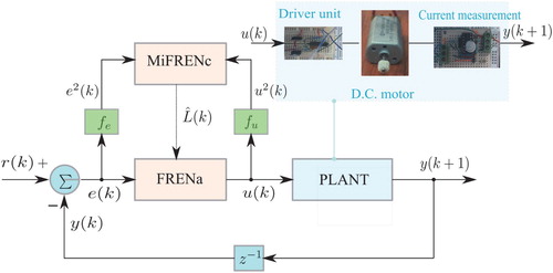
The proposed controller is illustrated by the block diagram in Figure 1. In this work, the plant is selected as a DC motor current control. Only the armature current is measured as the output $y(k+1)$ (mA) when the control effort $u(k)$ (V) is the voltage fed to the driver unit. Thus, the IF–THEN rules mentioned in Section 2 can be rewritten according to the physical nature such that

Figure 1. Closed-loop system architecture.

IF we apply positive-large change of control voltage [$\mathrm{\Delta }u(k)$], THEN we should have positive-large change of armature current [$\mathrm{\Delta }y(k+1)$].

According to this knowledge, the action network (FRENa) is first established to generate the control effort $y(k)$ when the input is the tracking error $e(k)$ defined as (4) $e(k)=r(k)-y(k),$(4) where $r(k)$ is the desired trajectory. Second, the critic network is designed using MiFRENc to produce the estimated long-term cost function $\hat{L}(k)$ for the controller FRENa. The details of two networks and its IF–THEN rules are given as follows.

3.1. Controller or Action Network

To utilise the action network, the IF–THEN rules with the relation between the tracking error $e(k)$ and the control effort $u(k)$ are first established. By considering the basic knowledge such that, positive-large $e(k)$ means lack of $y(k)$ in positive-large. In order to compensate, it clearly requires that the control effort $u(k)$ should be positive-large. For conclusion, we have IF $e(k)$ is positive-large, THEN $u(k)$ should be positive-large. With seven linguistic levels, it leads to the design of IF–THEN rules as

Table

IF $e(k)$ is NL	THEN $u(k)$ is NL,
IF $e(k)$ is NM	THEN $u(k)$ is NM,
IF $e(k)$ is NS	THEN $u(k)$ is NS,
IF $e(k)$ is Z	THEN $u(k)$ is Z,
IF $e(k)$ is PS	THEN $u(k)$ is PS,
IF $e(k)$ is PM	THEN $u(k)$ is PM,
IF $e(k)$ is PL	THEN $u(k)$ is PL,

where notations of linguistic variables N, P, L, M, S and Z denote negative, positive, large, medium, small and zero, respectively.

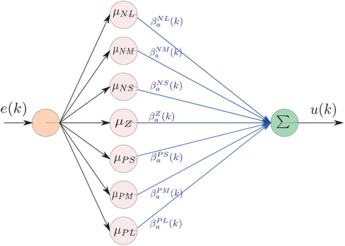
Employing this set of IF–THEN rules, the network architecture of FRENa is illustrated by Figure 2. According to the network architecture in Figure 2 and the function formulation of FREN in Ref. [24], the control effort $u(k)$ is determined by (5) $u(k)={\beta }_a^T(k){\varphi }_a(k),$(5) where (6) ${\varphi }_a(k)=[{\mu }_{\mathrm{NL}}(e_k){\mu }_{\mathrm{NM}}(e_k)\cdots {\mu }_{\mathrm{PL}}(e_k){]}^T$(6) and (7) ${\beta }_a(k)=[{\beta }_a^{\mathrm{NL}}(k){\beta }_a^{\mathrm{NM}}(k)\cdots {\beta }_a^{\mathrm{PL}}(k){]}^T.$(7)

Figure 2. Action network or controller based on FREN.

Let us consider FRENa as the function estimator of the unknown control effort, thus it exists the ideal control effort $u^{\ast }(k)$ with the ideal parameter ${\beta }_a^{\ast }$ such that (8) $u^{\ast }(k)={\beta }_a^{\ast T}{\varphi }_a(k)+{\epsilon }_a(k),$(8) where ${\epsilon }_a(k)$ is a bounded residual error $|{\epsilon }_a(k)|\le {\epsilon }_{aM}$.

By using the dynamics (1(1) $y(k+1)=f(y(k),\dots ,y(k-n_y),u(k),\dots ,u(k-n_u))+d(k),$(1) ) with the control laws (5(5) $u(k)={\beta }_a^T(k){\varphi }_a(k),$(5) ) and (8(8) $u^{\ast }(k)={\beta }_a^{\ast T}{\varphi }_a(k)+{\epsilon }_a(k),$(8) ), the tracking error $e(k+1)$ is rearranged as (9) $\begin{array}{rl}e(k+1)& =r(k+1)-y(k+1)\\ & =f(u_k^{\ast })-f(u_k)-d(k).\end{array}$(9) Recalling Assumption 1 and using mean value theorem, the error dynamic (9(9) $\begin{array}{rl}e(k+1)& =r(k+1)-y(k+1)\\ & =f(u_k^{\ast })-f(u_k)-d(k).\end{array}$(9) ) can be rewritten as (10) $\begin{array}{rl}e(k+1)& =\frac{\mathrm{\partial }f(x)}{\mathrm{\partial }x}{|}_{x=u^m(k)}[u^{\ast }(k)-u(k)]-d(k)\\ & =g(k)[u^{\ast }(k)-u(k)]-d(k),\end{array}$(10) where (11) $g(k)=\frac{\mathrm{\partial }f(u^m(k))}{\mathrm{\partial }{u}^m(k)},$(11) and $u^m(k)\in [min\{u_k^{\ast },u_k\},max\{u_k^{\ast },u_k\}]$. Employing the control laws (8(8) $u^{\ast }(k)={\beta }_a^{\ast T}{\varphi }_a(k)+{\epsilon }_a(k),$(8) ) and (5(5) $u(k)={\beta }_a^T(k){\varphi }_a(k),$(5) ), it yields (12) $e(k+1)=g(k)[{\beta }_a^{\ast }-{\beta }_a(k){]}^T{\varphi }_a(k)+g(k){\epsilon }_a(k)-d(k).$(12) Let us define ${\tilde{\beta }}_a(k)={\beta }_a^{\ast }-{\beta }_a(k)$, $d_a(k)=g(k){\epsilon }_a(k)-d(k)$ and (13) ${\mathrm{\Lambda }}_a(k)={\tilde{\beta }}_a^T(k){\varphi }_a(k),$(13) and we obtain (14) $e(k+1)=g(k){\mathrm{\Lambda }}_a(k)+d_a(k).$(14) It is worth to note that the tracking error obtained by (14(14) $e(k+1)=g(k){\mathrm{\Lambda }}_a(k)+d_a(k).$(14) ) is functional by ${\tilde{\beta }}_a(k)$ and the unknown but bounded $d_a(k)$ such that $|d_a(k)|\le d_{aM}$. This relation will be used for the performance analysis afterward.

3.2. Estimated Cost–Function or Critic Network

In this work, the long-term cost function $L(k)$ is employed by an infinite-horizon of the tracking error $e(k)$ and the control effort $u(k)$ with the discount factor ${\gamma }_L$ as (15) $L(k)=\sum _{i=k}^{\mathrm{\infty }}{\gamma }_L^{i-k}l(i),$(15) where (16) $l(k)=p{e}^2(k)+q{u}^2(k),$(16) where p and q are positive constants and $0<{\gamma }_L\le 1$.

$L(k)$ in (15(15) $L(k)=\sum _{i=k}^{\mathrm{\infty }}{\gamma }_L^{i-k}l(i),$(15) ) is functional by two input arguments with the quadratic functions ($f_x=x^2$) of $e(k)$ and $u(k)$. Thus, an adaptive network MiFRENc is utilised to estimate $L(k)$ as the block diagram in Figure 1. In order to design MiFRENc, IF–THEN rules are first established by Table 1. Thereafter, the network architecture of MiFRENc is illustrated by Figure 3. By utilising the network in Figure 3 and results in Ref. [24], the estimated cost function $\hat{L}(k)$ is determined by (17) $\hat{L}(k)={\beta }_c^T(k){\varphi }_c(k),$(17) where (18) ${\beta }_c(k)=[{\beta }_{\mathrm{ZZ}}(k){\beta }_{\mathrm{ZS}}(k)\cdots {\beta }_{\mathrm{LL}}(k){]}^T$(18) and (19) ${\varphi }_c(k)=[{\varphi }_1(k){\varphi }_2(k)\cdots {\varphi }_9(k){]}^T.$(19)

Figure 3. Estimated cost function or critic network.

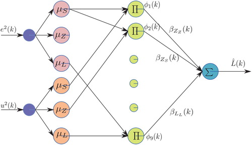
Table 1. MiFRENc: IF–THEN rules.

	$e^2(k)$
$\hat{L}(k)$		Z	S	L
$u^2(k)$	Z	${\varphi }_1;$ Z${}_{\mathrm{Z}}$	${\varphi }_4;$ S${}_{\mathrm{Z}}$	${\varphi }_7;$L${}_{\mathrm{Z}}$
	S	${\varphi }_2;$ Z${}_{\mathrm{S}}$	${\varphi }_5;$ S${}_{\mathrm{S}}$	${\varphi }_8;$L${}_{\mathrm{S}}$
	L	${\varphi }_3;$ Z${}_{\mathrm{L}}$	${\varphi }_6;$ S${}_{\mathrm{L}}$	${\varphi }_9;$L${}_{\mathrm{L}}$

Using the universal approximation property of MiFREN [24], there exists an ideal parameter ${\beta }_c^{\ast }$ such that (20) $L(k)={\beta }_c^{\ast T}{\varphi }_c(k)+{\epsilon }_c(k),$(20) where ${\epsilon }_c(k)$ is a bounded residual error such that $|{\epsilon }_c(k)|\le {\epsilon }_{cM}$. Adding and subtracting ${\beta }_c^{\ast T}{\varphi }_c(k)$ on the left-hand side of (17(17) $\hat{L}(k)={\beta }_c^T(k){\varphi }_c(k),$(17) ) yields (21) $\begin{array}{rl}\hat{L}(k)& ={\tilde{\beta }}_c^T(k){\varphi }_c(k)+{\beta }_c^{\ast T}{\varphi }_c(k)\\ & ={\mathrm{\Lambda }}_c(k)+{\beta }_c^{\ast T}{\varphi }_c(k),\end{array}$(21) where ${\tilde{\beta }}_c(k)={\beta }_c^T(k)-{\beta }_c^{\ast }$ and ${\mathrm{\Lambda }}_c(k)={\tilde{\beta }}_c^T(k){\varphi }_c(k)$.

In order to improve the performance of FRENa and MiFRENc, the learning laws will be developed and explained in the next section.

4. Learning Algorithms and Performance Analysis

4.1. Action Network Learning Law

Considering the tracking error within ${\mathrm{\Lambda }}_a(k)$ as (14(14) $e(k+1)=g(k){\mathrm{\Lambda }}_a(k)+d_a(k).$(14) ) and the estimated cost function $\hat{L}(k)$, in this work, the error function of action network is given as (22) $e_a(k)=\sqrt{g(k)}{\mathrm{\Lambda }}_a(k)+\frac{1}{\sqrt{g(k)}}\hat{L}(k).$(22) Thereafter, the cost function to be minimised is utilised as (23) $E_a(k)=\frac{1}{2}{e}_a^2(k).$(23) Applying the gradient descent, the tuning law for ${\beta }_a$ is derived as (24) ${\beta }_a(k+1)={\beta }_a(k)-{\eta }_a\frac{\mathrm{\partial }{E}_a(k)}{\mathrm{\partial }{\beta }_a(k)},$(24) where ${\eta }_a$ is the learning rate. By using the chain rule and (13(13) ${\mathrm{\Lambda }}_a(k)={\tilde{\beta }}_a^T(k){\varphi }_a(k),$(13) ), it yields (25) $\begin{array}{rl}\frac{\mathrm{\partial }{E}_a(k)}{\mathrm{\partial }{\beta }_a(k)}& =\frac{\mathrm{\partial }{E}_a(k)}{\mathrm{\partial }{e}_a(k)}\frac{\mathrm{\partial }{e}_a(k)}{\mathrm{\partial }{\mathrm{\Lambda }}_a(k)}\frac{\mathrm{\partial }{\mathrm{\Lambda }}_a(k)}{\mathrm{\partial }{\beta }_a(k)}\\ & =-e_a(k)\sqrt{g(k)}{\varphi }_a(k).\end{array}$(25) Recalling (24(24) ${\beta }_a(k+1)={\beta }_a(k)-{\eta }_a\frac{\mathrm{\partial }{E}_a(k)}{\mathrm{\partial }{\beta }_a(k)},$(24) ) with (25(25) $\begin{array}{rl}\frac{\mathrm{\partial }{E}_a(k)}{\mathrm{\partial }{\beta }_a(k)}& =\frac{\mathrm{\partial }{E}_a(k)}{\mathrm{\partial }{e}_a(k)}\frac{\mathrm{\partial }{e}_a(k)}{\mathrm{\partial }{\mathrm{\Lambda }}_a(k)}\frac{\mathrm{\partial }{\mathrm{\Lambda }}_a(k)}{\mathrm{\partial }{\beta }_a(k)}\\ & =-e_a(k)\sqrt{g(k)}{\varphi }_a(k).\end{array}$(25) ) and using $e_a(k)$ in (22(22) $e_a(k)=\sqrt{g(k)}{\mathrm{\Lambda }}_a(k)+\frac{1}{\sqrt{g(k)}}\hat{L}(k).$(22) ), it leads to (26) $\begin{array}{rl}{\beta }_a(k+1)& ={\beta }_a(k)+{\eta }_a{e}_a(k)\sqrt{g(k)}{\varphi }_a(k)\\ & ={\beta }_a(k)+{\eta }_a[\sqrt{g(k)}{\mathrm{\Lambda }}_a(k)+\frac{1}{\sqrt{g(k)}}\hat{L}(k)]\sqrt{g(k)}{\varphi }_a(k)\\ & ={\beta }_a(k)+{\eta }_a[g(k){\mathrm{\Lambda }}_a(k)+\hat{L}(k)]{\varphi }_a(k).\end{array}$(26) By eliminating $d_a(k)$ in (14(14) $e(k+1)=g(k){\mathrm{\Lambda }}_a(k)+d_a(k).$(14) ), the learning law (26(26) $\begin{array}{rl}{\beta }_a(k+1)& ={\beta }_a(k)+{\eta }_a{e}_a(k)\sqrt{g(k)}{\varphi }_a(k)\\ & ={\beta }_a(k)+{\eta }_a[\sqrt{g(k)}{\mathrm{\Lambda }}_a(k)+\frac{1}{\sqrt{g(k)}}\hat{L}(k)]\sqrt{g(k)}{\varphi }_a(k)\\ & ={\beta }_a(k)+{\eta }_a[g(k){\mathrm{\Lambda }}_a(k)+\hat{L}(k)]{\varphi }_a(k).\end{array}$(26) ) is rewritten as (27) ${\beta }_a(k+1)={\beta }_a(k)+{\eta }_a[e(k+1)+\hat{L}(k)]{\varphi }_a(k).$(27) The final learning law of FRENa given by (27(27) ${\beta }_a(k+1)={\beta }_a(k)+{\eta }_a[e(k+1)+\hat{L}(k)]{\varphi }_a(k).$(27) ) is a practical one because all parameters required on the left-hand side are certainly obtained at the time index k + 1.

4.2. Critic Network Learning Law

In general, the error function of critic networks is employed by the estimated cost function $\hat{L}(k)$. Therefore, in this work, the error function $e_c(k)$ is given as (28) $e_c(k)=\delta \hat{L}(k)-\hat{L}(k-1)+l(k),$(28) where δ is a positive constant. In order to tune ${\beta }_c$, the cost function $E_c(k)$ is defined as (29) $E_c(k)=\frac{1}{2}{e}_c^2(k).$(29) Applying the gradient descent at (29(29) $E_c(k)=\frac{1}{2}{e}_c^2(k).$(29) ) with respect to ${\beta }_c(k)$, we have (30) ${\beta }_c(k+1)={\beta }_c(k)-{\eta }_c\frac{\mathrm{\partial }{E}_c(k)}{\mathrm{\partial }{\beta }_c(k)},$(30) where ${\eta }_c$ is the learning rate. Using the chain rule along $E_c(k)$ in (29(29) $E_c(k)=\frac{1}{2}{e}_c^2(k).$(29) ), $e_c(k)$ in (28(28) $e_c(k)=\delta \hat{L}(k)-\hat{L}(k-1)+l(k),$(28) ) and $\hat{L}(k)$ in (17(17) $\hat{L}(k)={\beta }_c^T(k){\varphi }_c(k),$(17) ), it yields (31) $\begin{array}{rl}\frac{\mathrm{\partial }{E}_c(k)}{\mathrm{\partial }{\beta }_c(k)}& =\frac{\mathrm{\partial }{E}_c(k)}{\mathrm{\partial }{e}_c(k)}\frac{\mathrm{\partial }{e}_c(k)}{\mathrm{\partial }\hat{L}(k)}\frac{\mathrm{\partial }\hat{L}(k)}{\mathrm{\partial }{\beta }_c(k)}\\ & =e_c(k)\delta {\varphi }_c(k).\end{array}$(31) Rewriting (30(30) ${\beta }_c(k+1)={\beta }_c(k)-{\eta }_c\frac{\mathrm{\partial }{E}_c(k)}{\mathrm{\partial }{\beta }_c(k)},$(30) ) with (31(31) $\begin{array}{rl}\frac{\mathrm{\partial }{E}_c(k)}{\mathrm{\partial }{\beta }_c(k)}& =\frac{\mathrm{\partial }{E}_c(k)}{\mathrm{\partial }{e}_c(k)}\frac{\mathrm{\partial }{e}_c(k)}{\mathrm{\partial }\hat{L}(k)}\frac{\mathrm{\partial }\hat{L}(k)}{\mathrm{\partial }{\beta }_c(k)}\\ & =e_c(k)\delta {\varphi }_c(k).\end{array}$(31) ), it leads to (32) $\begin{array}{rl}{\beta }_c(k+1)& ={\beta }_c(k)-{\eta }_c{e}_c(k)\delta {\varphi }_c(k)\\ & ={\beta }_c(k)-{\eta }_c\delta [l(k)-\hat{L}(k-1)+\delta \hat{L}(k)]{\varphi }_c(k).\end{array}$(32) Finally, we have a practical tuning law for MiFRENc.

4.3. Closed-Loop Analysis

In the following theorem, the closed-loop performance of the output feedback controller is demonstrated while the tracking error and internal signals are bounded.

Theorem 4.1

For the non-affine discrete time system mentioned in Section 2, the performance of the closed-loop system configured by the structure of FRENa and MiFRENc in Section 3 is guaranteed in terms of the bonded tracking error and internal signals when the designed parameters are selected as follows: (33) $\begin{array}{rl}& \frac{1}{2}<\delta \le 1,\end{array}$(33) (34) $\begin{array}{rl}& 0<{\eta }_a\le \frac{g_m}{{\nu }_a{g}_M^2}\end{array}$(34) and (35) $0<{\eta }_c\le \frac{1}{{\nu }_c{\delta }^2},$(35) where ${\nu }_a$ and ${\nu }_c$ are upper limits of $||{\varphi }_a(k)|{|}^2$ and $||{\varphi }_c(k)|{|}^2$, respectively.

Proof : The proof is given in Appendix.

The validation of the proposed control scheme will be presented in the next section for the computer simulation system with a non-affine discrete time system and the hardware implementation system for DC motor current control plant.

5. Simulation and Experimental Systems

5.1. Simulation System and Results

The controller developed in this work is first implemented on the nonlinear discrete time given as (36) $y(k+1)=\sin (y_k)+[5+\cos (y_k{u}_k)]u(k).$(36) It is worth to mention that the mathematic model in (36(36) $y(k+1)=\sin (y_k)+[5+\cos (y_k{u}_k)]u(k).$(36) ) is used only to establish the simulation. In this test, the desired trajectory is given as (37) $r(k+1)=A_r\sin \left({\omega }_r\pi \frac{k}{k_M}\right),$(37) where $k_M=500$ as the maximum time index, $A_r=1.0$ and ${\omega }_r=8$. To follow (33(33) $\begin{array}{rl}& \frac{1}{2}<\delta \le 1,\end{array}$(33) ), δ is selected as $\delta =0.75$ and ${\nu }_a={\nu }_c=1.5$. By using this setting and (35(35) $0<{\eta }_c\le \frac{1}{{\nu }_c{\delta }^2},$(35) ), the learning rate of MiFRENc is determined as (38) $0<{\eta }_c\le \frac{1}{{\delta }^2{\nu }_c^2}=\frac{1}{{0.75}^2{1.5}^2}=\mathrm{0.7901.}$(38) In this case, the learning rate for MiFRENc is selected as ${\eta }_c=0.5$. To select the learning rate of FRENa, let us chose $g_m$ and $g_M$ as 1 and 6, respectively. By using (34(34) $\begin{array}{rl}& 0<{\eta }_a\le \frac{g_m}{{\nu }_a{g}_M^2}\end{array}$(34) ), the learning rate of FRENa is determined as (39) $0<{\eta }_a\le \frac{g_m}{{\nu }_a^2{g}_M^2}=\frac{1}{{1.5}^2{6}^2}=\mathrm{0.0123.}$(39) Thus, the learning rate for FRENa is selected as ${\eta }_a=0.01$.

Figures 4 and 5 illustrate the setting of membership functions for FRENa and MiFRENc, respectively. The initial setting of adjustable parameters ${\beta }_{◻}(1)$ for FRENa and MiFRENc is given as Table 2.

Figure 4. FRENa membership functions: simulation case.

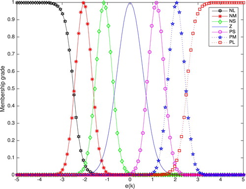
Figure 5. MiFRENc membership functions: simulation case.

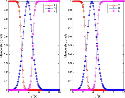
Table 2. Initial setting ${\beta }_{◻}(1)$: simulation system.

FRENa		MiFRENc
Parameter	Value	Parameter	Value
${\beta }_{\mathrm{NL}}(1)$	−0.25	${\beta }_{\mathrm{ZZ}}(1)$	0
${\beta }_{\mathrm{NM}}(1)$	−0.15	${\beta }_{\mathrm{ZS}}(1)$	0.1
${\beta }_{\mathrm{NS}}(1)$	−0.05	${\beta }_{\mathrm{ZL}}(1)$	0.2
${\beta }_{\mathrm{Z}}(1)$	0	${\beta }_{\mathrm{SZ}}(1)$	0.3
${\beta }_{\mathrm{PS}}(1)$	0.05	${\beta }_{\mathrm{SS}}(1)$	0.4
${\beta }_{\mathrm{PM}}(1)$	0.15	${\beta }_{\mathrm{SL}}(1)$	0.5
${\beta }_{\mathrm{PL}}(1)$	0.25	${\beta }_{\mathrm{LZ}}(1)$	0.6
		${\beta }_{\mathrm{LS}}(1)$	0.7
		${\beta }_{\mathrm{LL}}(1)$	0.8

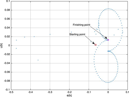
Figure 6 displays the tracking performance with both plots of $y(k)$ and $e(k)$ and Figure 7 represents the control effort $u(k)$. The estimated cost function $\hat{L}(k)$ is illustrated in Figure 8. The phase plane trajectory of $u(k)$ and $e(k)$ is depicted in Figure 9 to demonstrate the closed-loop system's behaviour.

Figure 6. Tracking performance $y(k)$ and $e(k)$: simulation system.

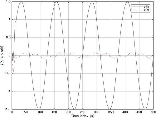
Figure 7. Control effort $u(k)$: simulation system.

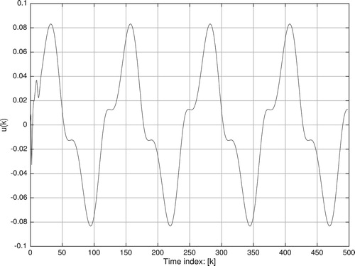
Figure 8. Estimated cost function $\hat{L}(k)$: simulation system.

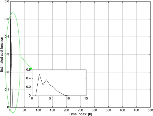
Figure 9. $u(k)$ and $e(k)$: simulation system.

5.2. Experimental System and Results

The experimental system is constructed by a DC motor current control. The output $y(k+1)$ is the armature current (mA) and the input $u(k)$ is the control voltage applied to the driver circuit depicted in Figure 1. Same as the simulation systems, let us select $\delta =0.75$, ${\nu }_a={\nu }_c=1.5$, $g_m=5$ and $g_M=10$. Thus, the learning rate of FRENa is designed as (40) $0<{\eta }_a\le \frac{g_m}{{\nu }_a^2{g}_M^2}=\frac{5}{{1.5}^2{10}^2}=\mathrm{0.0222.}$(40) In this case, we select ${\eta }_a=0.01$. For MiFRENc, we use the same learning rate as the simulation system such that ${\eta }_c=0.5$ because of the same network architecture. The desired trajectory is given as (41) $r(k+1)=I_r\sin \left({\omega }_r\pi \frac{k}{k_M}\right),$(41) where (42) $\begin{array}{rl}{I}_r& =\{\begin{array}{ll}15(\mathrm{mA})& \mathrm{if}0⩽k<\frac{k_M}{2},\\ 30(\mathrm{mA})& \mathrm{otherwise},\end{array}\end{array}$(42) (43) $\begin{array}{rl}{\omega }_r& =\{\begin{array}{ll}8& \mathrm{if}0⩽k<\frac{k_M}{2},\\ 4& \mathrm{otherwise},\end{array}\end{array}$(43) and $k_M=$ 2000.

Figures 10 and 11 represent the setting of membership functions of FRENa and MiFRENc, respectively. All adjustable parameters ${\beta }_{◻}(1)$ for FRENa and MiFRENc are initialised as the setting in Table 3.

Figure 10. FRENa membership functions: experimental system.

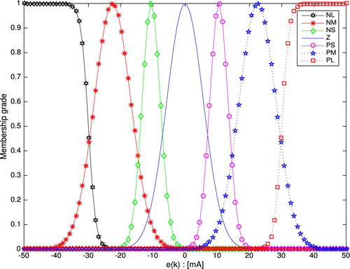
Figure 11. MiFRENc membership functions: experimental system.

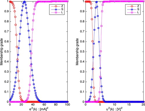
Table 3. Initial setting ${\beta }_{◻}(1)$: experimental system.

FRENa		MiFRENc
Parameter	Value	Parameter	Value
${\beta }_{\mathrm{NL}}(1)$	−3.25	${\beta }_{\mathrm{ZZ}}(1)$	0
${\beta }_{\mathrm{NM}}(1)$	−2.5	${\beta }_{\mathrm{ZS}}(1)$	0.1
${\beta }_{\mathrm{NS}}(1)$	−1.05	${\beta }_{\mathrm{ZL}}(1)$	0.2
${\beta }_{\mathrm{Z}}(1)$	0	${\beta }_{\mathrm{SZ}}(1)$	0.3
${\beta }_{\mathrm{PS}}(1)$	1.05	${\beta }_{\mathrm{SS}}(1)$	0.4
${\beta }_{\mathrm{PM}}(1)$	2.5	${\beta }_{\mathrm{SL}}(1)$	0.5
${\beta }_{\mathrm{PL}}(1)$	3.25	${\beta }_{\mathrm{LZ}}(1)$	0.6
		${\beta }_{\mathrm{LS}}(1)$	0.7
		${\beta }_{\mathrm{LL}}(1)$	0.8

Figure 12 displays the motor current $y(k)$ and the tracking error $e(k)$ to demonstrate the performance of the closed-loop system. The maximum absolute value of tracking error is $|e(k){|}_{\max }=48.2936$ (mA) and the average absolute value of tracking error at steady state is 0.4924 (mA) when $k=$1500–2000. Figure 13 shows the control effort $u(k)$. The estimated cost function $\hat{L}(k)$ is illustrated in Figure 14. 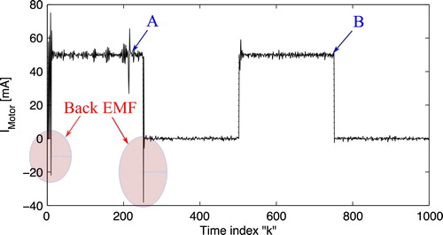The phase plane trajectory of $u(k)$ and $e(k)$ is plotted in Figure 15. Thus, the large variation is detected because of the back-EMF. In order to evaluate the proposed scheme working under the situation of back-EMF, the pulse-train trajectory is implemented with the response displayed in Figure 16. It is clear that the effect of back-EMF is eliminated within the second pulse (B).

Figure 12. Tracking performance $y(k)$ and $e(k)$: experimental system.

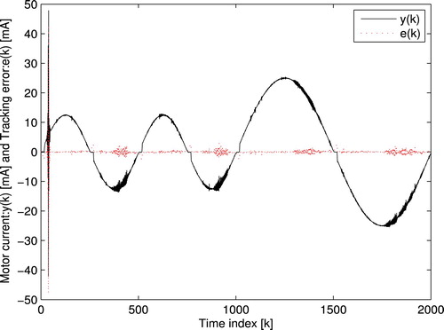
Figure 13. Control effort $u(k)$: experimental system.

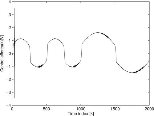
Figure 14. Estimated cost function $\hat{L}(k)$: experimental system.

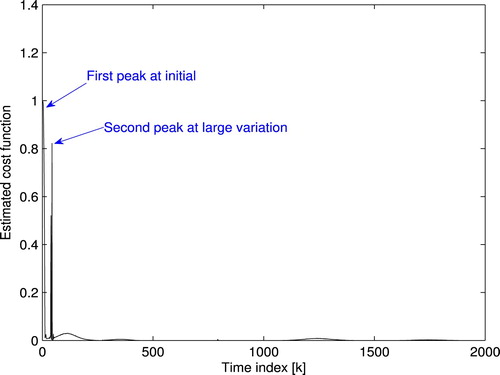
Figure 15. $u(k)$ and $e(k)$: experimental system.

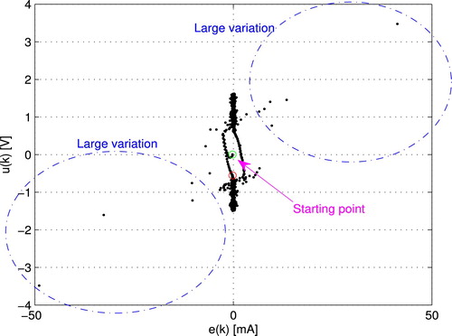
Figure 16. Pulse response: experimental system.

6. Conclusions

A model-free adaptive control for a class of non-affine discrete time systems has been developed by RL. The closed-loop system has been established by the output feedback with two adaptive networks FRENa and MiFRENc. The initial settings of FRENa and MiFRENc have been conducted according to the human knowledge of the controlled plant within the format of IF–THEN rules. The performance has been enchanted by the learning laws for both FRENa and MiFRENc while the tracking error and internal signals have been guaranteed the convergence over the reasonable compact sets. The numerical system and experimental results have represented to verify theoretical conjecture.

Disclosure statement

No potential conflict of interest was reported by the author(s).

Additional information

Funding

This work has been supported by Fundamental Research Funds for CINVESTAV-IPN and Mexican Research Organization CONACyT [grant number 257253].

Notes on contributors

C. Treesatayapun

C. Treesatayapun received the Ph.D. in elec- trical engineering from Chiang-Mai University, Thailand, in 2004. He was a production engineer at SAGA Elec- tronics (JRC-NJR) from 1998-2000 and was a head of electrical engineering program at North Chiang-Mai University, Thailand from 2001- 2007. He is currently a senior researcher at Department of robotic and advanced manufac- turing, Mexican Research Center and Advanced Technology, CINVESTAV-IPN, Saltillo campus, Mexico. His current research interests include automation and robotic system control and optimization, adaptive and learning algorithms and electric machine drives.

Appendix 1.

Proof of Theorem 4.1

Let us refer to the standard Lyapunov function as (A1) $\begin{array}{rl}V(k)& =V_1(k)+V_2(k)+V_3(k)+V_4(k)\\ & ={\rho }_1{e}^2(k)+\frac{{\rho }_2}{{\eta }_a}{\tilde{\beta }}_a^T(k){\tilde{\beta }}_a(k)+\frac{{\rho }_3}{{\eta }_c}{\tilde{\beta }}_c^T(k){\tilde{\beta }}_c(k)+{\rho }_4{\mathrm{\Lambda }}_c^2(k-1),\end{array}$(A1) where ${\rho }_1$, ${\rho }_2$, ${\rho }_3$ and ${\rho }_4$ are positive constants satisfying the following conditions: (A2) $\begin{array}{rl}& {\rho }_1>\frac{3}{4}p{\rho }_3,\end{array}$(A2) (A3) $\begin{array}{rl}& {\rho }_2>\frac{{\rho }_1{g}_M^2+({\rho }_3/8)q}{g_m}{\rho }_3,\end{array}$(A3) (A4) $\begin{array}{rl}& {\rho }_3>\frac{{\rho }_4}{{\delta }^2}\end{array}$(A4) and (A5) ${\rho }_4>\frac{{\rho }_3}{4}.$(A5) Utilising (14(14) $e(k+1)=g(k){\mathrm{\Lambda }}_a(k)+d_a(k).$(14) ), $\mathrm{\Delta }{V}_1(k)$ is obtained as (A6) $\begin{array}{rl}\mathrm{\Delta }{V}_1(k)& ={\rho }_1[e^2(k+1)-e^2(k)]\\ & ={\rho }_1[[g(k){\mathrm{\Lambda }}_a(k)+d_a(k){]}^2-e^2(k)]\\ & \le {\rho }_1[2g^2(k){\mathrm{\Lambda }}_a^2(k)+2d_a^2(k)-e^2(k)]\\ & \le -{\rho }_1{e}^2(k)+2{\rho }_1{g}_M^2{\mathrm{\Lambda }}_a^2(k)+2{\rho }_1{d}_{aM}^2.\end{array}$(A6) Recalling the tuning law in (26(26) $\begin{array}{rl}{\beta }_a(k+1)& ={\beta }_a(k)+{\eta }_a{e}_a(k)\sqrt{g(k)}{\varphi }_a(k)\\ & ={\beta }_a(k)+{\eta }_a[\sqrt{g(k)}{\mathrm{\Lambda }}_a(k)+\frac{1}{\sqrt{g(k)}}\hat{L}(k)]\sqrt{g(k)}{\varphi }_a(k)\\ & ={\beta }_a(k)+{\eta }_a[g(k){\mathrm{\Lambda }}_a(k)+\hat{L}(k)]{\varphi }_a(k).\end{array}$(26) ), $\mathrm{\Delta }{V}_2(k)$ is expressed as (A7) $\begin{array}{rl}\mathrm{\Delta }{V}_2(k)& =\frac{{\rho }_2}{{\eta }_a}[{\tilde{\beta }}_a^T(k+1){\tilde{\beta }}_a(k+1)-{\tilde{\beta }}_a^T(k){\tilde{\beta }}_a(k)]\\ & =-2{\rho }_2[g(k){\mathrm{\Lambda }}_a(k)+\hat{L}(k)]{\tilde{\beta }}_a^T(k)\varphi (k)+{\rho }_2{\eta }_a[g(k){\mathrm{\Lambda }}_a(k)\\ & +\hat{L}(k){]}^2{\varphi }_a^T(k)\varphi (k)\\ & =-2{\rho }_2{\mathrm{\Lambda }}_a(k)[g(k){\mathrm{\Lambda }}_a(k)]-2{\rho }_2{\mathrm{\Lambda }}_a(k)\hat{L}(k)\\ & +{\rho }_2{\eta }_a||{\varphi }_a(k)|{|}^2[g(k){\mathrm{\Lambda }}_a(k)+\hat{L}(k){]}^2.\end{array}$(A7) Applying the lower bound and upper bound of $g(k)$, it leads to (A8) $\begin{array}{rl}\mathrm{\Delta }{V}_2(k)& \le -2{\rho }_2{g}_m{\mathrm{\Lambda }}_a^2(k)-2{\rho }_2{\mathrm{\Lambda }}_a(k)\hat{L}(k)+{\rho }_2{\eta }_a||{\varphi }_a(k)|{|}^2{g}_M^2{\mathrm{\Lambda }}_a^2(k)\\ & +{\rho }_2{\eta }_a||{\varphi }_a(k)|{|}^2[{\hat{L}}^2(k)+2g(k){\mathrm{\Lambda }}_a(k)\hat{L}(k)]\\ & ={\rho }_2[-g_m{\mathrm{\Lambda }}_a^2(k)-(g_m-{\eta }_a||{\varphi }_a(k)|{|}^2{g}_M^2){\mathrm{\Lambda }}_a^2(k)\\ & -2{\mathrm{\Lambda }}_a(k)[I-{\eta }_a||{\varphi }_a(k)|{|}^{2}g(k)]\hat{L}(k)+{\eta }_a||{\varphi }_a(k)|{|}^2{\hat{L}}^2(k)]\\ & ={\rho }_2[-g_m{\mathrm{\Lambda }}_a^2(k)-(g_m-{\eta }_a||{\varphi }_a(k)|{|}^2{g}_M^2)[{\mathrm{\Lambda }}_a^2(k)\\ & +\frac{2{\mathrm{\Lambda }}_a(k)[I-{\eta }_a||{\varphi }_a(k)|{|}^{2}g(k)]\hat{L}(k)}{g_m-{\eta }_a||{\varphi }_a(k)|{|}^2{g}_M^2}]+{\eta }_a||{\varphi }_a(k)|{|}^2{\hat{L}}^2(k)]\\ & =-{\rho }_2{g}_m{\mathrm{\Lambda }}_a^2(k)-{\rho }_2(g_m-{\eta }_a||{\varphi }_a(k)|{|}^2{g}_M^2)||{\mathrm{\Lambda }}_a(k)\\ & +\frac{[1-{\eta }_a||{\varphi }_a(k)|{|}^{2}g(k)]\hat{L}(k)}{g_m-{\eta }_a||{\varphi }_a(k)|{|}^2{g}_M^2}|{|}^2\\ & +{\rho }_2\frac{1-{\eta }_a||{\varphi }_a(k)|{|}^2{g}_m}{g_m-{\eta }_a||{\varphi }_a(k)|{|}^2{g}_M^2}{\hat{L}}^2(k)\\ & \le -{\rho }_2{g}_m{\mathrm{\Lambda }}_a^2(k)+\frac{{\rho }_2}{g_m}{\hat{L}}^2(k)-{\rho }_2(g_m-{\eta }_a||{\varphi }_a(k)|{|}^2{g}_M^2)||{\mathrm{\Lambda }}_a(k)\\ & +\frac{[1-{\eta }_a||{\varphi }_a(k)|{|}^{2}g(k)]\hat{L}(k)}{g_m-{\eta }_a||{\varphi }_a(k)|{|}^2{g}_M^2}|{|}^2.\end{array}$(A8) By using the learning law of MiFRENc in (32(32) $\begin{array}{rl}{\beta }_c(k+1)& ={\beta }_c(k)-{\eta }_c{e}_c(k)\delta {\varphi }_c(k)\\ & ={\beta }_c(k)-{\eta }_c\delta [l(k)-\hat{L}(k-1)+\delta \hat{L}(k)]{\varphi }_c(k).\end{array}$(32) ), $\mathrm{\Delta }{V}_3(k)$ is derived as (A9) $\begin{array}{rl}\mathrm{\Delta }{V}_3(k)& =\frac{{\rho }_3}{{\eta }_c}[{\tilde{\beta }}_c^T(k+1){\tilde{\beta }}_c(k+1)-{\tilde{\beta }}_c^T(k){\tilde{\beta }}_c(k)]\\ & =\frac{{\rho }_3}{{\eta }_c}[-2{\eta }_c\delta e_c(k){\tilde{\beta }}_c^T(k){\varphi }_c(k)+{\eta }_c^2{\delta }^2{e}_c^2(k)||{\varphi }_c(k)|{|}^2]\\ & =-2{\rho }_3\delta {\mathrm{\Lambda }}_c(k)e_c(k)+{\rho }_3{\eta }_c{\delta }^2||{\varphi }_c(k)|{|}^2{e}_c^2(k).\end{array}$(A9) Recalling $e_c(k)$ in (28(28) $e_c(k)=\delta \hat{L}(k)-\hat{L}(k-1)+l(k),$(28) ) with $\pm \delta L(k)$ and $\pm L(k-1)$ and using (A10(A10) $\begin{array}{rl}{e}_c(k)& =\delta [\hat{L}(k)-L(k)]+\delta L(k)-[\hat{L}(k-1)-L(k-1)]-L(k-1)+l(k)\\ & =\delta [{\hat{\beta }}_c^T(k){\varphi }_c(k)-{\beta }_c^T{\varphi }_c(k)-{\epsilon }_c(k)]+\delta L(k)-L(k-1)+l(k)\\ & -[{\hat{\beta }}_c^T(k-1)F_c(k-1)-{\beta }_c^T{\varphi }_c(k-1)-{\epsilon }_c(k-1)]\\ & =\delta {\tilde{\beta }}_c^T(k){\varphi }_c(k)-{\tilde{\beta }}_c^T(k-1){\varphi }_c(k-1)+\delta L(k)-L(k-1)\\ & +l(k)-\delta {\epsilon }_c(k)+{\epsilon }_c(k-1)\\ & =\delta {\mathrm{\Lambda }}_c(k)-{\mathrm{\Lambda }}_c(k-1)+\delta L(k)-L(k-1)+l(k)-\delta {\epsilon }_c(k)\\ & +{\epsilon }_c(k-1)\end{array}$(A10) ), it yields (A10) $\begin{array}{rl}{e}_c(k)& =\delta [\hat{L}(k)-L(k)]+\delta L(k)-[\hat{L}(k-1)-L(k-1)]-L(k-1)+l(k)\\ & =\delta [{\hat{\beta }}_c^T(k){\varphi }_c(k)-{\beta }_c^T{\varphi }_c(k)-{\epsilon }_c(k)]+\delta L(k)-L(k-1)+l(k)\\ & -[{\hat{\beta }}_c^T(k-1)F_c(k-1)-{\beta }_c^T{\varphi }_c(k-1)-{\epsilon }_c(k-1)]\\ & =\delta {\tilde{\beta }}_c^T(k){\varphi }_c(k)-{\tilde{\beta }}_c^T(k-1){\varphi }_c(k-1)+\delta L(k)-L(k-1)\\ & +l(k)-\delta {\epsilon }_c(k)+{\epsilon }_c(k-1)\\ & =\delta {\mathrm{\Lambda }}_c(k)-{\mathrm{\Lambda }}_c(k-1)+\delta L(k)-L(k-1)+l(k)-\delta {\epsilon }_c(k)\\ & +{\epsilon }_c(k-1)\end{array}$(A10) or (A11) $\delta {\mathrm{\Lambda }}_c(k)=e_c(k)-\delta L(k)+{\mathrm{\Lambda }}_c(k-1)+L(k-1)-l(k)+\delta {\epsilon }_c(k)-{\epsilon }_c(k-1).$(A11) By using (A11(A11) $\delta {\mathrm{\Lambda }}_c(k)=e_c(k)-\delta L(k)+{\mathrm{\Lambda }}_c(k-1)+L(k-1)-l(k)+\delta {\epsilon }_c(k)-{\epsilon }_c(k-1).$(A11) ) and (16(16) $l(k)=p{e}^2(k)+q{u}^2(k),$(16) ), (A9(A9) $\begin{array}{rl}\mathrm{\Delta }{V}_3(k)& =\frac{{\rho }_3}{{\eta }_c}[{\tilde{\beta }}_c^T(k+1){\tilde{\beta }}_c(k+1)-{\tilde{\beta }}_c^T(k){\tilde{\beta }}_c(k)]\\ & =\frac{{\rho }_3}{{\eta }_c}[-2{\eta }_c\delta e_c(k){\tilde{\beta }}_c^T(k){\varphi }_c(k)+{\eta }_c^2{\delta }^2{e}_c^2(k)||{\varphi }_c(k)|{|}^2]\\ & =-2{\rho }_3\delta {\mathrm{\Lambda }}_c(k)e_c(k)+{\rho }_3{\eta }_c{\delta }^2||{\varphi }_c(k)|{|}^2{e}_c^2(k).\end{array}$(A9) ) can be derived as (A12) $\begin{array}{rl}\mathrm{\Delta }{V}_3(k)& =-2{\rho }_3{e}_c(k)[e_c(k)-\delta L(k)+{\mathrm{\Lambda }}_c(k-1)+L(k-1)-l(k)\\ & +\delta {\epsilon }_c(k)-{\epsilon }_c(k-1)]+{\rho }_3{\eta }_c{\delta }^2||{\varphi }_c(k)|{|}^2{e}_c^2(k)\\ & =-{\rho }_3[1-{\eta }_c{\delta }^2||{\varphi }_c(k)|{|}^2]e_c^2(k)-{\rho }_3{e}_c^2(k)+2{\rho }_3{e}_c(k)[\delta L(k)\\ & -{\mathrm{\Lambda }}_c(k-1)-L(k-1)+l(k)-\delta {\epsilon }_c(k)+{\epsilon }_c(k-1)]\\ & =-{\rho }_3[1-{\eta }_c{\delta }^2||{\varphi }_c(k)|{|}^2]e_c^2(k)-{\rho }_3{\delta }^2{\mathrm{\Lambda }}_c^2(k)+{\rho }_3[\delta L(k)\\ & -{\mathrm{\Lambda }}_c(k-1)-L(k-1)+l(k)-\delta {\epsilon }_c(k)+{\epsilon }_c(k-1){]}^2\\ & \le -{\rho }_3[1-{\eta }_c{\delta }^2||{\varphi }_c(k)|{|}^2]e_c^2(k)-{\rho }_3{\delta }^2{\mathrm{\Lambda }}_c^2(k)+\frac{{\rho }_3}{4}{\mathrm{\Lambda }}_c^2(k-1)\\ & +\frac{{\rho }_3}{4}{l}^2(k)+\frac{{\rho }_3}{4}[\delta L(k)-L(k-1){]}^2\\ & +\frac{{\rho }_3}{4}[\delta {\epsilon }_c(k)-{\epsilon }_c(k-1){]}^2\\ & \le -{\rho }_3[1-{\eta }_c{\delta }^2||F_c(k)|{|}^2]e_c^2(k)-{\rho }_3{\delta }^2{\mathrm{\Lambda }}_c^2(k)+\frac{{\rho }_3}{4}{\mathrm{\Lambda }}_c^2(k-1)\\ & +\frac{{\rho }_3}{4}p{e}^2(k)+\frac{{\rho }_3}{8}q{\mathrm{\Lambda }}_a^2(k)+\frac{{\rho }_3}{8}||{\beta }_a^T(k){\varphi }_a(k)|{|}^2\\ & +\frac{{\rho }_3}{4}[\delta L(k)-L(k-1){]}^2+{\rho }_3{\epsilon }_{cM}^2.\end{array}$(A12) Finally, $\mathrm{\Delta }{V}_4(k)$ is formulated as (A13) $\mathrm{\Delta }{V}_4(k)={\rho }_4[{\mathrm{\Lambda }}_c^2(k)-{\mathrm{\Lambda }}_c^2(k-1)].$(A13) Recalling (A6(A6) $\begin{array}{rl}\mathrm{\Delta }{V}_1(k)& ={\rho }_1[e^2(k+1)-e^2(k)]\\ & ={\rho }_1[[g(k){\mathrm{\Lambda }}_a(k)+d_a(k){]}^2-e^2(k)]\\ & \le {\rho }_1[2g^2(k){\mathrm{\Lambda }}_a^2(k)+2d_a^2(k)-e^2(k)]\\ & \le -{\rho }_1{e}^2(k)+2{\rho }_1{g}_M^2{\mathrm{\Lambda }}_a^2(k)+2{\rho }_1{d}_{aM}^2.\end{array}$(A6) ), (A8(A8) $\begin{array}{rl}\mathrm{\Delta }{V}_2(k)& \le -2{\rho }_2{g}_m{\mathrm{\Lambda }}_a^2(k)-2{\rho }_2{\mathrm{\Lambda }}_a(k)\hat{L}(k)+{\rho }_2{\eta }_a||{\varphi }_a(k)|{|}^2{g}_M^2{\mathrm{\Lambda }}_a^2(k)\\ & +{\rho }_2{\eta }_a||{\varphi }_a(k)|{|}^2[{\hat{L}}^2(k)+2g(k){\mathrm{\Lambda }}_a(k)\hat{L}(k)]\\ & ={\rho }_2[-g_m{\mathrm{\Lambda }}_a^2(k)-(g_m-{\eta }_a||{\varphi }_a(k)|{|}^2{g}_M^2){\mathrm{\Lambda }}_a^2(k)\\ & -2{\mathrm{\Lambda }}_a(k)[I-{\eta }_a||{\varphi }_a(k)|{|}^{2}g(k)]\hat{L}(k)+{\eta }_a||{\varphi }_a(k)|{|}^2{\hat{L}}^2(k)]\\ & ={\rho }_2[-g_m{\mathrm{\Lambda }}_a^2(k)-(g_m-{\eta }_a||{\varphi }_a(k)|{|}^2{g}_M^2)[{\mathrm{\Lambda }}_a^2(k)\\ & +\frac{2{\mathrm{\Lambda }}_a(k)[I-{\eta }_a||{\varphi }_a(k)|{|}^{2}g(k)]\hat{L}(k)}{g_m-{\eta }_a||{\varphi }_a(k)|{|}^2{g}_M^2}]+{\eta }_a||{\varphi }_a(k)|{|}^2{\hat{L}}^2(k)]\\ & =-{\rho }_2{g}_m{\mathrm{\Lambda }}_a^2(k)-{\rho }_2(g_m-{\eta }_a||{\varphi }_a(k)|{|}^2{g}_M^2)||{\mathrm{\Lambda }}_a(k)\\ & +\frac{[1-{\eta }_a||{\varphi }_a(k)|{|}^{2}g(k)]\hat{L}(k)}{g_m-{\eta }_a||{\varphi }_a(k)|{|}^2{g}_M^2}|{|}^2\\ & +{\rho }_2\frac{1-{\eta }_a||{\varphi }_a(k)|{|}^2{g}_m}{g_m-{\eta }_a||{\varphi }_a(k)|{|}^2{g}_M^2}{\hat{L}}^2(k)\\ & \le -{\rho }_2{g}_m{\mathrm{\Lambda }}_a^2(k)+\frac{{\rho }_2}{g_m}{\hat{L}}^2(k)-{\rho }_2(g_m-{\eta }_a||{\varphi }_a(k)|{|}^2{g}_M^2)||{\mathrm{\Lambda }}_a(k)\\ & +\frac{[1-{\eta }_a||{\varphi }_a(k)|{|}^{2}g(k)]\hat{L}(k)}{g_m-{\eta }_a||{\varphi }_a(k)|{|}^2{g}_M^2}|{|}^2.\end{array}$(A8) ), (A12(A12) $\begin{array}{rl}\mathrm{\Delta }{V}_3(k)& =-2{\rho }_3{e}_c(k)[e_c(k)-\delta L(k)+{\mathrm{\Lambda }}_c(k-1)+L(k-1)-l(k)\\ & +\delta {\epsilon }_c(k)-{\epsilon }_c(k-1)]+{\rho }_3{\eta }_c{\delta }^2||{\varphi }_c(k)|{|}^2{e}_c^2(k)\\ & =-{\rho }_3[1-{\eta }_c{\delta }^2||{\varphi }_c(k)|{|}^2]e_c^2(k)-{\rho }_3{e}_c^2(k)+2{\rho }_3{e}_c(k)[\delta L(k)\\ & -{\mathrm{\Lambda }}_c(k-1)-L(k-1)+l(k)-\delta {\epsilon }_c(k)+{\epsilon }_c(k-1)]\\ & =-{\rho }_3[1-{\eta }_c{\delta }^2||{\varphi }_c(k)|{|}^2]e_c^2(k)-{\rho }_3{\delta }^2{\mathrm{\Lambda }}_c^2(k)+{\rho }_3[\delta L(k)\\ & -{\mathrm{\Lambda }}_c(k-1)-L(k-1)+l(k)-\delta {\epsilon }_c(k)+{\epsilon }_c(k-1){]}^2\\ & \le -{\rho }_3[1-{\eta }_c{\delta }^2||{\varphi }_c(k)|{|}^2]e_c^2(k)-{\rho }_3{\delta }^2{\mathrm{\Lambda }}_c^2(k)+\frac{{\rho }_3}{4}{\mathrm{\Lambda }}_c^2(k-1)\\ & +\frac{{\rho }_3}{4}{l}^2(k)+\frac{{\rho }_3}{4}[\delta L(k)-L(k-1){]}^2\\ & +\frac{{\rho }_3}{4}[\delta {\epsilon }_c(k)-{\epsilon }_c(k-1){]}^2\\ & \le -{\rho }_3[1-{\eta }_c{\delta }^2||F_c(k)|{|}^2]e_c^2(k)-{\rho }_3{\delta }^2{\mathrm{\Lambda }}_c^2(k)+\frac{{\rho }_3}{4}{\mathrm{\Lambda }}_c^2(k-1)\\ & +\frac{{\rho }_3}{4}p{e}^2(k)+\frac{{\rho }_3}{8}q{\mathrm{\Lambda }}_a^2(k)+\frac{{\rho }_3}{8}||{\beta }_a^T(k){\varphi }_a(k)|{|}^2\\ & +\frac{{\rho }_3}{4}[\delta L(k)-L(k-1){]}^2+{\rho }_3{\epsilon }_{cM}^2.\end{array}$(A12) ) and (A13(A13) $\mathrm{\Delta }{V}_4(k)={\rho }_4[{\mathrm{\Lambda }}_c^2(k)-{\mathrm{\Lambda }}_c^2(k-1)].$(A13) ), $\mathrm{\Delta }V(k)$ is rewritten as (A14) $\begin{array}{rl}\mathrm{\Delta }V(k)& \le -\frac{{\rho }_1}{3}{e}^2(k)+{\rho }_1{g}_M^2{\mathrm{\Lambda }}_a^2(k)+{\rho }_1{d}_M^2\\ & -{\rho }_2{g}_m{\mathrm{\Lambda }}_a^2(k)-{\rho }_2(g_m-{\eta }_a||{\varphi }_a(k)|{|}^2{g}_M^2)||{\mathrm{\Lambda }}_a(k)+\\ & \frac{[1-{\eta }_a||{\varphi }_a(k)|{|}^{2}g(k)]L(k)}{g_m-{\eta }_a||{\varphi }_a(k)|{|}^2{g}_M^2}|{|}^2+\frac{{\rho }_2}{g_m}{L}^2(k)\\ & -{\rho }_3[1-{\eta }_c{\delta }^2||{\varphi }_c(k)|{|}^2]e_c^2(k)-{\rho }_3{\delta }^2{\mathrm{\Lambda }}_c^2(k)+\frac{{\rho }_3}{4}{\mathrm{\Lambda }}_c^2(k-1)\\ & +\frac{{\rho }_3}{4}p{e}^2(k)+\frac{{\rho }_3}{8}q{\mathrm{\Lambda }}_a^2(k)+\frac{{\rho }_3}{8}||{\beta }_a^T{\varphi }_a(k)|{|}^2\\ & +\frac{{\rho }_3}{4}[\delta L(k)-L(k-1){]}^2+{\rho }_3{\epsilon }_{cM}^2\\ & {\rho }_4[{\mathrm{\Lambda }}_c^2(k)-{\mathrm{\Lambda }}_c^2(k-1)]\\ & \le -[\frac{{\rho }_1}{3}-\frac{{\rho }_3}{4}p]e^2(k)-[{\rho }_2{g}_m-{\rho }_1{g}_M^2-\frac{{\rho }_3}{8}q]{\mathrm{\Lambda }}_a^2(k)\\ & -[{\rho }_3{\delta }^2-{\rho }_4]{\mathrm{\Lambda }}_c^2(k)-[{\rho }_4-\frac{{\rho }_3}{4}]{\mathrm{\Lambda }}_c^2(k-1)\\ & -{\rho }_3[1-{\eta }_c{\delta }^2||{\varphi }_c(k)|{|}^2]e_c^2(k)\\ & -{\rho }_2[g_m-{\eta }_a||{\varphi }_a(k)|{|}^2{g}_M^2]||{\mathrm{\Lambda }}_a(k)+\frac{[1-{\eta }_a||{\varphi }_a(k)|{|}^{2}g(k)]L(k)}{g_m-{\eta }_a||{\varphi }_a(k)|{|}^2{g}_M^2}|{|}^2\\ & +{\mathfrak{V}}_M\\ & \le -{\mathfrak{V}}_e{e}^2(k)-{\mathfrak{V}}_a{\mathrm{\Lambda }}_a^2(k)-{\mathfrak{V}}_{c0}{\mathrm{\Lambda }}_c^2(k)-{\mathfrak{V}}_{c1}{\mathrm{\Lambda }}_c^2(k-1)\\ & -{\mathfrak{V}}_c{e}_c^2(k)+{\mathfrak{V}}_M,\end{array}$(A14) where (A15) $\begin{array}{rl}{\mathfrak{V}}_M& \ge {\rho }_1{d}_m^2+{\rho }_3{\epsilon }_{cM}^2+\frac{{\rho }_3}{8}{\beta }_{aM}^2+[\frac{{\rho }_3}{8}(\gamma -1{)}^2+\frac{{\rho }_2}{g_o}]L_M^2\\ & -{\rho }_2[g_m-{\eta }_a||{\varphi }_a(k)|{|}^2{g}_M^2]||{\mathrm{\Lambda }}_a(k)\\ & +\frac{[1-{\eta }_a||{\varphi }_a(k)|{|}^{2}g(k)]L(k)}{g_m-{\eta }_a||{\varphi }_a(k)|{|}^2{g}_M^2}|{|}^2,\end{array}$(A15) (A16) $\begin{array}{rl}{\mathfrak{V}}_e& =\frac{{\rho }_1}{3}-\frac{{\rho }_3}{4}p,\end{array}$(A16) (A17) $\begin{array}{rl}{\mathfrak{V}}_a& ={\rho }_2{g}_m-{\rho }_1{g}_M^2-\frac{{\rho }_3}{8}q,\end{array}$(A17) (A18) $\begin{array}{rl}{\mathfrak{V}}_{c0}& ={\rho }_3{\delta }^2-{\rho }_4,\end{array}$(A18) (A19) $\begin{array}{rl}{\mathfrak{V}}_{c1}& ={\rho }_4-\frac{{\rho }_3}{4}\end{array}$(A19) and (A20) ${\mathfrak{V}}_c={\rho }_3[1-{\eta }_c{\delta }^2||{\varphi }_c(k)|{|}^2].$(A20) According to the conditions in (A2(A2) $\begin{array}{rl}& {\rho }_1>\frac{3}{4}p{\rho }_3,\end{array}$(A2) ) – (A5(A5) ${\rho }_4>\frac{{\rho }_3}{4}.$(A5) ), ${\mathfrak{V}}_e$, ${\mathfrak{V}}_a$, ${\mathfrak{V}}_{c0}$ and ${\mathfrak{V}}_{c1}$ are always positive. Furthermore, by setting the membership functions of FRENa and MiFRENc, the upper limits exist such that (A21) $0<||{\varphi }_a(k)|{|}^2\le {\nu }_a$(A21) and (A22) $0<||{\varphi }_c(k)|{|}^2\le {\nu }_c.$(A22) Combining with (34(34) $\begin{array}{rl}& 0<{\eta }_a\le \frac{g_m}{{\nu }_a{g}_M^2}\end{array}$(34) ) and (35(35) $0<{\eta }_c\le \frac{1}{{\nu }_c{\delta }^2},$(35) ), it leads to (A23) $g_m-{\eta }_a||{\varphi }_a(k)|{|}^2{g}_M^2>0$(A23) and (A24) ${\mathfrak{V}}_M\ge {\rho }_1{d}_m^2+{\rho }_3{\epsilon }_{cM}^2+\frac{{\rho }_3}{8}{\beta }_{aM}^2+[\frac{{\rho }_3}{8}(\gamma -1{)}^2+\frac{{\rho }_2}{g_o}]L_M^2.$(A24) By this mean, we have (A25) $\begin{array}{rl}& |e(k)|\ge {\mathrm{\Omega }}_e\doteq \sqrt{\frac{{\mathfrak{V}}_M}{{\mathfrak{V}}_e}},\end{array}$(A25) (A26) $\begin{array}{rl}& |{\mathrm{\Lambda }}_a(k)|\ge {\mathrm{\Omega }}_a\doteq \sqrt{\frac{{\mathfrak{V}}_M}{{\mathfrak{V}}_a}}\end{array}$(A26) and (A27) $|{\mathrm{\Lambda }}_c(k)|\ge {\mathrm{\Omega }}_c\doteq \sqrt{\frac{{\mathfrak{V}}_M}{{\mathfrak{V}}_{c0}}}.$(A27) The proof is completed here. $◻$

References

- Hou ZS, Wang Z. From model-based control to data-driven control: survey, classification and perspective. Inf Sci. 2013;235:3–35.
- Zhu Y, Hou ZS. Data-driven MFAC for a class of discrete-time nonlinear systems with RBFNN. IEEE Trans Neural Netw Learn Syst. 2014;25(5):1013–1020.
- Wang X, Li X, Wang J, et al. Data-driven model-free adaptive sliding mode control for the multi degree-of-freedom robotic exoskeleton. Inf Sci. 2016;327:246–257.
- Lin N, Chi R, Huang B. Data-driven recursive least squares methods for non-affined nonlinear discrete-time systems. Appl Math Modell. 2020;81:787–798.
- Kaldmae A, Kotta U. Input–output linearization of discrete-time systems by dynamic output feedback. Eur J Control. 2014;20:73–78.
- Treesatayapun C. Data input–output adaptive controller based on IF–THEN rules for a class of non-affine discrete-time systems: the robotic plant. J Intell Fuzzy Syst. 2015;28:661–668.
- Liu YJ, Tong S. Adaptive NN tracking control of uncertain nonlinear discrete-time systems with nonaffine dead-zone input. IEEE Trans Cybern. 2015;45(3):497–505.
- Zhang CL, Li JM. Adaptive iterative learning control of non-uniform trajectory tracking for strict feedback nonlinear time-varying systems with unknown control direction. Appl Math Model. 2015;39:2942–2950.
- Precup RE, Radac MB, Roman RC, et al. Model-free sliding mode control of nonlinear systems: algorithms and experiments. Inf Sci. 2017;381:176–192.
- Raj R, Mohan BM. Stability analysis of general Takagi–Sugeno fuzzy two-term controllers. Fuzzy Inf Eng. 2018;10(2):196–212.
- Zhang X, Zhang HG, Sun QY, et al. Adaptive dynamic programming-based optimal control of unknown nonaffine nonlinear discrete-time systems with proof of convergence. Neurocomputing. 2012;35:48–55.
- Eftekhari M, Zeinalkhani M. Extracting interpretable fuzzy models for nonlinear systems using gradient-based continuous ant colony optimization. Fuzzy Inf Eng. 2013;5(3):255–277.
- Liu D, Wang D, Yang X. An iterative adaptive dynamic programming algorithm for optimal control of unknown discrete-time nonlinear systems with constrained inputs. Inf Sci. 2013;220(20):331–342.
- Jiang H, Zhang H. Iterative ADP learning algorithms for discrete-time multi-player games. Artif Intell Rev. 2018;50(1):75–91.
- Liu D, Wang D, Zhao D, et al. Neural-network-based optimal control for a class of unknown discrete-time nonlinear systems using globalized dual heuristic programming. IEEE Trans Autom Sci Eng. 2012;9(3):628–634.
- Kiumarsi B, Lewis FL, Modares H, et al. Reinforcement Q-learning for optimal tracking control of linear discrete-time systems with unknown dynamics. Automatica. 2014;50(4):1167–1175.
- Yang Q, Jagannathan S. Reinforcement learning controller design for affine nonlinear discrete-time systems using online approximators. IEEE Trans Syst Man Cybern B Cybern. 2012;42(2):377–390.
- Ha M, Wang D, Liu D. Event-triggered constrained control with DHP implementation for nonaffine discrete-time systems. Inf Sci. 2020;519:110–123.
- Xu B, Yang C, Shi Z. Reinforcement learning output feedback NN control using deterministic learning technique. IEEE Trans Neural Netw Learn Syst. 2014;25(3):635–641.
- Liu YJ, Li S, Tong S, et al. Adaptive reinforcement learning control based on neural approximation for nonlinear discrete-time systems with unknown nonaffine dead-zone input. IEEE Trans Neural Netw Learn Syst. 2019;30(1):295–305.
- Allam E, Elbab HF, Hady MA, et al. Vibration control of active vehicle suspension system using fuzzy logic algorithm. Fuzzy Inf Eng. 2010;2(4):361–387.
- Niftiyev AA, Zeynalov CI, Poormanuchehri M. Fuzzy optimal control problem with non–linear functional. Fuzzy Inf Eng. 2011;3(3):311–320.
- Fei J, Wang T. Adaptive fuzzy-neural-network based on RBFNN control for active power filter. Int J Mach Learn Cybern. 2019;10:1139–1150.
- Treesatayapun C, Uatrongjit S. Adaptive controller with fuzzy rules emulated structure and its applications. Eng Appl Artif Intell. 2005;18:603–615.
- Treesatayapun C. Adaptive control based on IF–THEN rules for grasping force regulation with unknown contact mechanism. Robot Comput Integr Manuf. 2014;30:11–18.
- Abouheaf M, Gueaieb W. Neurofuzzy reinforcement learning control schemes for optimized dynamical performance. 2019 IEEE International Symposium on Robotic and Sensors Environments (ROSE). Ontario, Canada; 2019 June. p. 17–18.
- Treesatayapun C. Fuzzy-rule emulated networks based on reinforcement learning for nonlinear discrete-time controllers. ISA Trans. 2008;47:362–373.
- Wei Q, Lewis FL, Sun Q, et al. Discrete-time deterministic q-learning: a novel convergence analysis. IEEE Trans Cybern. 2017;47(5):1224–1237.