Scattered data approximation using radial basis function with a cubic polynomial reproduction for modelling leaf surface

ABSTRACT

Realistic leaf models are significant for numerous applications in the plant sciences, for instance, modelling pesticide droplet movement on the leaf surface. In this framework, a smooth surface is necessary to structure the foundation for a theoretical revision of a droplets motion on leaves. The radial basis function is convenient for scattered d-dimensional interpolation and usually extended by a polynomial P_k (x) of degree (k) to improve the method stability. In this research paper, we proposed a new technique for modelling a real leaf surface, which is based on enhancing a cubic polynomial term P₃ (x) to the multiquadric Radial basis function (CMRBF). The precision of the CMRBF method is confirmed by applying it to a virtual data and then to a real Frangipani and Anthurium data sets sampled using a laser scanner. It is concluded that the proposed CMRBF method produces a realistic and accurate representation of the leaf surface.

KEYWORDS:

• Interpolation
• virtual leaf
• radial basis function

SUBJECT CLASSIFICATION CODES:

• 93A30
• 65C20

1. Introduction

The primary aim of the research presented in this paper is the application of surface fitting methods to reconstruct the leaf image. This aim is important research topic because the precise leaf representation is necessitated for modelling virtual plant, modelling droplet spraying and spreading on the leaf surface and measured the amount of precipitation of pesticide or nutrients [1–3].

Even though the virtual plant modelling has been researched over the last decades. However, modelling of leaves has been deliberated recently by many researchers. Loch [4] used finite element method to model the surface of four types of leaves. Oqielat et al. [5,6] proposed a new hybrid method for modelling leaves surfaces based on joining the Clough-Tocher (CT) and radial basis function (RBF) methods. Moreover, Oqielat [7–9] reconstruct the surface of leaf using Hardy’s multiquadrics and Gaussion RBF interpolation. Furthermore, a comparison between surface fitting methods are also presented by Oqielat [10] and found that the hybrid multiquadric RBF-CT method is the best. Kempthorne et al. [11,12] reconstructed the surface of the cotton and wheat leaf using discrete smoothing -splines. In this paper, we added a cubic polynomial to the multiquadric RBF interpolant to reconstruct the leaf surface from three-dimensional (3D) real scattered points.

This research paper consists of five sections. An overview of the interpolation RBF and its shape parameter is presented in Section 2. In Section 3, the RBF approximation with a polynomial term is introduced. The global RBF that requires large memory and the compactly supported RBF (CS-RBF) that requires less memory and leads to faster computation also discussed here. Moreover, a numerical experiment to evaluate the accuracy of our method is given. In Section 4, Frangipani and Anthurium leaf surface is constructed using the CMRBF method. Finally, conclusion and future work are presented in Section 5.

2. RBFs method

RBFs approach was originally presented by Hardy [13] and it is an efficient method for resolving problems in engineering and sciences. RBFs are considered also for solving partial differential equations on irregular domains [14] and broadly employed across several fields resolving technical and non-technical problems. Introduction and reviews of the RBF theory can be found in Buhmann [15]. The approximation RBF to the function is given by(1) where , are the centres of the approximation RBF and are the coefficients of the RBF satisfies the system.(2) RBF offer’s many considerable advantages, e.g. the RBF interpolation is a smooth surface to approximate the function values at points and it can be applied for interpolation of scalar and vector fields. Moreover, it is applicable generally to d-dimensional problems. The computational complexity of a solution of the system given in Equation (2) is a system of size which has to be solved in order to compute the RBF coefficients and can become ill-conditioned with very small in magnitude singular values.

Examples of global RBFs are inverse multiquadric , inverse quadratic, Gaussian RBF, thin plate splines and the Hardy’s multiquadric [13], which is considered in this paper. The shape parameter is defined behaviour of RBF and has an impact on the accuracy of RBF interpolate. For example, for some values of the problem may become ill-conditioned. Hardy [13] suggested a value of where is the distance between a data point and its closest neighbour. Rippa [16] proposed and algorithm for the choice of best value for that minimizes the cost function and he showed that the value of has a great impact on the approximation quality of the RBF. Scheuerer [17] presented a refinement algorithm of Rippa’s algorithm based on the Euclidean norm. Gregory [18] studied an extension of the Rippa method that can be applied for the solution of PDF of RBF pseudo-spectral methods. Majdisova [19] proposed RBF interpolation approach of large data points that uses a data structure for a spare matrix where the shape parameter was determined experimentally.

3. RBF approximation with a polynomial reproduction

In this research article, we describe the manipulation of meshless representation. The meshless technique is based on the scheme of RBF and leads to a solution of a linear system of equations. The RBFs are separated into two parts: the CS-RBF and the global RBF. Using CS-RBF to fit scattered data requires less memory and leads to faster computation of the linear system because A is a sparse matrix. Many RBFs and their properties have been extensively examined in [19–21].

The RBF is convenient for scattered -dimensional interpolation and usually extended by a polynomial of degree () to improve the stability of the method. In this paper, we used a polynomial of degree three, i.e. k = 3, which is given by(3) where . For a given data points and the associated function values to be interpolated, we obtain the interpolation function that satisfies:(4) where is the multiquadric RBF, is the distance between the interpolation point and the rest of the data points , , is the number of nodes, is the polynomial in the coordinates space , is the number of basis function for the polynomial, and are the interpolation coefficients. Formula (4) after substitution becomes:(5) and for conditionally positive definite RBF’s, additional condition is applied. The coefficients and in formula (5) can be evaluated by enforcing the formula to be satisfied at the N data points about a point . Now, formula (5) can be displayed in a linear system of the form , where: For -dimensional case, we want to solve a linear system of equation of size , where N is the number of data points and k is the polynomial degree. In the case of local RBF, the matrix M will be spare and calculation needed can be decreased while in the global case the matrix M will be full rank. The truncated singular value decomposition of is applied to solve the system .

3.1. Numerical experiment for the Franke data

In this section, we exhibit the outcomes of the numerical investigation for the proposed mathematical technique (CMRBF) given in Section 3. Two sets of data points (consists of 100 points and 33 points) and six test functions taken from [22] are applied here either globally or locally to evaluate the accuracy of our CMRBF method using the root mean square error (RMS) given in Equation (5):(6) where are the interpolation CMRBF values at the data points () and are the given function values at the same data points.

The global MRBF with a cubic polynomial interpolant (global CMRBF) is built from the points and then we used it to approximate the 33 surface values. While the local MRBF with a cubic polynomial interpolant (local CMRBF) is built for each point () of the 33 points from the nearest 20 points (), then the local CMRBF are used to estimate the surface value for that specific point (). In both cases, we used Rippa algorithm [16] to estimate the MRBF shape parameter globally using the points.

3.1.1 Results and discussion

The RMS errors acquired for the global and local MRBF with a cubic polynomial for the six test functions is given in Table 1. The parameter α in both methods is calculated using Rippa algorithm [16]. The observations from Table 1 show that employing the local MRBF with a cubic polynomial produces less accurate RMS than using global MRBF with a cubic polynomial except for the function F2 the RMS is slightly better. Moreover, using local MRBF with a cubic polynomial is computationally costly than using global MRBF with a cubic polynomial because a dense matrix of size 20 × 20 (see Equation (2)) demands to be resolved at each time we apply the local method. Notice that the value of the parameter (c) is variant between 0.1 and 2.5 depending on the used function, and this is an evidence that this parameter has a big influence on the quality of the RBF approximation, i.e. RMS error. In conclusion, employing global MRBF with a cubic polynomial produces more accurate RMS error than using the local MRBF with a cubic polynomial. Therefore, we bring this conclusion to the next section and investigate the suitability of the global MRBF with a cubic polynomial method (CMRBF) for a real leaf data set.

Table 1. A comparison of the RMS error using the global and the local MRBF with a cubic polynomial.

Function	C	With a cubic polynomial
		Global MRBF	Local MRBF
F1	0.1842	3.1e–003	5.0e–003
F2	0.0634	4.8e–003	4.4e–003
F3	0.5370	2.5e–004	4.0e–004
F4	0.8527	1.6e–005	1.4e–004
F5	0.5593	2.6e–004	2.4e–003
F6	1.0563	5.0e–005	7.4e–005

4. Application of the CMRBF technique to a real leaf data set

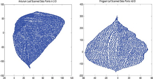
In this section, we applied the proposed multiquadric Radial basis function with a cubic polynomial (CMRBF) method to model a real Anthurium and Frangipani leaf data given in Figure 1. Preprocessing steps are required to employ the CMRBF method. These steps are, firstly, point selection from the whole data set. A digitizing device called a laser scanner is used by Loch [4] to collect the Anthurium and Frangipani leaf data points, where it is enough to sample the exterior points of the leaf to be able to capture the leaf surface. The collected surface points for Anthurium leaf were 4688 and 79 boundary points and for the Frangipani leaf, they were 3388 and 17 boundary points. The boundary points, see Figure 3, were chosen from the leaf points by hand using a software called Point Picker by [23]. Secondly, a new reference plane for the collected leaf data is important because the chance of vertical surfaces and multivalued of the data points returned by the scanner. Finally, the choice of the parameter for the RBF is important to obtain more accurate leaf surface. Therefore, in this research we adapted Rippa method [16] to compute the RBF parameter.

Figure 1. The 4688 scanned points for the Anthurium leaf (left figure) and the 3388 scanned points for the Frangipani leaf (right figure) in 2D.

4.1 Leaf reference plane

To model the leaf surface using the proposed CMRBF method, a new reference plane for the data are necessary for many reasons. Firstly, there is a possibility for measurement error in the coordinates system. Secondly, the plane of the leaf data scanned points may not necessarily correspond with the xy-plane (see Figure 2). Finally, for the chance of vertical surfaces and multivalued of the data points returned by the scanner, see Oqielat [5].

Figure 2. The Anthurium leaf data before projection into a new reference plane (left figure) and after projection (right figure).

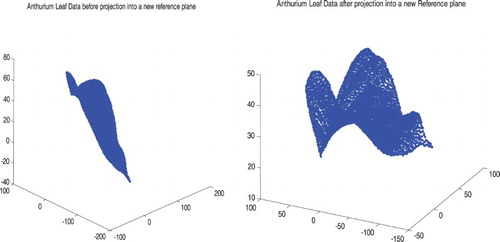
There are different kinds of best fit planes. In this paper, an orthogonal distance regression plane fit to the leaf data points is applied as reference plane and then we rotate the coordinate system to get the new reference plane as -plane, see Figure 2. Finding the orthogonal distance regression plane is an eigenvector problem. It is quite involved; the best solution uses the singular value decomposition.

Given data points , we want to fit these data using the orthogonal distance regression plane:(7) starting with the distance from a point to a plane, we want to find a, b and d that minimize to achieve the best fit as follows. Set the partial derivative with respect to to be zero,(8) (9) where is the centroid of the data and it lies in the plane. By substitutes into Equation (7) of the plane we obtain:(10) rewrite as . Then the matrix representation of last equation is defined aswhere and is called Rayleigh quotient and it is minimized by the eigenvector of (A) that corresponds to its smallest eigenvalue. The eigenvalues of A are the squares of the singular values of M, and the eigenvectors of A are the singular vectors of M. In conclusion, the orthogonal least squares 3D plane contains the centroid of the data, and its normal vector is the singular vector of M corresponding to its smallest singular value. The data points after they are projected to the new reference plane (see Figure 2) are given bywhere represents the rotation matrix that rotates the unit normal vector of the orthogonal distance regression plane about the x-axis and y-axis, for more details see [5]. Finally, after we projected the leaf data points into the new reference plane, The CMRBF interpolation method is then employed to model (reconstruct) the surface of the Anthurium and Frangipani leaf shown in Figure 1.

4.2 Numerical experiments for the leaf surface

The results of employing our proposed technique (CMRBF) to the Anthurium and Frangipani leaf data points shown in Figure 1 are given in Table 2. For the Anthurium leaf, one global CMRBF is constructed from 212 points (a subset of the 4767 leaf data points), while for the Frangipani leaf, the global CMRBF is built from 141 points (a subset of the 3405 leaf data points), see Figure 3. The rest of the leaf data points (4555 points for Anthurium leaf and 3264 points for Frangipani) is then used to assess the quality of the approximation of the CMRBF method. The RMS (given in Equation (6)) and the maximum error associated with the surface fit in relation to the maximum variation in z given in Equation (11) were used to measure the error:(11) where are the interpolant CMRBF values at the data points () and are the given function values at the same data points.

Figure 3. The 212 points that used to construct a global MRBF for the Anthurium leaf (left figure). The figure on the right represents the 141 points that used to construct a global MRBF for the Frangipani leaf.

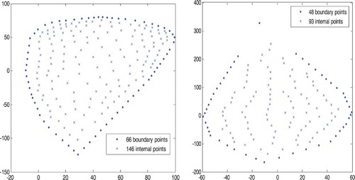
Table 2. The relative RMS and relative maximum error for the Anthurium and Frangipani leaf data points computed using the global MRBF with a cubic polynomial.

	Global MRBF With a cubic polynomial
	Anthurium leaf	Frangipani leaf
Maximum error	4.7e00–2	9.9e–002
Relative RMS	7.8e00–3	1.7e–002
Number of points tested	4555	3264
Number of boundary points	79	17
The RBF shape parameter (c)	0.5	0.1

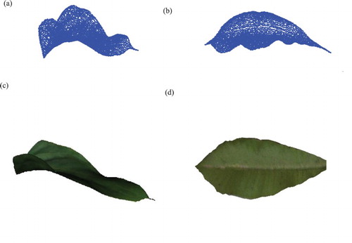
Table 2 shows the scaled maximum errors (Equation (11)) and the relative RMS (Equation (6)) for the Anthurium and Frangipani leaf data, respectively, using the global CMRBF method. The global RBF is developed from 212 points for Anthurium leaf and 141 points for the Frangipani leaf. A total of 4555 and 3264 data points were used to evaluate the accuracy of the two methods. The optimal value of the multiquadric RBF is computed using Rippa algorithm for both leaves and it was 0.5 for the Anthurium leaf and 0.1 for the Frangipani leaf. One observes from Table 2 that the relative RMS produced using CMRBF is better than the maximum error. Moreover, our proposed CMRBF method creates an accurate representation of the leaf surface (see Figure 4) and this confirms our outcomes for Franke data set [22] given in Section 3.

Figure 4. (a) and (b) represent the Anthurium and Frangipani leaf surface model, respectively, constructed from the points (shown in Figure 2) using the proposed CMRBF method. (c) and (d) the corresponding visualization of the Anthurium and Frangipani leaf model.

5. Results and conclusion

A surface fitting method that combines a cubic polynomial with multiquadric RBF (CMRBF) to model the leaf surface from 3D scanned data set is introduced in this research. The CMRBF is applied to reconstruct the surface of two types of leaves and we concluded that the algorithm offered an accurate representation for the leaf surface (see Figure 4). The leaf model can be used for modelling a droplet of water [24–29] or pesticide movement, spraying and spreading on a leaf surface.

Acknowledgements

The author thanks the reviewer for the perceptive comments on the manuscript that developed the final appearance of the paper.

Disclosure statement

No potential conflict of interest was reported by the author.

References

- Dorr G, Kempthorne D, Mayo L, et al. Towards a model of spray–canopy interactions: interception, shatter, bounce and retention of droplets on horizontal leaves. Ecol Model. 2014;290:94–101. doi: 10.1016/j.ecolmodel.2013.11.002
- Lisa C, McCue S, Moroney T, et al. Simulating droplet motion on virtual leaf surfaces. R Soc Open Sci. 2016;2: 1–17.
- Oqielat M, Turner I, Belward J, et al. Modelling water droplet movements on a leaf surface. Math Comput Simulat. 2011;81:1553–1571. doi: 10.1016/j.matcom.2010.09.003
- Loch B. Surface fitting for the modelling of plant leaves [Ph.D. thesis]. Brisbane: University of Queensland; 2004.
- Oqielat M, Turner I, Belward J. A hybrid Clough-Tocher method for surface fitting with application to leaf data. Appl Math Model. 2009;33:2582–2595. doi: 10.1016/j.apm.2008.07.023
- Oqielat MN, Belward JA, Turner IW, et al. A hybrid Clough–Tocher radial basis function method for modelling leaf surfaces. In: Oxley L, Kulasiri D, editors. MODSIM 2007: International Congress on Modelling and Simulation, December 2007. Model Simu Soc Aust New; 2007. p. 400–406.
- Oqielat M. Surface fitting methods for modelling leaf surface from scanned data. J King Saud Univ – Sci. Forthcoming.
- Oqielat M, Ogilat O, Al-Oushoush N, et al. Radial basis function method for modelling leaf surface from real leaf data. Aust J Basic Appl Sci. 2017;11(13):103–111.
- Oqiela M, Ogilat O. Application of Gaussion radial basis function with cubic polynomial for modelling leaf surface. J Math Anal. 2018;9(2):78–87.
- Oqielat M. Comparison of surface fitting methods for modelling leaf surfaces. Ital J Pure Appl Math. Forthcoming.
- Kempthorne D, Turner I, Belward J, et al. Surface reconstruction of wheat leaf morphology from three-dimensional scanned data. Funct Plant Biol. 2015;42:444–451. doi: 10.1071/FP14058
- Kempthorne D, Turner I, Belward J. A comparison of techniques for the reconstruction of leaf surfaces from scanned data. SIAM J Sci Comput. 2014;36(6):B969–B988. doi: 10.1137/130938761
- Hardy R. Theory and applications of the multiquadric-biharmonic method 20 years of discovery 1968–1988. Comput Math Appl. 1990;19:163–208. doi: 10.1016/0898-1221(90)90272-L
- Hon Y, Sarler B, Yun D. Local radial basis function collocation method for solving thermo-driven fluid-flow problems with free surface. Eng Anal Bound Elem. 2015;57:2–8. doi: 10.1016/j.enganabound.2014.11.006
- Buhmann M. Radial basis functions: theory and implementations. New York: Cambridge University Press; 2003.
- Rippa S. An algorithm for selecting a good value for the parameter c in radial basis function interpolation. Adv Comput Math. 1999;11:193–210. doi: 10.1023/A:1018975909870
- Scheuerer M. An alternative procedure for selecting a good value for the parameter c in RBF-interpolation. Adv Comput Math. 2011;34(1):105–126. doi: 10.1007/s10444-010-9146-3
- Gregory E, Fasshauer G, Zhang J. On choosing optimal shape parameters for RBF approximation. Numer Algorithms. 2007;45(1–4):345–368. doi: 10.1007/s11075-007-9072-8
- Majdisova Z, Skala V. Radial basis function approximations: comparison and applications. Appl Math Model. 2017;51:728–743. doi: 10.1016/j.apm.2017.07.033
- Skala V. RBF interpolation with CSRBF of large data sets. Int Conference Comp Sci. 2017;12–14.
- Turner I, Belward J, Oqielat M. Error bounds for least square gradient estimates. SIAM J Sci Comput. 2008;32(4):2146–2166. doi: 10.1137/080744906
- Franke R. Scattered data interpolation: tests of some methods. Math Comput. 1982;38:181–200.
- Hanan J, Loch B, McAleer T. Processing laser scanner plant data to extract structural information. Brisbane: Advanced Computational Modelling Centre, University of Queensland; 2007.
- Sheikholeslami M, Shehzad S. Simulation of water based nanofluid convective flow inside a porous enclosure via non-equilibrium model. Int J Heat Mass Transfer. 2018;120:200–1212.
- Sheikholeslami M, Seyednezhad M. Simulation of nanofluid flow and natural convection in a porous media under the influence of electric field using CVFE. Int J Heat Mass Transfer. 2018;120:772–781. doi: 10.1016/j.ijheatmasstransfer.2017.12.087
- Sheikholeslami M, Rokni H. CVFEM for effect of Lorentz forces on nanofluid flow in a porous complex shaped enclosure by means of non-equilibrium model. J Mol Liq. 2018;254:446–462. doi: 10.1016/j.molliq.2018.01.130
- Sheikholeslami M. Numerical investigation for CuO-H2O nanofluid flow in a porous channel with magnetic field using mesoscopic method. J Mol Liq. 2018;249:739–746. doi: 10.1016/j.molliq.2017.11.069
- Sheikholeslami M. CuO-water nanofluid flow due to magnetic field inside a porous media considering Brownian motion. J Mol Liq. 2018;249:921–929. doi: 10.1016/j.molliq.2017.11.118
- Sheikholeslami M. Numerical investigation of nanofluid free convection under the influence of electric field in a porous enclosure. J Mol Liq. 2018;249:1212–1221. doi: 10.1016/j.molliq.2017.11.141