A numerical technique for solving multi-dimensional fractional optimal control problems

ABSTRACT

In this article, we use the operation matrix (OM) of Riemann–Liouville fractional integral of the shifted Gegenbauer polynomials with the Lagrange multiplier method to provide efficient numerical solutions to the multi-dimensional fractional optimal control problems. The proposed technique transforms the under consideration problems into sets of nonlinear equations which are easy to solve. Numerical tests including numerical comparisons with some existing methods are introduced to demonstrate the accuracy and efficiency of the suggested technique.

KEYWORDS:

• Riemann–Liouville fractional integral operator
• fractional optimal control problems
• operational matrix
• shifted Gegenbauer polynomials
• Lagrange multiplier method

1. Introduction

The mathematical topic of optimal control problems (OCPs) has received much attentions in the last years because it has a lot of important applications in physics, chemistry, engineering, etc. [1, 2]. Recently, fractional calculus has demonstrated its accuracy in modelling many applications in various scientific fields [3–5]

Fractional optimal control problem (FOCP) is an OCP in which the differential equations governing the dynamics of the system contain at least one fractional derivative operator. Due to the various applications of FOCPs in physics and engineering, they received much attentions from many researchers. these applications include the materials with memory and hereditary effects, dynamical processes containing gas diffusion and heat conduction in fractal porous media. Other applications of FOCPs are given in [1, 6]. Because of a lot of FOCPs does not have analytical exact solutions, numerous numerical methods are offered to overcome these problems [7–12]. In recent years, various OMs for different polynomials like Chebyshev polynomials [13, 14], Legendre polynomials [11, 15], Jacobi polynomials [10, 16, 17], Bernstein polynomials [18] and Lagguerre polynomial [19] have been developed to cover the numerical solutions of different types of fractional differential equations [20–23]. Our technique depends on the OM of RL fractional integral of shifted Gegenbauer polynomial (SGPs). The Gegenbauer polynomials have many useful properties. They generalize Legendre polynomials $L_j\left(t\right)$ and Chebyshev polynomials of the first $T_j\left(t\right)$ and second $U_j\left(t\right)$ kind, and they are special cases of Jacobi polynomials. The most important characteristic of SGPs is achieving rapid rates of convergence [24–27]. This encourages us to use these polynomials in the suggested technique as basis functions for finding the approximate solutions to a wide class of FOCPs in the following form: (1) $\mathrm{Min}.J={\int }_0^{t}f(t,x_j(t),u(t\left)\right)\mathrm{d}t,$(1) subject to (2) $D^{\left(\nu \right)}{x}_j\left(t\right)=g_j(t,x_j(t\left)\right)+b_j\left(t\right)u\left(t\right),$(2) with $D^{\left(i\right)}{x}_j\left(0\right)=x_j^{\left(i\right)}\left(0\right),i=0,1,\dots ,m-1,j=1,2,\dots ,n,$ where $D^{\left(\nu \right)}$ is the Caputo fractional derivative of order $\nu ,m-1<\nu \le m$ and $b_j\left(t\right)\ne 0,n$ is the number of variables. In the proposed technique; the state and the control variables are approximated by SGPs. By using the OM of Riemann–Liouville fractional integral (RLFI) of the SGPs with the Lagrange multiplier method (LMM), the FOCPs are reduced to simple sets of nonlinear equations (NEs). The efficiency of the proposed technique is demonstrated by some numerical examples including problems in one-, two- and three-dimensional spaces, Also numerical comparisons between the suggested technique and some published results are held.

The rest of the paper is systemized as follows: We begin with some preliminaries of fractional calculus and GPs. In Section 3, the shifted Gegenbauer operational matrix (SGOM) of RL fractional integral is derived. In Section 4, the convergence of the proposed method is discussed. In Section 5, the proposed technique of applying SGOM of fractional integration for solving FOCPs is presented. In Section 6, some illustrative examples are offered. Finally concluding remarks end the paper.

2. Preliminaries and definitions

2.1. Fractional calculus definitions

Definition 2.1

One of the popular definitions of the fractional integral is the Riemann–Liouville (RL), which get from the relation (3) $\begin{array}{r}\begin{array}{rl}{I}^{\nu }f\left(t\right)& =\frac{1}{\mathrm{\Gamma }\left(\nu \right)}{\int }_0^t(t-\xi {)}^{\nu -1}f(\xi )\mathrm{d}\xi ,\\ & m-1<\nu <m,m\in N,\nu >0,t>0,\\ I^{0}f\left(t\right)& =f\left(t\right).\end{array}\end{array}$(3) The operator $I^{\nu }$ has properties said in [28], we just recall the next property (4) $I^{\nu }{t}^{\beta }=\frac{\mathrm{\Gamma }(\beta +1)}{\mathrm{\Gamma }(\nu +\beta +1)}{t}^{\nu +\beta }.$(4)

Definition 2.2

$D^{\nu }$ is the RL fractional derivative of order ν is defined by (5) $\begin{array}{rl}{D}^{\nu }f\left(t\right)& =\frac{{\mathrm{d}}^m}{\mathrm{d}{x}^m}\left(I^{m-\nu }f\right(t\left)\right),\\ & m-1<\nu \le m,m\in N,\nu \in R,\end{array}$(5) where m is the smallest integer greater than ν.

Lemma 2.1

If $m-1<\nu \le m,m\in N,$ then (6) $\begin{array}{rl}& D^{\nu }{I}^{\nu }f\left(t\right)=f\left(t\right),\\ & I^{\nu }{D}^{\nu }f\left(t\right)=f\left(t\right)-\sum _{i=0}^{m-1}{f}^{\left(i\right)}\left(0^{+}\right)\frac{t^i}{i!},t>0.\end{array}$(6)

2.2. Shifted Gegenbauer polynomials and their properties

The shifted ultraspherical (Gegenbauer) polynomials $C_{S,j}^{\left(\alpha \right)}\left(t\right),$ of degree $j\in {\mathbb{Z}}^{+},$ with the associated parameter $\alpha >\frac{-1}{2}$ are a sequence of real polynomials in the finite domain $[0,L].$ They are a family of orthogonal polynomials which has many properties:

The analytical form of the SGP is given by (7) $\begin{array}{rl}{C}_{S,j}^{\left(\alpha \right)}\left(t\right)& =\sum _{k=0}^j(-1{)}^{j-k}\frac{\mathrm{\Gamma }(\alpha +\frac{1}{2})\mathrm{\Gamma }(j+k+2\alpha )}{\mathrm{\Gamma }(k+\alpha +\frac{1}{2})\mathrm{\Gamma }\left(2\alpha \right)(j-k)!k!L^k}{t}^k,\\ C_{S,j}^{\left(\alpha \right)}\left(0\right)& =(-1{)}^j\frac{\mathrm{\Gamma }(j+2\alpha )}{\mathrm{\Gamma }\left(2\alpha \right)j!}\end{array}$(7) and $\begin{array}{rl}{C}_{S,j}^{\left(\alpha \right)}\left(t\right)& =C_j^{\left(\alpha \right)}\left(\frac{2t}{L}-1\right),C_{S,0}^{\left(\alpha \right)}\left(t\right)=1,\\ C_{S,1}^{\left(\alpha \right)}\left(t\right)& =\frac{2t}{L}-1.\end{array}$

The orthogonal relation of SGPs is: (8) $\begin{array}{rl}⟨C_{S,i}^{\left(\alpha \right)}\left(t\right),C_{S,j}^{\left(\alpha \right)}\left(t\right)⟩& ={\int }_0^L{C}_{S,i}^{\left(\alpha \right)}\left(t\right)C_{S,j}^{\left(\alpha \right)}\left(t\right){\omega }_S^{\left(\alpha \right)}\left(t\right)\mathrm{d}t\\ & ={\lambda }_{S,j}^{\left(\alpha \right)}{\delta }_{i,j},\end{array}$(8) where ${\omega }_S^{\left(\alpha \right)}\left(t\right)$ is the weight function, and it is even function given from the relation ${\omega }_S^{\left(\alpha \right)}\left(t\right)=(tL-t^2{)}^{\alpha -1/2}$ and ${\lambda }_{S,j}^{\left(\alpha \right)}={\left(\frac{L}{2}\right)}^{2\alpha }{\lambda }_j^{\left(\alpha \right)}.$

This polynomial recover the shifted Chebyshev polynomial of the first kind $T_{S,j}\left(t\right)\equiv C_{S,j}^{\left(0\right)}\left(t\right),$ the shifted Legendre polynomial $L_{S,j}\left(t\right)\equiv C_{S,j}^{\left(1/2\right)}\left(t\right),$ and the shifted Chebyshev polynomial of the second kind $C_{S,j}^{\left(1\right)}\left(t\right)\equiv \left(1/\right(j+1\left)\right)U_{S,j}\left(t\right)$.

The square integrable function $y\left(t\right)$ in $[0,L]$ is approximated by SGPs as: $y\left(t\right)=\sum _{j=0}^N{\tilde{y}}_j{C}_{S,j}^{\left(\alpha \right)}\left(t\right),$ where the coefficients ${\tilde{y}}_j$ are getting from (9) ${\tilde{y}}_j=\left({\lambda }_{S,j}^{\left(\alpha \right)}{)}^{-1}{\int }_0^{L}y\right(t\left){\omega }_S^{\left(\alpha \right)}\right(t\left)C_{S,j}^{\left(\alpha \right)}\right(t)\mathrm{d}t.$(9) The approximation of function $y\left(t\right)$ in the vector form is defined by (10) $y\left(t\right)=Y^T\phi \left(t\right),$(10) where $Y^T=[{\tilde{y}}_0,{\tilde{y}}_1,\dots ,{\tilde{y}}_N]$ is the shifted Gegenbauer coefficient vector, and (11) $\phi \left(t\right)=\left[C_{S,0}^{\left(\alpha \right)}\right(t),C_{S,1}^{\left(\alpha \right)}(t),\dots ,C_{S,N}^{\left(\alpha \right)}(t){]}^T$(11) is the shifted Gegenbauer vector. The q times repeated integration of Gegenbauer vector is (12) $I^q\phi \left(t\right)\simeq P^{\left(q\right)}\phi \left(t\right),$(12) where $P^{\left(q\right)}$ is called the OM of the integration of $\phi \left(t\right)$.

3. Fractional SGOM of integration

In this section, the SGOM of RLFI will be derived.

Theorem 3.1

Let $\phi \left(t\right)$ be the shifted Gegenbauer vector and $\nu >0$ then (13) $I^{\nu }\phi \left(t\right)\simeq P^{\left(\nu \right)}\phi \left(t\right),$(13) where $t\in [0,1]$ and $P^{\left(\nu \right)}$ is called OMFI of order ν in the RL sense, it is an $(N+1)\times (N+1)$ and is written as (14) $P^{\left(\nu \right)}=\left(\begin{array}{cccc}\sum _{k=0}^0{\xi }_{0,0,k}& \sum _{k=0}^0{\xi }_{0,1,k}& \cdots & \sum _{k=0}^0{\xi }_{0,N,k}\\ \sum _{k=0}^1{\xi }_{1,0,k}& \sum _{k=0}^1{\xi }_{1,1,k}& \cdots & \sum _{k=0}^1{\xi }_{1,N,k}\\ ⋮& ⋮& \cdots & ⋮\\ \sum _{k=0}^i{\xi }_{i,0,k}& \sum _{k=0}^i{\xi }_{i,1,k}& \cdots & \sum _{k=0}^i{\xi }_{i,N,k}\\ ⋮& ⋮& \cdots & ⋮\\ \sum _{k=0}^N{\xi }_{N,0,k}& \sum _{k=0}^N{\xi }_{N,1,k}& \cdots & \sum _{k=0}^N{\xi }_{N,N,k}\end{array}\right),$(14) where ${\xi }_{i,j,k}$ is given by ${\xi }_{i,j,k}=\mathrm{\Xi }\times \mathrm{{\rm Y}},$ where (15) $\begin{array}{rl}\mathrm{\Xi }& =\sum _{k=0}^i(-1{)}^{i-k}\frac{\mathrm{\Gamma }(\alpha +\frac{1}{2})\mathrm{\Gamma }(i+k+2\alpha )}{\begin{array}{c}\mathrm{\Gamma }(k+\alpha +\frac{1}{2})\mathrm{\Gamma }\left(2\alpha \right)\\ \mathrm{\Gamma }(k+\nu +1)(i-k)!\end{array}},\\ \mathrm{{\rm Y}}& =\sum _{f=0}^j(-1{)}^{j-f}\frac{\begin{array}{c}j!(j+\alpha ){\mathrm{\Gamma }}^2\left(\alpha \right){\mathrm{\Gamma }}^2(\alpha +\frac{1}{2})\\ \mathrm{\Gamma }(2\alpha +j+f)\mathrm{\Gamma }(\nu +k+f+\alpha +\frac{1}{2})\end{array}}{\begin{array}{c}{2}^{(1-4\alpha )}\pi \mathrm{\Gamma }(2\alpha +j)\mathrm{\Gamma }\left(2\alpha \right)\mathrm{\Gamma }(\alpha +f+\frac{1}{2})\\ (j-f)!f!\mathrm{\Gamma }(\nu +k+f+2\alpha +1)\end{array}}.\end{array}$(15)

Proof.

From relation (7(7) $\begin{array}{rl}{C}_{S,j}^{\left(\alpha \right)}\left(t\right)& =\sum _{k=0}^j(-1{)}^{j-k}\frac{\mathrm{\Gamma }(\alpha +\frac{1}{2})\mathrm{\Gamma }(j+k+2\alpha )}{\mathrm{\Gamma }(k+\alpha +\frac{1}{2})\mathrm{\Gamma }\left(2\alpha \right)(j-k)!k!L^k}{t}^k,\\ C_{S,j}^{\left(\alpha \right)}\left(0\right)& =(-1{)}^j\frac{\mathrm{\Gamma }(j+2\alpha )}{\mathrm{\Gamma }\left(2\alpha \right)j!}\end{array}$(7) ) and by using Equations (3(3) $\begin{array}{r}\begin{array}{rl}{I}^{\nu }f\left(t\right)& =\frac{1}{\mathrm{\Gamma }\left(\nu \right)}{\int }_0^t(t-\xi {)}^{\nu -1}f(\xi )\mathrm{d}\xi ,\\ & m-1<\nu <m,m\in N,\nu >0,t>0,\\ I^{0}f\left(t\right)& =f\left(t\right).\end{array}\end{array}$(3) ) and (4(4) $I^{\nu }{t}^{\beta }=\frac{\mathrm{\Gamma }(\beta +1)}{\mathrm{\Gamma }(\nu +\beta +1)}{t}^{\nu +\beta }.$(4) ), we can write (16) $\begin{array}{rl}& I^{\nu }{C}_{S,i}^{\left(\alpha \right)}\left(t\right)\\ & =\sum _{k=0}^i(-1{)}^{i-k}\frac{\mathrm{\Gamma }(\alpha +\frac{1}{2})\mathrm{\Gamma }(i+k+2\alpha )}{\mathrm{\Gamma }(k+\alpha +\frac{1}{2})\mathrm{\Gamma }\left(2\alpha \right)(i-k)!k!}{I}^{\nu }(t^k),\\ & t\in [0,1]\\ & =\sum _{k=0}^i(-1{)}^{i-k}\frac{\mathrm{\Gamma }(\alpha +\frac{1}{2})\mathrm{\Gamma }(i+k+2\alpha )}{\begin{array}{c}\mathrm{\Gamma }(k+\alpha +\frac{1}{2})\mathrm{\Gamma }\left(2\alpha \right)\\ (i-k)!\mathrm{\Gamma }(\nu +k+1)\end{array}}{t}^{k+\nu },\\ & i=0,1,2,\dots ,N.\end{array}$(16) The function $t^{k+\nu }$ can be written as a series of N+1 terms of Gegenbauer polynomial, (17) $t^{k+\nu }=\sum _{j=0}^N{\tilde{t}}_j{C}_{S,j}^{\left(\alpha \right)}\left(t\right),$(17) where (18) ${\tilde{t}}_j=\sum _{f=0}^j(-1{)}^{j-f}\frac{\begin{array}{c}j!(j+\alpha ){\mathrm{\Gamma }}^2\left(\alpha \right){\mathrm{\Gamma }}^2(\alpha +\frac{1}{2})\\ \mathrm{\Gamma }(2\alpha +j+f)\mathrm{\Gamma }(\nu +k+f+\alpha +\frac{1}{2})\end{array}}{\begin{array}{c}{2}^{(1-4\alpha )}\pi \mathrm{\Gamma }(2\alpha +j)\mathrm{\Gamma }(\alpha +f+\frac{1}{2})\\ (j-f)!f!\mathrm{\Gamma }\left(2\alpha \right)\mathrm{\Gamma }(\nu +k+f+2\alpha +1)\end{array}}.$(18) Now, by employing Equations (16(16) $\begin{array}{rl}& I^{\nu }{C}_{S,i}^{\left(\alpha \right)}\left(t\right)\\ & =\sum _{k=0}^i(-1{)}^{i-k}\frac{\mathrm{\Gamma }(\alpha +\frac{1}{2})\mathrm{\Gamma }(i+k+2\alpha )}{\mathrm{\Gamma }(k+\alpha +\frac{1}{2})\mathrm{\Gamma }\left(2\alpha \right)(i-k)!k!}{I}^{\nu }(t^k),\\ & t\in [0,1]\\ & =\sum _{k=0}^i(-1{)}^{i-k}\frac{\mathrm{\Gamma }(\alpha +\frac{1}{2})\mathrm{\Gamma }(i+k+2\alpha )}{\begin{array}{c}\mathrm{\Gamma }(k+\alpha +\frac{1}{2})\mathrm{\Gamma }\left(2\alpha \right)\\ (i-k)!\mathrm{\Gamma }(\nu +k+1)\end{array}}{t}^{k+\nu },\\ & i=0,1,2,\dots ,N.\end{array}$(16) )–(18(18) ${\tilde{t}}_j=\sum _{f=0}^j(-1{)}^{j-f}\frac{\begin{array}{c}j!(j+\alpha ){\mathrm{\Gamma }}^2\left(\alpha \right){\mathrm{\Gamma }}^2(\alpha +\frac{1}{2})\\ \mathrm{\Gamma }(2\alpha +j+f)\mathrm{\Gamma }(\nu +k+f+\alpha +\frac{1}{2})\end{array}}{\begin{array}{c}{2}^{(1-4\alpha )}\pi \mathrm{\Gamma }(2\alpha +j)\mathrm{\Gamma }(\alpha +f+\frac{1}{2})\\ (j-f)!f!\mathrm{\Gamma }\left(2\alpha \right)\mathrm{\Gamma }(\nu +k+f+2\alpha +1)\end{array}}.$(18) ) we obtain: (19) $\begin{array}{rl}{I}^{\nu }{C}_{S,i}^{\left(\alpha \right)}\left(t\right)& =\sum _{k=0}^i\sum _{j=0}^N(-1{)}^{i-k}\\ & \times \frac{\mathrm{\Gamma }(\alpha +\frac{1}{2})\mathrm{\Gamma }(i+k+2\alpha )}{\mathrm{\Gamma }(k+\alpha +\frac{1}{2})\mathrm{\Gamma }\left(2\alpha \right)(i-k)!\mathrm{\Gamma }(\nu +k+1)}\\ & \times {\tilde{t}}_j{C}_{S,j}^{\left(\alpha \right)}\left(t\right),\\ & =\sum _{j=0}^N\left(\sum _{k=0}^i{\xi }_{i,j,k}\right)C_{S,j}^{\left(\alpha \right)}\left(t\right),i=0,1,\dots ,N,\end{array}$(19) where ${\xi }_{i,j,k}$ is given in Equation (15(15) $\begin{array}{rl}\mathrm{\Xi }& =\sum _{k=0}^i(-1{)}^{i-k}\frac{\mathrm{\Gamma }(\alpha +\frac{1}{2})\mathrm{\Gamma }(i+k+2\alpha )}{\begin{array}{c}\mathrm{\Gamma }(k+\alpha +\frac{1}{2})\mathrm{\Gamma }\left(2\alpha \right)\\ \mathrm{\Gamma }(k+\nu +1)(i-k)!\end{array}},\\ \mathrm{{\rm Y}}& =\sum _{f=0}^j(-1{)}^{j-f}\frac{\begin{array}{c}j!(j+\alpha ){\mathrm{\Gamma }}^2\left(\alpha \right){\mathrm{\Gamma }}^2(\alpha +\frac{1}{2})\\ \mathrm{\Gamma }(2\alpha +j+f)\mathrm{\Gamma }(\nu +k+f+\alpha +\frac{1}{2})\end{array}}{\begin{array}{c}{2}^{(1-4\alpha )}\pi \mathrm{\Gamma }(2\alpha +j)\mathrm{\Gamma }\left(2\alpha \right)\mathrm{\Gamma }(\alpha +f+\frac{1}{2})\\ (j-f)!f!\mathrm{\Gamma }(\nu +k+f+2\alpha +1)\end{array}}.\end{array}$(15) ).

Writing the last equation in a vector form gives (20) $\begin{array}{rl}{I}^{\nu }{C}_{S,i}^{\left(\alpha \right)}\left(t\right)& \simeq \left[\sum _{k=0}^i{\xi }_{i,0,k},\sum _{k=0}^i{\xi }_{i,1,k},\dots ,\sum _{k=0}^i{\xi }_{i,N,k}\right]\phi \left(t\right),\\ & i=0,1,\dots ,N,\end{array}$(20) which finishes the proof.

4. Error estimation and convergence analysis

4.1. Error estimation

In the following theorem, the error estimation for the approximated functions will be expressed in terms of Gram determinant [29].

Theorem 4.1

Assume that $H=L^2[0,1]$ is the Hilbert space, and let Y be a closed subspace of H such that $Y=Span\left\{C_{S,0}^{\left(\alpha \right)}\right(t),C_{S,1}^{\left(\alpha \right)}(t),\dots ,C_{S,N}^{\left(\alpha \right)}(t\left)\right\}.$ Let $y\left(t\right)$ be an arbitrary element of H and $y^{\ast }\left(t\right)$ be the unique best approximation of $y\left(t\right)$ out of Y, then (21) $\begin{array}{rl}& \parallel y\left(t\right)-y^{\ast }\left(t\right){\parallel }^2\\ & =\frac{Gram\left(y\right(t),C_{S,0}^{\left(\alpha \right)}(t),C_{S,1}^{\left(\alpha \right)}(t),\dots ,C_{S,N}^{\left(\alpha \right)}(t\left)\right)}{Gram\left(C_{S,0}^{\left(\alpha \right)}\right(t),C_{S,1}^{\left(\alpha \right)}(t),\dots ,C_{S,N}^{\left(\alpha \right)}(t\left)\right)},\end{array}$(21) where $\begin{array}{rl}& Gram\left(y\right(t),C_{S,0}^{\left(\alpha \right)}(t),C_{S,1}^{\left(\alpha \right)}(t),\dots ,C_{S,N}^{\left(\alpha \right)}(t\left)\right)\\ & =\left|\begin{array}{cccc}⟨y\left(t\right),y\left(t\right)⟩& ⟨y\left(t\right),C_{S,0}^{\left(\alpha \right)}\left(t\right)⟩& \cdots & ⟨y\left(t\right),C_{S,N}^{\left(\alpha \right)}\left(t\right)⟩\\ ⟨C_{S,0}^{\left(\alpha \right)}\left(t\right),y\left(t\right)⟩& ⟨C_{S,0}^{\left(\alpha \right)}\left(t\right),C_{S,0}^{\left(\alpha \right)}\left(t\right)⟩& \cdots & ⟨C_{S,0}^{\left(\alpha \right)}\left(t\right),C_{S,N}^{\left(\alpha \right)}\left(t\right)⟩\\ ⟨C_{S,1}^{\left(\alpha \right)}\left(t\right),y\left(t\right)⟩& ⟨C_{S,1}^{\left(\alpha \right)}\left(t\right),C_{S,0}^{\left(\alpha \right)}\left(t\right)⟩& \cdots & ⟨C_{S,1}^{\left(\alpha \right)}\left(t\right),C_{S,N}^{\left(\alpha \right)}\left(t\right)⟩\\ ⋮& ⋮& \cdots & ⋮\\ ⟨C_{S,N}^{\left(\alpha \right)}\left(t\right),y\left(t\right)⟩& ⟨C_{S,N}^{\left(\alpha \right)}\left(t\right),C_{S,0}^{\left(\alpha \right)}\left(t\right)⟩& \cdots & ⟨C_{S,N}^{\left(\alpha \right)}\left(t\right),C_{S,N}^{\left(\alpha \right)}\left(t\right)⟩\end{array}\right|.\end{array}$

4.2. Convergence analysis

Consider the error, $E_{I^{\nu }}$ of the operational matrix of RLFI as $E_{I^{\nu }}=P^{\nu }\mathrm{\Phi }\left(t\right)-I^{\nu }\mathrm{\Phi }\left(t\right),$ where $E_{I^{\nu }}=[E_{I^{\nu },0},E_{I^{\nu },1},\dots ,E_{I^{\nu },N}{]}^T$ is an error vector.

From Equation (17), we had approximated $t^{k+\nu }$ as $\sum _{j=0}^N{\tilde{t}}_j{C}_{S,j}^{\alpha }\left(t\right).$ From the above theorem, we have (22) $\begin{array}{rl}& {∥t^{k+\nu }-\sum _{j=0}^N{\tilde{t}}_j{C}_{S,j}^{\alpha }\left(t\right)∥}_2\\ & ={\left(\frac{\mathrm{Gram}(t^{k+\nu },C_{S,0}^{\left(\alpha \right)}(t),C_{S,1}^{\left(\alpha \right)}(t),\dots ,C_{S,N}^{\left(\alpha \right)}(t\left)\right)}{\mathrm{Gram}\left(C_{S,0}^{\left(\alpha \right)}\right(t),C_{S,1}^{\left(\alpha \right)}(t),\dots ,C_{S,N}^{\left(\alpha \right)}(t\left)\right)}\right)}^{1/2}.\end{array}$(22) By using Equation (19), the upper bound of the operational matrix of integration will be (23) $\begin{array}{rl}\parallel E_{I^{\nu ,i}}{\parallel }_2& =∥I^{\nu }{C}_{S,i}^{\alpha }\left(t\right)-\sum _{j=0}^N\left(\sum _{k=0}^i{\xi }_{i,j,k}\right)C_{S,j}^{\left(\alpha \right)}\left(t\right)∥,\\ & i=0,\dots ,N,\end{array}$(23) (24) $\begin{array}{rl}& \le \sum _{k=0}^i\left|\frac{\mathrm{\Gamma }(\alpha +\frac{1}{2})\mathrm{\Gamma }(i+k+2\alpha )}{\mathrm{\Gamma }(k+\alpha +\frac{1}{2})\mathrm{\Gamma }\left(2\alpha \right)(i-k)!\mathrm{\Gamma }(\nu +k+1)}\right|\\ & \times {\left(\frac{\mathrm{Gram}(t^{k+\nu },C_{S,0}^{\left(\alpha \right)}(t),C_{S,1}^{\left(\alpha \right)}(t),\dots ,C_{S,N}^{\left(\alpha \right)}(t\left)\right)}{\mathrm{Gram}\left(C_{S,0}^{\left(\alpha \right)}\right(t),C_{S,1}^{\left(\alpha \right)}(t),\dots ,C_{S,N}^{\left(\alpha \right)}(t\left)\right)}\right)}^{1/2}.\end{array}$(24) The following theorem illustrates that by increasing the number of SGPs the error tends to zero.

Theorem 4.2

Suppose that function $y\left(t\right)\in L^2[0,1]$ is approximated by $g_N\left(t\right)$ as follows $g_N\left(t\right)={\mu }_0{C}_{S,0}^{\alpha }\left(t\right)+{\mu }_1{C}_{S,1}^{\alpha }\left(t\right)+\cdots +{\mu }_N{C}_{S,N}^{\alpha }\left(t\right),$ where ${\mu }_i={\int }_0^1{C}_{S,i}^{\alpha }\left(t\right)y\left(t\right)\mathrm{d}t,i=0,\dots ,N.$ Consider $s_N\left(y\right)={\int }_0^1\left[y\right(t)-g_N(t){]}^2\mathrm{d}t,$ then we have $\underset{N\to \mathrm{\infty }}{lim}{s}_N\left(y\right)=0.$ For the proof [30].

5. Application of SGOM for FOCPs

In this section, the SGPs are used with the OM of the RLFI for solving the following FOCPs (1(1) $\mathrm{Min}.J={\int }_0^{t}f(t,x_j(t),u(t\left)\right)\mathrm{d}t,$(1) ) and (2(2) $D^{\left(\nu \right)}{x}_j\left(t\right)=g_j(t,x_j(t\left)\right)+b_j\left(t\right)u\left(t\right),$(2) )

5.1. Shifted Gegenbauer approximation

Firstly, approximating $D^{\left(\nu \right)}{x}_j\left(t\right)$ and $u\left(t\right)$ by, SGPs, $C_{S,k}^{\alpha }\left(t\right),k=0,1,\dots ,N$ as (25) $D^{\left(\nu \right)}{x}_j\left(t\right)\simeq X_j^T\phi \left(t\right),j=1,2,\dots ,n$(25) and $u\left(t\right)\simeq U^T\phi \left(t\right),$ where X and U are unknown coefficients matrices which are written as $\left(\begin{array}{c}{\tilde{x}}_{j,0}\\ {\tilde{x}}_{j,1}\\ ⋮\\ {\tilde{x}}_{j,N}\end{array}\right),\left(\begin{array}{c}{\tilde{u}}_0\\ {\tilde{u}}_1\\ ⋮\\ {\tilde{u}}_N\end{array}\right),$ respectively. By using the relation $\left(I^{\left(\nu \right)}{D}^{\left(\nu \right)}\right)f\left(t\right)=f\left(t\right)-\sum _{i=0}^{m-1}{f}^{\left(i\right)}\left(0^{+}\right)\frac{t^i}{i!},t>0,$ into Equation (25(25) $D^{\left(\nu \right)}{x}_j\left(t\right)\simeq X_j^T\phi \left(t\right),j=1,2,\dots ,n$(25) ), we have (26) $\left(I^{\left(\nu \right)}{D}^{\left(\nu \right)}\right)x_j\left(t\right)=x_j\left(t\right)-\sum _{i=0}^{m-1}{x}_j^{\left(i\right)}\left(0^{+}\right)\frac{t^i}{i!},t>0.$(26) By using SGOM relation together with Equation (25(25) $D^{\left(\nu \right)}{x}_j\left(t\right)\simeq X_j^T\phi \left(t\right),j=1,2,\dots ,n$(25) ), we get (27) $\left(I^{\left(\nu \right)}{D}^{\left(\nu \right)}\right)x_j\left(t\right)\simeq X_j^T{P}^{\nu }\phi \left(t\right).$(27) From Equations (26(26) $\left(I^{\left(\nu \right)}{D}^{\left(\nu \right)}\right)x_j\left(t\right)=x_j\left(t\right)-\sum _{i=0}^{m-1}{x}_j^{\left(i\right)}\left(0^{+}\right)\frac{t^i}{i!},t>0.$(26) ) and (27(27) $\left(I^{\left(\nu \right)}{D}^{\left(\nu \right)}\right)x_j\left(t\right)\simeq X_j^T{P}^{\nu }\phi \left(t\right).$(27) ), we get (28) $x_j\left(t\right)\simeq X_j^T{P}^{\nu }\phi \left(t\right)+\sum _{i=0}^{m-1}{x}_j^{\left(i\right)}\left(0\right)\frac{t^i}{i!}=(X_j^T{P}^{\nu }+B_j^T)\phi \left(t\right),$(28) where $B_j^T$ is the coefficients vector of $\sum _{i=0}^{m-1}{x}_j^{\left(i\right)}\left(0\right)\left(t^i/i!\right).$

By approximating t and $b_j\left(t\right)$ by the SGP $C_{S,k}^{\left(\alpha \right)}\left(t\right)$ as (29) $\begin{array}{r}\begin{array}{rl}t& =R^T\phi \left(t\right),\\ b_j\left(t\right)& =Q_j^T\phi \left(t\right),\end{array}\end{array}$(29) where R and $Q_j$ are known vectors defined as $\left(\begin{array}{c}{r}_0\\ r_1\\ ⋮\\ r_N\end{array}\right),\left(\begin{array}{c}{q}_{j,0}\\ q_{j,1}\\ ⋮\\ q_{j,N}\end{array}\right)$ where (30) $\begin{array}{r}\begin{array}{rl}{r}_k& ={\int }_0^{1}t{C}_{S,k}^{\left(\alpha \right)}\left(t\right)\mathrm{d}t,\\ q_{j,k}& ={\int }_0^1{b}_j\left(t\right)t{C}_{S,k}^{\left(\alpha \right)}\left(t\right)\mathrm{d}t,k=0,1,\dots ,N.\end{array}\end{array}$(30)

By using Equations (25(25) $D^{\left(\nu \right)}{x}_j\left(t\right)\simeq X_j^T\phi \left(t\right),j=1,2,\dots ,n$(25) ), (28(28) $x_j\left(t\right)\simeq X_j^T{P}^{\nu }\phi \left(t\right)+\sum _{i=0}^{m-1}{x}_j^{\left(i\right)}\left(0\right)\frac{t^i}{i!}=(X_j^T{P}^{\nu }+B_j^T)\phi \left(t\right),$(28) ) and (29(29) $\begin{array}{r}\begin{array}{rl}t& =R^T\phi \left(t\right),\\ b_j\left(t\right)& =Q_j^T\phi \left(t\right),\end{array}\end{array}$(29) ) into Equation (1(1) $\mathrm{Min}.J={\int }_0^{t}f(t,x_j(t),u(t\left)\right)\mathrm{d}t,$(1) ), we get (31) $J[X_j,U]={\int }_0^{1}f(R^T,X_j^T{P}^{\nu }+B_j^T,U^T)\phi \left(t\right)\mathrm{d}t.$(31)

Employing Equations (25(25) $D^{\left(\nu \right)}{x}_j\left(t\right)\simeq X_j^T\phi \left(t\right),j=1,2,\dots ,n$(25) ), (28(28) $x_j\left(t\right)\simeq X_j^T{P}^{\nu }\phi \left(t\right)+\sum _{i=0}^{m-1}{x}_j^{\left(i\right)}\left(0\right)\frac{t^i}{i!}=(X_j^T{P}^{\nu }+B_j^T)\phi \left(t\right),$(28) ) and (29(29) $\begin{array}{r}\begin{array}{rl}t& =R^T\phi \left(t\right),\\ b_j\left(t\right)& =Q_j^T\phi \left(t\right),\end{array}\end{array}$(29) ), the dynamic constraints (2(2) $D^{\left(\nu \right)}{x}_j\left(t\right)=g_j(t,x_j(t\left)\right)+b_j\left(t\right)u\left(t\right),$(2) ) can be approximated as (32) $X_j^T\phi \left(t\right)-g(R^T,X_j^T{P}^{\nu }+B_j^T)\phi \left(t\right)-Q_j^T\phi \left(t\right){\phi }^T\left(t\right)U=0.$(32) Let (33) $Q_j^T\phi \left(t\right){\phi }^T\left(t\right)={\phi }^T\left(t\right)H_j^T,$(33) where $H_j$ is an $N\times N$ matrix.

The elements of the matrix $H_j$ are getting from the following relation (34) $H_{j,lk}=\frac{1}{{\lambda }_{S,l}^{\alpha }}\sum _{\mu =0}^N{q}_{\mu }{\int }_0^1{\omega }_S^{\alpha }\left(t\right)C_{S,\mu }^{\alpha }\left(t\right)C_{S,l}^{\alpha }\left(t\right)C_{S,k}^{\alpha }\left(t\right)\mathrm{d}t,$(34) where $l=0,1,\dots ,N$ and $k=0,1,\dots ,N.$

By using Equation (33(33) $Q_j^T\phi \left(t\right){\phi }^T\left(t\right)={\phi }^T\left(t\right)H_j^T,$(33) ) into Equation (32(32) $X_j^T\phi \left(t\right)-g(R^T,X_j^T{P}^{\nu }+B_j^T)\phi \left(t\right)-Q_j^T\phi \left(t\right){\phi }^T\left(t\right)U=0.$(32) ), we obtain (35) $\begin{array}{rl}& (X_j^T-g_j(R^T,X_j^T{P}^{\nu }+B_j^T)-{\phi }^T(t\left)H_j^{T}R\right)\phi \left(t\right)=0,\\ & (X_j^T-g_j(R^T,X_j^T{P}^{\nu }+B_j^T)-H_j^{T}R)\simeq 0.\end{array}$(35) Secondly, assume that (36) $\begin{array}{rl}{J}^{\ast }[X_j,U,\mathrm{\Lambda }]& \equiv J[X_j,U]+(X_j^T-g_j(R^T,X_j^T{P}^{\nu }\\ & +B_j^T)-H_j^{T}R)\mathrm{\Lambda },\end{array}$(36) where Λ is the unknown Lagrange multiplier vector, $\left(\begin{array}{c}{\lambda }_0\\ {\lambda }_1\\ ⋮\\ {\lambda }_N\end{array}\right).$

By applying the necessary conditions of optimality to Equation (36(36) $\begin{array}{rl}{J}^{\ast }[X_j,U,\mathrm{\Lambda }]& \equiv J[X_j,U]+(X_j^T-g_j(R^T,X_j^T{P}^{\nu }\\ & +B_j^T)-H_j^{T}R)\mathrm{\Lambda },\end{array}$(36) ), we have (37) $\frac{\mathrm{\partial }{J}^{\ast }}{\mathrm{\partial }{X}_j}=0,\frac{\mathrm{\partial }{J}^{\ast }}{\mathrm{\partial }U}=0,\frac{\mathrm{\partial }{J}^{\ast }}{\mathrm{\partial \Lambda }}=0.$(37)

By using Newton iterative method, this system of NEs can be solved for the unknown coefficients of the vectors X, U and Λ.

5.2. Approximation of our problem

In our case, the set of Gegenbauer polynomials, $C_{S,N}^{\alpha }\left(t\right)$ is used as a basis which form the space $D_1[0,1]=\left\{y\right(t):y$ is continuously differentiable on interval $[0,1]\},$ with uniform norm $\parallel y\parallel =\parallel y{\parallel }_{\mathrm{\infty }}+\parallel \acute{y}{\parallel }_{\mathrm{\infty }}.$ Let us consider $M_n={\theta }_0{C}_{S,0}^{\alpha }\left(t\right)+{\theta }_1{C}_{S,1}^{\alpha }\left(t\right)+\cdots +{\theta }_n{C}_{S,n}^{\alpha }\left(t\right),$ where $M_n$ is the n-dimensional subspace of $D_1[0,1]$ and ${\theta }_0,{\theta }_1,\dots ,{\theta }_n$ are arbitrary real numbers. If we choose ${\theta }_0,{\theta }_1,\dots ,{\theta }_n$ in such a way that $M_n$ minimizes J, denoting the minimum by ${\sigma }_n.$ Then, we should have $M_n\subset M_{n+1},$ this implies ${\sigma }_n\ge {\sigma }_{n+1}$.

Theorem 5.1

Consider the functional J then $\underset{n\to \mathrm{\infty }}{lim}{\sigma }_n=\sigma$ where $\sigma =\underset{x\in D_1[0,1]}{inf}J.$ For the proof, see [21, 31].

6. Illustrative problems

One-Dimensional Problems

Problem 6.1

Consider the following FOCP [21], $minJ=\frac{1}{2}{\int }_0^1\left(x^2\right(t)+u^2(t\left)\right)\mathrm{d}t,$ with the dynamic constraint $\begin{array}{rl}{D}^{\nu }x\left(t\right)& =-x\left(t\right)+u\left(t\right),0\le \nu \le 1,\\ x\left(0\right)& =1.\end{array}$ At $\nu =1$ the exact solution is $\begin{array}{rl}x\left(t\right)& =\cosh \left(\sqrt{2}t\right)+\beta \sinh \left(\sqrt{2}t\right),\\ u\left(t\right)& =(1+\sqrt{2}\beta )\cosh \left(\sqrt{2}t\right)+(\sqrt{2}+\beta )\sinh \left(\sqrt{2}t\right),\end{array}$ where $\beta =-\frac{\cosh \left(\sqrt{2}\right)+\sqrt{2}\sinh \left(\sqrt{2}\right)}{\sqrt{2}\cosh \left(\sqrt{2}\right)+\sinh \left(\sqrt{2}\right)}.$

By applying the suggested technique to Problem 6.1, the resultant numerical results for the state $x\left(t\right)$ and the control $u\left(t\right)$ variables are displayed through Figure 1(a,b), respectively, at $\nu =0.75,0.85,0.95,1$ with the exact solutions for N=8. We noted that the obtained solutions cover the classical results when the value of the fractional order tends to unity. Also in Tables 1 and 2, the absolute errors of the state $x\left(t\right)$ and the control $u\left(t\right)$ variables for Problem 6.1 are calculated at various choices of N. It is observed that the efficiency of the proposed method is increased by increasing N.

Figure 1. The behaviour of the approximate solutions of problem 6.1 for N=5 and $\nu =0.75,0.85,0.95,1$ with the exact solution. (a) $x\left(t\right)$. (b) $u\left(t\right)$.

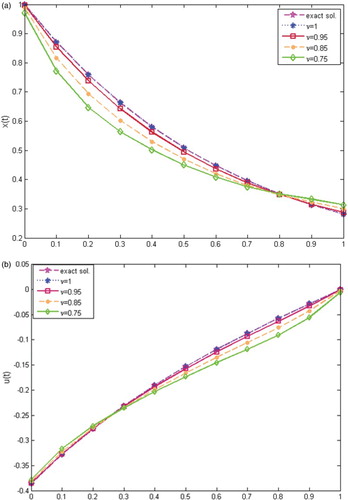
Table 1. The absolute errors of $x\left(t\right)$ for Problem 6.1 at various choices of N.

t	N=3	N=5	N=8	N=10
0	$1.25437\times {10}^{-3}$	$6.25467\times {10}^{-6}$	$6.26213\times {10}^{-10}$	$1.98861\times {10}^{-9}$
0.1	$3.30159\times {10}^{-4}$	$2.39179\times {10}^{-6}$	$1.22351\times {10}^{-10}$	$6.29444\times {10}^{-10}$
0.2	$4.86069\times {10}^{-4}$	$1.21248\times {10}^{-6}$	$3.57127\times {10}^{-11}$	$5.40695\times {10}^{-10}$
0.3	$7.78748\times {10}^{-5}$	$1.7249\times {10}^{-6}$	$1.11152\times {10}^{-10}$	$2.81709\times {10}^{-10}$
0.4	$3.34676\times {10}^{-4}$	$6.82411\times {10}^{-7}$	$1.53137\times {10}^{-10}$	$2.13957\times {10}^{-10}$
0.5	$4.57932\times {10}^{-4}$	$1.93055\times {10}^{-6}$	$6.82487\times {10}^{-12}$	$5.58041\times {10}^{-10}$
0.6	$2.30996\times {10}^{-4}$	$3.10922\times {10}^{-7}$	$1.46338\times {10}^{-10}$	$3.82721\times {10}^{-10}$
0.7	$2.02962\times {10}^{-4}$	$1.9004\times {10}^{-6}$	$1.17524\times {10}^{-10}$	$1.53133\times {10}^{-10}$
0.8	$5.2129\times {10}^{-4}$	$9.16645\times {10}^{-7}$	$2.17553\times {10}^{-11}$	$5.698\times {10}^{-10}$
0.9	$2.42861\times {10}^{-4}$	$2.49026\times {10}^{-6}$	$1.0693\times {10}^{-10}$	$7.5132\times {10}^{-10}$
1	$1.25411\times {10}^{-3}$	$6.25466\times {10}^{-6}$	$5.86238\times {10}^{-10}$	$2.68463\times {10}^{-9}$

Table 2. The absolute errors of $u\left(t\right)$ for Problem 6.1 at various choices of N.

t	N=3	N=5	N=8	N=10
0	$3.77566\times {10}^{-4}$	$1.88239\times {10}^{-6}$	$3.27507\times {10}^{-10}$	$8.1688\times {10}^{-11}$
0.1	$1.09654\times {10}^{-4}$	$7.0819\times {10}^{-7}$	$6.36999\times {10}^{-11}$	$2.70723\times {10}^{-11}$
0.2	$1.42091\times {10}^{-4}$	$3.9987\times {10}^{-7}$	$1.83641\times {10}^{-11}$	$1.54725\times {10}^{-11}$
0.3	$8.61549\times {10}^{-6}$	$4.98381\times {10}^{-7}$	$5.90761\times {10}^{-11}$	$9.72683\times {10}^{-12}$
0.4	$1.13021\times {10}^{-4}$	$2.49281\times {10}^{-7}$	$8.13922\times {10}^{-11}$	$2.06191\times {10}^{-11}$
0.5	$1.3787\times {10}^{-4}$	$5.81012\times {10}^{-7}$	$3.49132\times {10}^{-12}$	$2.08388\times {10}^{-11}$
0.6	$5.73272\times {10}^{-5}$	$4.96686\times {10}^{-8}$	$7.88284\times {10}^{-11}$	$1.56014\times {10}^{-11}$
0.7	$7.57957\times {10}^{-5}$	$5.92684\times {10}^{-7}$	$6.40287\times {10}^{-11}$	$3.26667\times {10}^{-11}$
0.8	$1.60967\times {10}^{-4}$	$2.40909\times {10}^{-7}$	$1.19774\times {10}^{-11}$	$8.78833\times {10}^{-11}$
0.9	$6.26788\times {10}^{-5}$	$7.611\times {10}^{-7}$	$5.92166\times {10}^{-11}$	$1.10133\times {10}^{-11}$
1	$3.77513\times {10}^{-4}$	$1.88239\times {10}^{-6}$	$3.25376\times {10}^{-10}$	$1.70672\times {10}^{-10}$

Problem 6.2

Consider the following FOCP [21, 32] $J=\frac{1}{2}{\int }_0^1\left(x^2\right(t)+u^2(t\left)\right)\mathrm{d}t,$ subject to $D^{\nu }x\left(t\right)=tx\left(t\right)+u\left(t\right),0\le \nu \le 1,x\left(0\right)=1.$

In Figure 2(a,b), the obtained results of the variables $x\left(t\right)$ and $u\left(t\right)$ of Problem 6.2 are plotted for different values of ν. In Table 3, comparisons of our numerical results for the minimum values of J of Problem 6.2 with different values of ν at N=8 together with the results obtained in [13] and [33] are tabulated. Obviously, our estimated results are in a good agreement with the results in [13, 33].

Figure 2. The behaviour of the approximate solutions of problem 6.2 for N=3 and $\nu =0.75,0.85,0.95,1$. (a) $x\left(t\right)$. (b) $u\left(t\right)$.

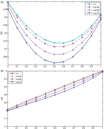
Table 3. The estimated values of J for different values of ν and N=8 for Problem 6.2.

ν	Present method	Method of [13]	Present of [33]
1	0.484268	0.48426	0.48427
0.99	0.483463	0.48346	0.48347
0.90	0.475883	0.47588	0.47605
0.80	0.466978	0.46697	0.46722

Problem 6.3

Consider the following FOCP [14] $\mathrm{Min}J={\int }_0^1(\left(x\right(t)-t^2{)}^2+(u(t)+t^4-\frac{20t^{9/10}}{9\mathrm{\Gamma }\left[\frac{9}{10}\right]}{)}^2)\mathrm{d}t,$ with the dynamic $\begin{array}{rl}{D}^{\nu }x\left(t\right)& =t^{2}x\left(t\right)+u\left(t\right),1\le \nu \le 2,\\ x\left(0\right)& =\dot{x}\left(0\right)=0.\end{array}$

Figure 3(a,b) show the approximated results of state $x\left(t\right)$ and the control $u\left(t\right)$ variables of Problem 6.3 at N=3 and $\nu =1.85,1.95$ and 2. In Table 4 comparisons of obtained results for the minimum values of J of Problem 6.3 at different choices of N together with the results obtained in [14] are tabulated. It is noted that the approximated results obtained by the suggested technique are more accurate than the results in [14].

Figure 3. The behaviour of the approximate solutions of problem 6.3 for N=3 with $\nu =1.85,1.95,2$. (a) $x\left(t\right)$. (b) $u\left(t\right)$.

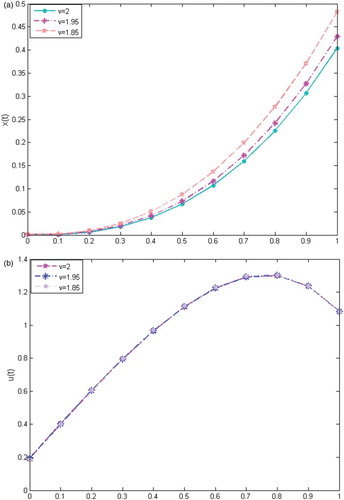
Table 4. The estimated values of J at various choices of N and $\nu =1.1$ for Problem 6.3.

N	Present method	Method of [14]
4	$2.23277\times {10}^{-6}$	$4.76932\times {10}^{-6}$
5	$8.24619\times {10}^{-7}$	$1.47243\times {10}^{-6}$
6	$3.56358\times {10}^{-7}$	$5.37825\times {10}^{-7}$
8	$9.08978\times {10}^{-8}$	$1.06099\times {10}^{-7}$
9	$5.12433\times {10}^{-8}$	$5.44304\times {10}^{-8}$

Two-Dimensional Problems

Problem 6.4

Consider the following FOCS [34] $minJ=\frac{1}{2}{\int }_0^1\left(x_1^2\right(t)+x_2^2(t)+u^2(t\left)\right)\mathrm{d}t,$ under the constraint $\begin{array}{rl}{D}^{\nu }{x}_1\left(t\right)& =-x_1\left(t\right)+x_2\left(t\right)+u\left(t\right),\\ D^{\nu }{x}_2\left(t\right)& =-2x_2\left(t\right),\\ x_1\left(0\right)& =x_2\left(0\right)=1.\end{array}$ At $\nu =1$ the exact solution is $\begin{array}{rl}{x}_1\left(t\right)& =0.018352e^{\sqrt{2}t}+2.48165e^{-\sqrt{2}t}-\frac{3e^{-2t}}{2},\\ x_2\left(t\right)& =e^{-2t},\\ u\left(t\right)& =0.044305e^{\sqrt{2}t}-1.0279322e^{-\sqrt{2}t}+\frac{e^{-2t}}{2}.\end{array}$

Figure 4(a–c) illustrate the behaviour of state variables $x_1\left(t\right),x_2\left(t\right)$ and control variable $u\left(t\right)$, respectively, for N=8 and $\nu =0.5,0.75,0.85,0.95$ and 1 with the exact solutions. Tables 5–7 display the comparison of the absolute errors by using our mechanism and the method mention in [35] of the variables $x_1\left(t\right),x_2\left(t\right)$ and $u\left(t\right)$ for Problem 6.4 at $\nu =1$ and $N=3,4,6$. These results show that the suggested method is more accurate than the results of [35]. This problem was solved in [34] by a different technique. The results shown in Figure 4(a–c) are in a good agreement with the results established in [34]. It is remarkable that we achieved satisfactory numerical results with at last 8 numbers of the SGP while in [34], number of approximations starts in 8 and increases up to 128 are used to obtain satisfactory results. So we can deduce that our numerical technique is less computational than that in [34].

Figure 4. The behaviour of the approximate solutions of problem 6.4 for N=8 and $\nu =0.65,0.75,0.85,0.95,1$, with exact solution. (a) $x1\left(t\right)$. (b) $x2\left(t\right)$. (c) $u\left(t\right)$.

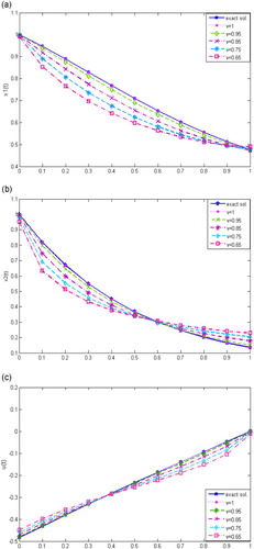
Table 5. Absolute errors of $x_1\left(t\right)$ for $\nu =1$ at various choices of N for Problem 6.4.

	Present method			Method of [35]
t	N=3	N=4	N=6	N=3	N=4	N=6
0.1	$7.4441\times {10}^{-4}$	$1.5908\times {10}^{-4}$	$7.3358\times {10}^{-7}$	$4.496\times {10}^{-4}$	$6.28\times {10}^{-5}$	$6.95\times {10}^{-6}$
0.2	$9.097\times {10}^{-4}$	$3.592\times {10}^{-5}$	$1.109\times {10}^{-6}$	$1.15\times {10}^{-3}$	$3.86\times {10}^{-4}$	$5.66\times {10}^{-6}$
0.3	$1.417\times {10}^{-5}$	$1.169\times {10}^{-4}$	$1.813\times {10}^{-7}$	$2.90\times {10}^{-3}$	$4.75\times {10}^{-4}$	$1.42\times {10}^{-6}$
0.4	$7.544\times {10}^{-4}$	$1.028\times {10}^{-4}$	$9.842\times {10}^{-7}$	$3.76\times {10}^{-3}$	$2.56\times {10}^{-4}$	$5.48\times {10}^{-7}$
0.5	$8.714\times {10}^{-4}$	$2.6567\times {10}^{-5}$	$1.395\times {10}^{-7}$	$3.34\times {10}^{-3}$	$1.14\times {10}^{-4}$	$3.54\times {10}^{-6}$
0.6	$3.19\times {10}^{-4}$	$1.2667\times {10}^{-4}$	$1.003\times {10}^{-6}$	$1.76\times {10}^{-3}$	$4.03\times {10}^{-4}$	$5.85\times {10}^{-6}$
0.7	$5.379\times {10}^{-4}$	$8.484\times {10}^{-5}$	$8.624\times {10}^{-8}$	$4.66\times {10}^{-4}$	$4.29\times {10}^{-4}$	$3.91\times {10}^{-6}$
0.8	$1.050\times {10}^{-3}$	$8.133\times {10}^{-5}$	$1.0885\times {10}^{-6}$	$2.556\times {10}^{-3}$	$1.59\times {10}^{-4}$	$1.15\times {10}^{-7}$
0.9	$3.622\times {10}^{-4}$	$1.4566\times {10}^{-4}$	$9.14\times {10}^{-7}$	$3.51\times {10}^{-3}$	$2.14\times {10}^{-4}$	$1.84\times {10}^{-6}$

Table 6. Absolute errors of $x_2\left(t\right)$ for $\nu =1$ at different choices of N for Problem 6.4.

	Present method			Method of [35]
t	N=3	N=4	N=6	N=3	N=4	N=6
0.1	$1.044\times {10}^{-3}$	$1.68\times {10}^{-4}$	$6.053\times {10}^{-7}$	$7.18\times {10}^{-4}$	$5.97\times {10}^{-5}$	$1.80\times {10}^{-6}$
0.2	$1.41\times {10}^{-3}$	$4.112\times {10}^{-5}$	$9.0967\times {10}^{-7}$	$1.6\times {10}^{-3}$	$4.06\times {10}^{-4}$	$1.28\times {10}^{-6}$
0.3	$1.357\times {10}^{-4}$	$1.226\times {10}^{-4}$	$1.430\times {10}^{-7}$	$4.40\times {10}^{-3}$	$5.105\times {10}^{-4}$	$1.75\times {10}^{-6}$
0.4	$1.059\times {10}^{-3}$	$1.114\times {10}^{-4}$	$8.085\times {10}^{-7}$	$6.02\times {10}^{-3}$	$2.878\times {10}^{-4}$	$2.109\times {10}^{-6}$
0.5	$1.338\times {10}^{-3}$	$2.47\times {10}^{-5}$	$1.08\times {10}^{-7}$	$5.81\times {10}^{-3}$	$1.04\times {10}^{-4}$	$6.6\times {10}^{-7}$
0.6	$5.927\times {10}^{-4}$	$1.336\times {10}^{-4}$	$8.232\times {10}^{-7}$	$3.81\times {10}^{-3}$	$4.21\times {10}^{-4}$	$2.87\times {10}^{-6}$
0.7	$6.9627\times {10}^{-4}$	$9.2876\times {10}^{-5}$	$6.467\times {10}^{-8}$	$6.66\times {10}^{-4}$	$4.649\times {10}^{-4}$	$1.555\times {10}^{-6}$
0.8	$1.562\times {10}^{-3}$	$8.327\times {10}^{-5}$	$8.9367\times {10}^{-7}$	$2.52\times {10}^{-3}$	$1.924\times {10}^{-4}$	$1.528\times {10}^{-6}$
0.9	$6.41\times {10}^{-4}$	$1.557\times {10}^{-4}$	$7.455\times {10}^{-7}$	$4.22\times {10}^{-3}$	$1.99\times {10}^{-4}$	$1.29\times {10}^{-6}$

Table 7. Absolute error of $u\left(t\right)$ for $\nu =1$ at different values of N for Problem 6.4.

	Present method			Method of [35]
t	N=3	N=4	N=6	N=3	N=4	N=6
0.1	$2.308\times {10}^{-4}$	$3.77\times {10}^{-5}$	$2.124\times {10}^{-7}$	$1.88\times {10}^{-4}$	$1.05\times {10}^{-5}$	$2.6\times {10}^{-6}$
0.2	$3.136\times {10}^{-4}$	$6.07\times {10}^{-6}$	$3.267\times {10}^{-7}$	$3.5\times {10}^{-4}$	$8.06\times {10}^{-5}$	$2.12\times {10}^{-6}$
0.3	$3.199\times {10}^{-5}$	$2.869\times {10}^{-5}$	$5.86\times {10}^{-8}$	$9.96\times {10}^{-4}$	$8.94\times {10}^{-5}$	$8.6\times {10}^{-7}$
0.4	$2.316\times {10}^{-4}$	$2.253\times {10}^{-5}$	$2.890\times {10}^{-7}$	$1.4\times {10}^{-4}$	$2.6\times {10}^{-5}$	$5.09\times {10}^{-7}$
0.5	$2.942\times {10}^{-4}$	$8.891\times {10}^{-6}$	$4.657\times {10}^{-8}$	$1.4\times {10}^{-3}$	$6.7\times {10}^{-5}$	$1.35\times {10}^{-6}$
0.6	$1.313\times {10}^{-4}$	$3.054\times {10}^{-5}$	$2.95\times {10}^{-7}$	$1.1\times {10}^{-3}$	$1.34\times {10}^{-5}$	$1.96\times {10}^{-6}$
0.7	$1.53\times {10}^{-4}$	$1.797\times {10}^{-5}$	$3.07\times {10}^{-8}$	$4.22\times {10}^{-4}$	$1.35\times {10}^{-4}$	$1.32\times {10}^{-6}$
0.8	$3.446\times {10}^{-4}$	$2.124\times {10}^{-5}$	$3.198\times {10}^{-7}$	$1.97\times {10}^{-4}$	$6.88\times {10}^{-5}$	$9.16\times {10}^{-6}$
0.9	$1.401\times {10}^{-4}$	$3.32\times {10}^{-5}$	$2.727\times {10}^{-7}$	$4.78\times {10}^{-4}$	$1.38\times {10}^{-5}$	$1.0\times {10}^{-7}$

Three-Dimensional Problem

Problem 6.5

Consider the following FOCS ([36]) $minJ=\frac{1}{2}{\int }_0^1\left(x_1^2\right(t)+x_2^2(t)-x_3^2(t)+u^2(t\left)\right)\mathrm{d}t$ with the dynamic constraints $\begin{array}{rl}{D}^{\nu }{x}_1\left(t\right)& =-2x_1\left(t\right)-t{x}_2\left(t\right)+u\left(t\right),\\ D^{\nu }{x}_2\left(t\right)& =3x_1\left(t\right)+x_3\left(t\right)-u\left(t\right),\\ D^{\nu }{x}_3\left(t\right)& =t{x}_1\left(t\right)+x_2\left(t\right),\\ x_1\left(0\right)& =x_2\left(0\right)=x_3\left(0\right)=1.\end{array}$

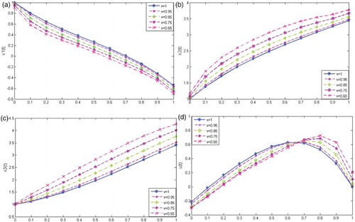
Figure 5(a–d) illustrate the behaviour of approximate solution of the variables $x_1\left(t\right),x_2\left(t\right),x_3\left(t\right)$ and $u\left(t\right)$, respectively, for N=5 at various choices of ν ($\nu =0.65,0.75,0.85,0.95$ and 1).

Figure 5. The behaviour of the approximate solutions of problem 6.5 for N=5 and $\nu =0.65,0.75,0.85,0.95,1$. (a) $x1\left(t\right)$. (b) $x2\left(t\right)$. (c) $x3\left(t\right)$. (d) $u\left(t\right)$.

7. Conclusions

In this paper, a new numerical mechanism has been derived to find the approximate solutions of the multi-dimensional FOCPs, this numerical mechanism depends on the SGOM of RLFI. The SGOM of fractional integration reduced the FOCP into an equivalent integral problem. The properties of the SGPs together with the LMM are used to transform the equivalent functional integral equation problem into an algebraic system of equations, which is easily to solve. The applicability, accuracy and rapidity by using few terms of the SGPs of the proposed mechanism are illustrated by numerical applications and the numerical comparisons with some existing methods in the literatures.

Disclosure statement

No potential conflict of interest was reported by the author.

ORCID

Hoda F. Ahmed  http://orcid.org/0000-0001-8930-1296

References

- Bohannan GW. Analog fractional order controller in temperature and motor control applications. J Vib Control. 2008;14(9–10):1487–1498.
- Suarez JI, Vinagre BM, Chen Y. A fractional adaptation scheme for lateral control of an AGV. J Vib Control. 2008;14(9–10):1499–1511.
- Atanackovic TM, Pilipovic S, Stankovic B, et al. Fractional calculus with applications in mechanics: wave propagation, impact and variational principles. New York (NY): Wiley; 2014.
- Machado JAT, Silva MF, Barbosa RS, et al. Some applications of fractional calculus in engineering. Math Prob Eng. 2010;2010:1–34.
- Kilbas AA, Srivastava HM, Trujillo JJ. Theory and applications of fractional differential equations. San Diego (CA): Elsevier; 2006.
- Jesus IS, Machado JT. Fractional control of heat diffusion systems. Nonlinear Dyn. 2008;54:263–282.
- Agrawal OP. Fractional optimal control of a distributed system using eigenfunctions. J Comput Nonlinear Dyn. 2008;3(2):021204.
- Tricaud C, Chen Y. An approximate method for numerically solving fractional order optimal control problems of general form. Comput Math Appl. 2010;59(5):1644–1655.
- Debbouche A, Nieto JJ, Torres DF. Optimal solutions to relaxation in multiple control problems of Sobolev type with nonlocal nonlinear fractional differential equations. J Optim Theory Appl. 2017;174(1):7–31.
- Bhrawy AH, Doha EH, Baleanu D, et al. A spectral tau algorithm based on Jacobi operational matrix for numerical solution of time fractional diffusion-wave equations. J Comput Phys. 2015;293:142–156.
- Erjaee GH, Akrami MH, Atabakzadeh MH. The operational matrix of fractional integration for shifted Legendre polynomials. Iranian J Sci Technol (Sciences). 2013;37(4):439–444.
- Nemati A, Yousefi S, Soltanian F, et al. An efficient numerical solution of fractional optimal control problems by using the Ritz method and Bernstein operational matrix. Asian J Control. 2016;18(6):2272–2282.
- Doha EH, Bhrawy AH, Ezz-Eldien SS. A Chebyshev spectral method based on operational matrix for initial and boundary value problems of fractional order. Comput Math Appl. 2011;62(5):2364–2373.
- Bhrawy AH, Alofi AS. The operational matrix of fractional integration for shifted Chebyshev polynomials. Appl Math Lett. 2013;26(1):25–31.
- Saadatmandi A, Dehghan M. A new operational matrix for solving fractional-order differential equations. Comput Math Appl. 2010;59(3):1326–1336.
- Doha EH, Bhrawy AH, Ezz-Eldien SS. A new Jacobi operational matrix: an application for solving fractional differential equations. Appl Math Model. 2012;36(10):4931–4943.
- Bhrawy AH, Tharwat MM, Alghamdi MA. A new operational matrix of fractional integration for shifted Jacobi polynomials. Bull Malays Math Sci Soc. 2014;37(4):983–995.
- Saadatmandi A. Bernstein operational matrix of fractional derivatives and its applications. Appl Math Model. 2014;38(4):1365–1372.
- Bhrawy AH, Baleanu D, Assas LM. Efficient generalized Laguerre-spectral methods for solving multi-term fractional differential equations on the half line. J Vib Control. 2014;20(7):973–985.
- Kucuk I, Sadek I. An efficient computational method for the optimal control problem for the Burgers equation. Math Comput Model. 2006;44(11):973–982.
- Lotfi A, Dehghan M, Yousefi SA. A numerical technique for solving fractional optimal control problems. Comput Math Appl. 2011;62(3):1055–1067.
- Maleknejad K, Almasieh H. Optimal control of Volterra integral equations via triangular functions. Math Comput Model. 2011;53(9):1902–1909.
- Maleknejad K, Hashemizadeh E, Basirat B. Computational method based on Bernstein operational matrices for nonlinear Volterra–Fredholm–Hammerstein integral equations. Commun Nonlinear Sci Numer Simul. 2012;17(1):52–61.
- El-Hawary HM, Salim MS, Hussien HS. An optimal ultraspherical approximation of integrals. Int J Comp Math. 2000;76(2):219–237.
- El-Kady MM, Hussien HS, Ibrahim MA. Ultraspherical spectral integration method for solving linear integro-differential equations. Int J Appl Math Comput Sci. 2009;5:1.
- Elgindy KT. High order numerical solution of second order one dimensional hyperbolic telegraph equation using a shifted Gegenbauer pseudospectral method. Numer Methods Partial Differ Equ. 2016;32(1):307–349.
- Elgindy KT, Smith-Miles KA. Optimal Gegenbauer quadrature over arbitrary integration nodes. J Comput Appl Math. 2013;242:82–106.
- Miller KS, Ross B. An introduction to the fractional calculus and fractional differential equations. Wiley-Interscience; 1993.
- Kreyszig E. Introductory functional analysis with applications. New York (NY): Wiley; 1989.
- Rivlin TJ. An introduction to the approximation of functions. New York: Dover-Publications-Inc; 2003.
- Phang C, Ismail NF, Isah A, et al. A new efficient numerical scheme for solving fractional optimal control problems via a Genocchi operational matrix of integration. J Vib Control. 2017. https://doi.org/10.1177/1077546317698909
- Agrawal OP. A general formulation and solution scheme for fractional optimal control problems. Nonlinear Dyn. 2004;38(1–4):323–337.
- Akbarian T, Keyanpour M. A new approach to the numerical solution of fractional order optimal control problems. Appl Appl Math. 2013;8:523–534.
- Defterli O. A numerical scheme for two-dimensional optimal control problems with memory effect. Comput Math Appl. 2010;59(5):1630–1636.
- Yousefi SA, Lotfi A, Dehghan M. The use of a Legendre multiwavelet collocation method for solving the fractional optimal control problems. J Vib Control. 2011;17(13):2059–2065.
- Bhrawy AH, Doha EH, Tenreiro Machado JA, et al. An efficient numerical scheme for solving multi-dimensional fractional optimal control problems with a quadratic performance index. Asian J Control. 2015;17(6):2389–2402.