Boundary controllability of impulsive integrodifferential evolution systems with time-varying delays

ABSTRACT

In this paper, authors studied the boundary controllability results for neutral impulsive integrodifferential evolution systems with time-varying delays in Banach spaces. The sufficient conditions of the boundary controllability are proved under the evolution operator. The results are obtained by using the semigroup theory and the Schaefer fixed point theorems.

Keywords:

• Boundary controllability
• impulsive integrodifferential system
• evolution operator
• time-varying delay
• semigroup theory
• fixed point theorem

2010 AMS Subject Classification::

• 93B05
• 47D06
• 47H10
• 35R12

1. Introduction

The theory of differential equations in abstract spaces is a fascinating field with important applications to a number of areas of analysis and other branches of mathematics. Depending on the nature of the problems, these equations may take various forms such as ordinary differential equations. Using the method of semigroups, various solutions of nonlinear and semilinear evolution equations have been discussed by Pazy [1]. Delay differential equations are similar to ordinary differential equation, but their evolution involves past values of the state variable. Time delay is inherently the character of most dynamical systems to some extent. Time delays are frequently encountered in various engineering systems such as aircraft, long transmission lines in pneumatic models and chemical or process control systems. These delays may be the source of instability and lead to serious deterioration in the performance of closed-loop systems. The problem of controllability of nonlinear systems and integrodifferential systems including delay systems has been studied by many researchers [2–4] and the theory of neutral differential equations has been studied by the authors Radhakrishnan and Balachandran [5].

The concept of control can be described as the process of influencing the behaviour of a dynamical system so as to achieve a desired goal. Roughly speaking, controllability generally means that it is possible to steer a dynamical system from an arbitrary initial state to an arbitrary final state using the set of admissible controls. The complexity of modern systems, inaccuracies in output measurements and uncertainties about the system dynamics often make this problem extremely hard to solve. Controllability of linear and nonlinear systems represented by ordinary differential equations in finite-dimensional spaces has been extensively investigated. Since there are many examples where time delay and spatial diffusion enter the control systems, several authors have extended the concept of controllability to infinite-dimensional systems in Banach spaces [6].

The fast scientific development in the foundations and micro-world of biology has led to a reconsideration of nature and some characteristics of life. In fact, scientists agree that its continuous nature in enriched by discretely arising discontinuities and the latter ones are also called jumps or impulses. The dynamics of many evolving processes are subject to abrupt changes, such as shocks, harvesting and natural disasters. These phenomena involve short-term perturbations from continuous and smooth dynamics, whose duration is negligible in comparison with the duration of an entire evolution. For more details on this theory and on its applications, we refer to the monographs of Lakshmikantham et al. [7], and Samoilenko and Perestyuk [8] for the case of ordinary impulsive systems and [9] for partial differential equations with impulsive systems. Similarly in [10], the authors discussed the abstract neutral differential equation with time-varying delay by using the Schaefer fixed point theorem.

The study on the distributed control systems in which the control is exercised through the boundary as distinct from systems controlled in the interior has emerged as one of the most important fields of modern research. Many partial integrodifferential equations with boundary control occur frequently in various physical applications like evolution of population, modelling of thermoelastic plates and damped wave equations. These types of physical models can be reformulated mathematically into an abstract smooth function. Several authors [11,12] have developed many abstract settings to describe the boundary control systems in which the control must be taken in sufficiently smooth functions for the existence of regular solutions to state space system. A semigroup approach to boundary input problems for linear differential equations was developed by Fattorini [13] and Washburn [14]. In [15] Barbu discussed a class of boundary-distributed linear control systems in Banach Spaces. The problem of boundary controllability of integrodifferential systems and delay integrodifferential systems in Banach spaces has been investigated by Balachandran and Anandhi [16,17].

The purpose of this paper is to establish the set sufficient conditions for the boundary controllability of neutral impulsive integrodifferential evolution systems with time-varying delays by using the semigroup theory and fixed point theorem.

2. Preliminaries

Let $\mathbb{X}$ and $\mathbb{Y}$ be a pair of real Banach spaces with the norms $\parallel \cdot {\parallel }_{\mathbb{X}}$ and $\parallel \cdot {\parallel }_{\mathbb{Y}}$, respectively. Let α be linear, closed and densely defined operator with $D\left(\alpha \right)\subseteq \mathbb{X}$ and $R\left(\alpha \right)\subseteq \mathbb{X}$ and let θ be a linear operator with $\mathcal{D}\left(\theta \right)\subseteq \mathbb{X}$ and $\mathcal{R}\left(\theta \right)\subseteq \mathbb{E},$ a Banach space.

Throughout this paper, $(\mathbb{X},\parallel \cdot \parallel )$ is a Banach space, $\left\{A\right(t):t\in \mathbb{R}\}$ is a family of closed linear operators defined on a common domain $\mathcal{D}$ which is dense in $\mathbb{X}$ and we assume that the linear non-autonomous system (1) $\begin{array}{rl}{x}^{\mathrm{\prime }}\left(t\right)& =A\left(t\right)x\left(t\right),s\le t\le b,\\ x\left(s\right)& =w\in \mathbb{X}\end{array}$(1) has associated evolution family of operators $\left\{U\right(t,s):0\le s\le t\le b\}$. In the next definition, $\mathcal{L}\left(\mathbb{X}\right)$ is a space of bounded linear operator from $\mathbb{X}$ into $\mathbb{X}$ endowed with the uniform convergence topology.

Definition 2.1

[1] A family of operators $\left\{U\right(t,s):0\le s\le t\le b\}\subset \mathcal{L}\left(\mathbb{X}\right)$ is called a evolution family of bounded linear operators for (1(1) $\begin{array}{rl}{x}^{\mathrm{\prime }}\left(t\right)& =A\left(t\right)x\left(t\right),s\le t\le b,\\ x\left(s\right)& =w\in \mathbb{X}\end{array}$(1) ) if the following properties hold:

1. $\parallel U(t,s)\parallel \le \exp ({\displaystyle {\int }_s^t\parallel A\left(\tau \right)\parallel \mathrm{d}\tau ).}$

2. $U(t,s)U(s,\tau )=U(t,\tau )$ and $U(t,t)x=x$, for every $s\le \tau \le t$ and all $x\in \mathbb{X}$.

3. For each $x\in \mathbb{X},$ the function for $(t,s)\to U(t,s)x$ is continuous and $U(t,s)\in \mathcal{L}\left(\mathbb{X}\right),$ for every $t\ge s.$

4. For $0\le s\le t\le b,$ the function $t\to U(t,s),$ for $(s,t]\in \mathcal{L}\left(\mathbb{X}\right),$ is differentiable with ${\displaystyle \mathrm{\partial }/\mathrm{\partial }tU(t,s)=A\left(t\right)U(t,s).}$

5. ${\displaystyle \mathrm{\partial }/\mathrm{\partial }sU(t,s)=-U(t,s)A\left(s\right),}$ for $0\le s\le t\le b.$

To accommodate the impulsive condition in the system, it is convenient to introduce some additional concepts and notations.

Let $J_0=[0,t_1],J_i=(t_i,t_{i+1}],i=1,2,\dots ,m$ and define the following spaces:Let $\mathcal{P}\mathcal{C}\left(\right[0,b],\mathbb{X})$= $\{x:x$ is a function from $[0,b]$ into $\mathbb{X}$ such that $x\left(t\right)$ is continuous at $t\ne t_i$ and left continuous at $t=t_i$ and the right limit $x\left(t_i^{+}\right)$ exists, for $i=1,2\dots m\}$. Similarly as in [18], we see that $\mathcal{P}\mathcal{C}\left(\right[0,b],\mathbb{X})$ is a Banach space with the norm $\parallel x{\parallel }_{\mathcal{P}\mathcal{C}}=\underset{t\in [0,b]}{sup}\parallel x\left(t\right)\parallel .$

To prove the boundary controllability results we need the following hypotheses:

1. $\mathcal{D}\left(\alpha \right)\subset \mathcal{D}\left(\theta \right)$ and the restriction of θ to $\mathcal{D}\left(\alpha \right)$ is continuous relative to graph norm of $\mathcal{D}\left(\alpha \right)$.

2. $A\left(t\right)$ generates a family of evolution operators $U(t,s),$ when $t>s>0,$ of $C_0$ semigroup on $\mathbb{X}$ and there exists a constant M>0 such that $\parallel U(t,s)\parallel \le M\text{for}0\le s\le t\le b.$

3. There exists a linear continuous operator $B:\mathbb{Y}\to \mathbb{X}$ such that $\alpha B\in \mathcal{L}(\mathbb{Y},\mathbb{X})$, $\theta \left(Bu\right)=B_{1}u$, for all $u\in \mathbb{Y}.$ Also $Bu\left(t\right)$ is continuously differentiable and $\parallel Bu\parallel \le C\parallel B_{1}u\parallel ,$ for all $u\in \mathbb{Y}$, where C is a constant.

4. For all $t\in (0,b]$ and $u\in \mathbb{Y},$ $U(t,s)Bu\in \mathcal{D}\left(A\right).$ Moreover, there exists a positive function $\nu \in {\mathcal{L}}^1(0,b)$ such that $\parallel A\left(s\right)U(t,s)B\parallel \in \nu \left(t\right)$, a.e. for $t\in (0,b)$ and choose a constant P>0 such that ${\int }_0^b\nu \left(t\right)\mathrm{d}t\le P.$

5. $h:J\times \mathbb{X}\times \mathbb{X}\to \mathbb{X}$ is continuously differentiable and $U(t,s)h(s,x,y)\in \mathcal{D}\left(A\right),$ and for each $s\in [0,t),$ the function $A\left(s\right)U(t,s)h(s,x(s),x(\cdot \left)\right)$ is integrable.

Consider the first-order boundary control neutral impulsive integrodifferential evolution system of the form (2) $\begin{array}{rl}& \frac{\mathrm{d}}{\mathrm{d}t}\left[x\right(t)+h(t,x\left(t\right),x\left({\sigma }_1\right(t\left)\right)]\\ & =\alpha \left(t\right)x\left(t\right)+f(t,x(t),x({\sigma }_2\left(t\right)\left)\right)\\ & +{\int }_0^{t}g(t,s,x({\sigma }_3\left(s\right)\left)\right)\mathrm{d}s,t\ne t_i,t\in J=[0,b],\\ & x\left(0\right)=x_0,\\ & \theta x\left(t\right)=B_{1}u\left(t\right),t\in J=[0,b],\\ & \mathrm{\Delta }x{|}_{t=t_i}=I_i\left(x\right(t_i^{-}\left)\right),i=1,2,\dots m,\end{array}$(2) where the state variable $x(\cdot )$ takes values in the Banach space $\mathbb{X}$ with norm $\parallel \cdot \parallel$ and the control function $u(\cdot )$ is given in ${\mathbb{L}}^2(J,\mathbb{Y})$, a Banach space of admissible control functions $B_1:\mathbb{Y}\to \mathbb{X}$ is a linear continuous operator and the nonlinear operators and $J=[0,b],\mathrm{\Delta }=\left\{\right(t,s):0\le s\le t\le b\}$. Here $A\left(t\right)$ closed operators on $\mathbb{X}$ with dense domain $\mathcal{D}\left(A\right(t\left)\right)$ which is independent of $t;h:J\times \mathbb{X}\times \mathbb{X}\to \mathbb{X},$ $f:J\times \mathbb{X}\times \mathbb{X}\to \mathbb{X},g:\mathrm{\Delta }\times \mathbb{X}\to \mathbb{X},I_i:\mathbb{X}\to \mathbb{X}.$ The delays ${\sigma }_1,{\sigma }_2,{\sigma }_3$ are given appropriate functions; $x\left(t_i^{+}\right)$ and $x\left(t_i^{-}\right)$ represent the right and left limits of $x\left(t\right)$ at $t=t_i$ for $0=t_0<t_1\cdots <t_i<t_{i+1}=b.$

Let $x\left(t\right)$ be the solution of (2(2) $\begin{array}{rl}& \frac{\mathrm{d}}{\mathrm{d}t}\left[x\right(t)+h(t,x\left(t\right),x\left({\sigma }_1\right(t\left)\right)]\\ & =\alpha \left(t\right)x\left(t\right)+f(t,x(t),x({\sigma }_2\left(t\right)\left)\right)\\ & +{\int }_0^{t}g(t,s,x({\sigma }_3\left(s\right)\left)\right)\mathrm{d}s,t\ne t_i,t\in J=[0,b],\\ & x\left(0\right)=x_0,\\ & \theta x\left(t\right)=B_{1}u\left(t\right),t\in J=[0,b],\\ & \mathrm{\Delta }x{|}_{t=t_i}=I_i\left(x\right(t_i^{-}\left)\right),i=1,2,\dots m,\end{array}$(2) ). Then, we can define a function $z\left(t\right)=x\left(t\right)-Bu\left(t\right)$ and, from our assumption, we see that $z\left(t\right)\in \mathcal{D}\left(A\right)$. Hence, (2(2) $\begin{array}{rl}& \frac{\mathrm{d}}{\mathrm{d}t}\left[x\right(t)+h(t,x\left(t\right),x\left({\sigma }_1\right(t\left)\right)]\\ & =\alpha \left(t\right)x\left(t\right)+f(t,x(t),x({\sigma }_2\left(t\right)\left)\right)\\ & +{\int }_0^{t}g(t,s,x({\sigma }_3\left(s\right)\left)\right)\mathrm{d}s,t\ne t_i,t\in J=[0,b],\\ & x\left(0\right)=x_0,\\ & \theta x\left(t\right)=B_{1}u\left(t\right),t\in J=[0,b],\\ & \mathrm{\Delta }x{|}_{t=t_i}=I_i\left(x\right(t_i^{-}\left)\right),i=1,2,\dots m,\end{array}$(2) ) can be written in terms of A and B as $\begin{array}{rl}& \frac{\mathrm{d}}{\mathrm{d}t}\left[x\right(t)+h(t,x\left(t\right),x\left({\sigma }_1\right(t\left)\right)\left)\right]\\ & =A\left(t\right)z\left(t\right)+\alpha \left(t\right)Bu\left(t\right)+f(t,x(t),x({\sigma }_2\left(t\right)\left)\right)\\ & +{\int }_0^{t}g(t,s,x({\sigma }_3\left(t\right)\left)\right)\mathrm{d}s,\\ & t\ne t_i,t\in J=[0,b],\\ x\left(t\right)& =z\left(t\right)+Bu\left(t\right),\\ x\left(0\right)& =x_0,\\ \mathrm{\Delta }x{|}_{t=t_i}& =I_i\left(x\right(t_i^{-}\left)\right),i=1,2,\dots m.\end{array}$ If u is a continuously differentiable on $[0,b],$ then z can be defined as a mild solution to the Cauchy problem $\begin{array}{rl}\dot{z}\left(t\right)& =A\left(t\right)z\left(t\right)+\alpha \left(t\right)Bu\left(t\right)-\frac{\mathrm{d}}{\mathrm{d}t}\left[h\right(t,x\left(t\right),x\left({\sigma }_1\right(t\left)\right)]\\ & +f(t,x(t),x({\sigma }_2\left(t\right)\left)\right)\\ & +{\int }_0^{t}g(t,s,x({\sigma }_3\left(t\right)\left)\right)\mathrm{d}s-B{u}^{\mathrm{\prime }}\left(t\right),\\ z\left(0\right)& =x_0-Bu\left(0\right),\\ \mathrm{\Delta }x{|}_{t=t_i}& =I_i\left(x\right(t_i^{-}\left)\right),i=1,2,\dots m,\end{array}$ and the solution of (2(2) $\begin{array}{rl}& \frac{\mathrm{d}}{\mathrm{d}t}\left[x\right(t)+h(t,x\left(t\right),x\left({\sigma }_1\right(t\left)\right)]\\ & =\alpha \left(t\right)x\left(t\right)+f(t,x(t),x({\sigma }_2\left(t\right)\left)\right)\\ & +{\int }_0^{t}g(t,s,x({\sigma }_3\left(s\right)\left)\right)\mathrm{d}s,t\ne t_i,t\in J=[0,b],\\ & x\left(0\right)=x_0,\\ & \theta x\left(t\right)=B_{1}u\left(t\right),t\in J=[0,b],\\ & \mathrm{\Delta }x{|}_{t=t_i}=I_i\left(x\right(t_i^{-}\left)\right),i=1,2,\dots m,\end{array}$(2) ) is given by (3) $\begin{array}{rl}x\left(t\right)& =U(t,0)[x_0-Bu(0\left)\right]\\ & +{\int }_0^{t}U(t,s)\left[\alpha \right(s\left)Bu\right(s)-B{u}^{\mathrm{\prime }}(s\left)\right]\mathrm{d}s+Bu\left(t\right)\\ & -{\int }_0^{t}U(t,s)\frac{\mathrm{d}}{\mathrm{d}s}h(s,x(s),x({\sigma }_1\left(s\right)\left)\right)\mathrm{d}s\\ & +{\int }_0^{t}U(t,s)f(s,x(s),x({\sigma }_2\left(s\right)\left)\right)\mathrm{d}s\\ & +{\int }_0^{t}U(t,s)\left[{\int }_0^{s}g(s,\tau ,x({\sigma }_3\left(\tau \right)\left)\right)\mathrm{d}\tau \right]\mathrm{d}s\\ & +\sum _{0<t_i<t}U(t,t_i)I_i\left(x\right(t_i^{-}\left)\right).\end{array}$(3)

Definition 2.2

A solution $x(\cdot )\in \mathcal{P}\mathcal{C}\left(\right[0,b],\mathbb{X})$ is said to be a mild solution of (2(2) $\begin{array}{rl}& \frac{\mathrm{d}}{\mathrm{d}t}\left[x\right(t)+h(t,x\left(t\right),x\left({\sigma }_1\right(t\left)\right)]\\ & =\alpha \left(t\right)x\left(t\right)+f(t,x(t),x({\sigma }_2\left(t\right)\left)\right)\\ & +{\int }_0^{t}g(t,s,x({\sigma }_3\left(s\right)\left)\right)\mathrm{d}s,t\ne t_i,t\in J=[0,b],\\ & x\left(0\right)=x_0,\\ & \theta x\left(t\right)=B_{1}u\left(t\right),t\in J=[0,b],\\ & \mathrm{\Delta }x{|}_{t=t_i}=I_i\left(x\right(t_i^{-}\left)\right),i=1,2,\dots m,\end{array}$(2) ) if $x\left(0\right)=x_0,t\in [0,b],\mathrm{\Delta }x{|}_{t=t_i}=I_i\left(x\right(t_i^{-}\left)\right),i=1,2,\dots ,m$; the restriction of $x(\cdot )$ to the interval $J_i(i=0,1,\dots ,m)$ is continuous and, for each $0\le t\le b,$ the function $U(t,s)A\left(s\right)h(s,x(s),x({\sigma }_1\left(s\right)\left)\right),s\in [0,t),$ is integrable and the following integral equation: (4) $\begin{array}{rl}x\left(t\right)& =U(t,0)[x_0+h(0,x\left(0\right),x\left({\sigma }_1\right(0\left)\right)\left)\right]\\ & -h(t,x(t),x({\sigma }_1\left(t\right)\left)\right)\\ & -{\int }_0^{t}U(t,s)A\left(s\right)h(s,x(s),x({\sigma }_1\left(s\right)\left)\right)\mathrm{d}s\\ & +{\int }_0^t\left[U\right(t,s\left)\alpha \right(s)-U(t,s\left)A\right(s\left)\right]Bu\left(s\right)\mathrm{d}s\\ & +{\int }_0^{t}U(t,s)f(s,x(s),x({\sigma }_2\left(s\right)\left)\right)\mathrm{d}s\\ & +{\int }_0^{t}U(t,s)\left[{\int }_0^{s}g(s,\tau ,x({\sigma }_3\left(\tau \right)\left)\right)\mathrm{d}\tau \right]\mathrm{d}s\\ & +\sum _{0<t_i<t}U(t,t_i)I_i\left(x\right(t_i^{-}\left)\right).\end{array}$(4) Thus, (4(4) $\begin{array}{rl}x\left(t\right)& =U(t,0)[x_0+h(0,x\left(0\right),x\left({\sigma }_1\right(0\left)\right)\left)\right]\\ & -h(t,x(t),x({\sigma }_1\left(t\right)\left)\right)\\ & -{\int }_0^{t}U(t,s)A\left(s\right)h(s,x(s),x({\sigma }_1\left(s\right)\left)\right)\mathrm{d}s\\ & +{\int }_0^t\left[U\right(t,s\left)\alpha \right(s)-U(t,s\left)A\right(s\left)\right]Bu\left(s\right)\mathrm{d}s\\ & +{\int }_0^{t}U(t,s)f(s,x(s),x({\sigma }_2\left(s\right)\left)\right)\mathrm{d}s\\ & +{\int }_0^{t}U(t,s)\left[{\int }_0^{s}g(s,\tau ,x({\sigma }_3\left(\tau \right)\left)\right)\mathrm{d}\tau \right]\mathrm{d}s\\ & +\sum _{0<t_i<t}U(t,t_i)I_i\left(x\right(t_i^{-}\left)\right).\end{array}$(4) ) is well defined and it is called mild of solution of the system (2(2) $\begin{array}{rl}& \frac{\mathrm{d}}{\mathrm{d}t}\left[x\right(t)+h(t,x\left(t\right),x\left({\sigma }_1\right(t\left)\right)]\\ & =\alpha \left(t\right)x\left(t\right)+f(t,x(t),x({\sigma }_2\left(t\right)\left)\right)\\ & +{\int }_0^{t}g(t,s,x({\sigma }_3\left(s\right)\left)\right)\mathrm{d}s,t\ne t_i,t\in J=[0,b],\\ & x\left(0\right)=x_0,\\ & \theta x\left(t\right)=B_{1}u\left(t\right),t\in J=[0,b],\\ & \mathrm{\Delta }x{|}_{t=t_i}=I_i\left(x\right(t_i^{-}\left)\right),i=1,2,\dots m,\end{array}$(2) ).

Definition 2.3

The system (2(2) $\begin{array}{rl}& \frac{\mathrm{d}}{\mathrm{d}t}\left[x\right(t)+h(t,x\left(t\right),x\left({\sigma }_1\right(t\left)\right)]\\ & =\alpha \left(t\right)x\left(t\right)+f(t,x(t),x({\sigma }_2\left(t\right)\left)\right)\\ & +{\int }_0^{t}g(t,s,x({\sigma }_3\left(s\right)\left)\right)\mathrm{d}s,t\ne t_i,t\in J=[0,b],\\ & x\left(0\right)=x_0,\\ & \theta x\left(t\right)=B_{1}u\left(t\right),t\in J=[0,b],\\ & \mathrm{\Delta }x{|}_{t=t_i}=I_i\left(x\right(t_i^{-}\left)\right),i=1,2,\dots m,\end{array}$(2) ) is said to be controllable on the interval J if for every $x_0,x_b\in \mathbb{X},$ there exists a control $u\in {\mathcal{L}}^2(J,\mathbb{Y})$ such that the solution $x(\cdot )$ of (2(2) $\begin{array}{rl}& \frac{\mathrm{d}}{\mathrm{d}t}\left[x\right(t)+h(t,x\left(t\right),x\left({\sigma }_1\right(t\left)\right)]\\ & =\alpha \left(t\right)x\left(t\right)+f(t,x(t),x({\sigma }_2\left(t\right)\left)\right)\\ & +{\int }_0^{t}g(t,s,x({\sigma }_3\left(s\right)\left)\right)\mathrm{d}s,t\ne t_i,t\in J=[0,b],\\ & x\left(0\right)=x_0,\\ & \theta x\left(t\right)=B_{1}u\left(t\right),t\in J=[0,b],\\ & \mathrm{\Delta }x{|}_{t=t_i}=I_i\left(x\right(t_i^{-}\left)\right),i=1,2,\dots m,\end{array}$(2) ) satisfies $x\left(0\right)=x_0$ and $x\left(b\right)=x_b.$

Theorem 2.4

For arbitrary $x\left(t\right)\in \mathbb{X},$ define the control (5) $\begin{array}{rl}u\left(t\right)& ={\mathbb{W}}^{-1}\left[x_b-U(b,0)[x_0+h(0,x\left(0\right),x\left({\sigma }_1\right(0\left)\right)\left)\right]\phantom{\sum _{0<t_i<t}U(b,t_i)I_i\left(x\right(t_i^{-}\left)\right)}\right.\\ & +h(b,x(b),x({\sigma }_1\left(b\right)\left)\right)\\ & +{\int }_0^{b}U(b,\eta )A\left(\eta \right)h(\eta ,x(\eta ),x({\sigma }_1\left(\eta \right)\left)\right)\mathrm{d}\eta \\ & -{\int }_0^{b}U(b,\eta )f(\eta ,x(\eta ),x({\sigma }_2\left(\eta \right)\left)\right)\mathrm{d}\eta \\ & -{\int }_0^{b}U(b,\eta )\left[{\int }_0^{\eta }g(\eta ,\tau ,x({\sigma }_3\left(\tau \right)\left)\right)\mathrm{d}\tau \right]\mathrm{d}\eta \\ & \left.-\sum _{0<t_i<t}U(b,t_i)I_i\left(x\right(t_i^{-}\left)\right)\right]\left(t\right)\end{array}$(5) transfers the initial state $x\left(0\right)=x_0$ to $x\left(b\right)=x_b.$

Proof.

From (H1) and substituting this control $u\left(t\right)$ in Equation (4(4) $\begin{array}{rl}x\left(t\right)& =U(t,0)[x_0+h(0,x\left(0\right),x\left({\sigma }_1\right(0\left)\right)\left)\right]\\ & -h(t,x(t),x({\sigma }_1\left(t\right)\left)\right)\\ & -{\int }_0^{t}U(t,s)A\left(s\right)h(s,x(s),x({\sigma }_1\left(s\right)\left)\right)\mathrm{d}s\\ & +{\int }_0^t\left[U\right(t,s\left)\alpha \right(s)-U(t,s\left)A\right(s\left)\right]Bu\left(s\right)\mathrm{d}s\\ & +{\int }_0^{t}U(t,s)f(s,x(s),x({\sigma }_2\left(s\right)\left)\right)\mathrm{d}s\\ & +{\int }_0^{t}U(t,s)\left[{\int }_0^{s}g(s,\tau ,x({\sigma }_3\left(\tau \right)\left)\right)\mathrm{d}\tau \right]\mathrm{d}s\\ & +\sum _{0<t_i<t}U(t,t_i)I_i\left(x\right(t_i^{-}\left)\right).\end{array}$(4) ) at t=b, we have $x\left(0\right)=x_0,$ and $\begin{array}{rl}x\left(b\right)& =U(b,0)[x_0+h(0,x\left(0\right),x\left({\sigma }_1\right(0\left)\right)\left)\right]\\ & -h(t,x(t),x({\sigma }_1\left(t\right)\left)\right)\\ & -{\int }_0^{b}U(b,s)A\left(s\right)h(s,x(s),x({\sigma }_1\left(s\right)\left)\right)\mathrm{d}s\\ & +{\int }_0^b\left[U\right(b,s\left)\alpha \right(s)-U(b,s\left)A\right(s\left)\right]\\ & B{\mathbb{W}}^{-1}\left[x_b-U(b,0)\times [x_0+h(0,x\left(0\right),x\left({\sigma }_1\right(0\left)\right)\left)\right]\phantom{\sum _{0<b_i<b}U(b,b_i)I_i\left(x\right(b_i^{-}\left)\right)}\right.\\ & +h(b,x(b),x({\sigma }_1\left(b\right)\left)\right)\\ & +{\int }_0^{b}U(b,\eta )A\left(\eta \right)h(\eta ,x(\eta ),x({\sigma }_1\left(\eta \right)\left)\right)\mathrm{d}\eta \\ & -{\int }_0^{b}U(b,\eta )f(\eta ,x(\eta ),x({\sigma }_2\left(\eta \right)\left)\right)\mathrm{d}\eta \\ & -{\int }_0^{b}U(b,\eta )\left[{\int }_0^{\eta }g(\eta ,\tau ,x({\sigma }_3\left(\tau \right)\left)\right)\mathrm{d}\tau \right]\mathrm{d}\eta \\ & \left.-\sum _{0<b_i<b}U(b,b_i)I_i\left(x\right(b_i^{-}\left)\right)\right]\left(s\right)\mathrm{d}s\\ & +{\int }_0^{b}U(b,s)f(s,x(s),x({\sigma }_2\left(s\right)\left)\right)\mathrm{d}s\\ & +{\int }_0^{b}U(b,s)\left[{\int }_0^{s}g(s,\tau ,x({\sigma }_3\left(\tau \right)\left)\right)\mathrm{d}\tau \right]\mathrm{d}s\\ & +\sum _{0<b_i<b}U(b,b_i)I_i\left(x\right(b_i^{-}\left)\right)\\ & =x_b.\end{array}$

Let ${\mathbb{B}}_r=\{x\in \mathbb{X}:\parallel x\parallel \le r\}$ for some $r>0.$

To study the boundary controllability problem, we assume the following hypotheses:

1. The linear operator $\mathbb{W}:{\mathcal{L}}^2(J,\mathbb{Y})\to \mathbb{X}$ defined by $\mathbb{W}u={\int }_0^b\left[U\right(b,s\left)\alpha \right(s)-U(b,s\left)A\right(s\left)\right]Bu\left(s\right)\mathrm{d}s$ has an inverse operator ${\mathbb{W}}^{-1}$ which takes values in ${\mathcal{L}}^2(J,\mathbb{Y})/ker\mathbb{W}$ and there exists a positive constant K such that $\parallel B{\mathbb{W}}^{-1}\parallel \le K$.

2. There exists a positive constant $0<b_0<b$ and, for each $0<t\le b_0,$ there is a compact set $V_t\subset \mathbb{X}$ such that $U(t,s)f(s,x(s),x({\sigma }_2\left(s\right)\left)\right),{\int }_0^{s}g(s,\tau ,x({\sigma }_3\left(\tau \right)\left)\right),U(t,s)A\left(s\right)h(s,x(s),x({\sigma }_1\left(s\right)\left)\right),$ $U(t,s)Bu\left(s\right)$, $U(t,t_i)I_i\left(x\right(t_i\left)\right)\in V_t,$ for every $s\in {\mathbb{B}}_r\left[x\right]$ and all $0\le \tau \le s\le b_0.$

3. $I_i:\mathbb{X}\to \mathbb{X}$ and there exist positive constants $l_i$ such that $\begin{array}{rl}|I_i\left(x\right)-I_i\left(y\right)|& \le l_i\parallel x-y\parallel ,i=1,2,\dots m\\ & \text{for each}x,y\in \mathbb{X}.\end{array}$

4. The function $h:J\times \mathbb{X}\times \mathbb{X}\to \mathbb{X}$ is continuous differentiable function and there exist constants $M_h,{\tilde{M}}_h>0,$ such that for all $u_1,u_2\in {\mathbb{B}}_r$ we have $\begin{array}{rl}& \parallel A\left(s\right)\left[h\right(s,u_1,v_1)-h(s,u_2,v_2\left)\right]\parallel \\ & \le M_h[\parallel u_1-u_2\parallel +\parallel v_1-v_2\parallel ],\\ {\tilde{M}}_h& =\underset{0\le s\le t\le b}{max}\parallel A\left(s\right)h(s,0,0)\parallel \end{array}$ and constants $L_1,L_2,L_3,L_4>0$ such that $\begin{array}{rl}& \parallel h(t,u_1,v_1)-h(t,u_2,v_2)\parallel \\ & \le L_1[\parallel u_1-u_2\parallel +\parallel v_1-v_2\parallel ]\end{array}$ for all $u_1,u_2,v_1,v_2\in \mathbb{X},t\in J,$ and $\begin{array}{rl}{L}_2& =\underset{t\in J}{max}\parallel h(t,0,0)\parallel ,L_3=\parallel h(0,x_0,x({\sigma }_1\left(0\right)\left)\right)\parallel ,\\ L_4& =\parallel h(b,x_b,x({\sigma }_1\left(b\right)\left)\right)\parallel .\end{array}$

5. The function $f:J\times \mathbb{X}\times \mathbb{X}\to \mathbb{X}$ is continuous and there exist a constant $K_f$ and ${\tilde{K}}_f$ such that for all $x_1,x_2,y_1,y_2\in {\mathbb{B}}_r$ and $t\in J,$ we have $\begin{array}{rl}\parallel f(t,x_1,y_1)-f(t,x_2,y_2,)\parallel & \le K_f[\parallel x_1-x_2\parallel \\ & +\parallel y_1-y_2\parallel ],\\ {\tilde{K}}_f& =\underset{t\in J}{max}\parallel f(t,0,0)\parallel .\end{array}$

6. The function $g:\mathrm{\Delta }\times \mathbb{X}\to \mathbb{X}$ is continuous and there exist constants $N_g>0$ and ${\tilde{N}}_g>0$ such that for all $v_1,v_2\in {\mathbb{B}}_r$ we have $\begin{array}{rl}\parallel g(t,s,v_1)-g(t,s,v_2)\parallel & \le N_g\parallel v_1-v_2\parallel ,\\ {\tilde{N}}_g& =\underset{(t,s)\in \mathrm{\Delta }}{max}\parallel g(t,s,0)\parallel .\end{array}$

7. There exists a constant q>0 such that for all $x_1,x_2\in \mathbb{X}$ $\begin{array}{rl}\parallel x_1\left(j\right(t\left)\right)-x_2\left(j\right(t\left)\right)\parallel & \le q\parallel x_1\left(t\right)-x_2\left(t\right)\parallel \\ & \text{for}j={\sigma }_1,{\sigma }_2,{\sigma }_3.\end{array}$

8. $\begin{array}{rl}& M[\parallel x_0\parallel +L_3]+2r{L}_1+L_2+b{M}_0\\ & +(bM\parallel \alpha (b)\parallel +P)P_0\le r,\end{array}$ where $\begin{array}{rl}{M}_0& =b(2r{M}_h+{\tilde{M}}_h),K_0=bM(2r{K}_f+{\tilde{K}}_f),\\ N_0& =bM(2r{N}_{g}b+{\tilde{N}}_{g}b),\\ P_0& =K[\parallel x_b\parallel +M[\parallel x_0\parallel +L_3]+L_4+b{M}_0\\ & +K_0+N_0+M\sum _{i=1}^m{l}_i]+K_0+N_0+M\sum _{i=1}^m{l}_i.\end{array}$

9. Let $\mathrm{\Lambda }=M{L}_1+\widetilde{M_0}+(Mb\parallel \alpha (b)\parallel +P)K(M{L}_1+\widetilde{M_0})$ and where $\widetilde{M_0}=M{L}_1+L_1+L_{1}q+b{M}_h+b{M}_{h}q+bM{K}_f+bM{K}_{f}q+bM\left(b{N}_{g}q\right)+M\sum _{i=1}^m{l}_i$ be such that $0\le \mathrm{\Lambda }<1.$

3. Controllability result

Theorem 3.1

If the hypotheses (i)–(v) and (H1)–(H9) are satisfied, then the system (2(2) $\begin{array}{rl}& \frac{\mathrm{d}}{\mathrm{d}t}\left[x\right(t)+h(t,x\left(t\right),x\left({\sigma }_1\right(t\left)\right)]\\ & =\alpha \left(t\right)x\left(t\right)+f(t,x(t),x({\sigma }_2\left(t\right)\left)\right)\\ & +{\int }_0^{t}g(t,s,x({\sigma }_3\left(s\right)\left)\right)\mathrm{d}s,t\ne t_i,t\in J=[0,b],\\ & x\left(0\right)=x_0,\\ & \theta x\left(t\right)=B_{1}u\left(t\right),t\in J=[0,b],\\ & \mathrm{\Delta }x{|}_{t=t_i}=I_i\left(x\right(t_i^{-}\left)\right),i=1,2,\dots m,\end{array}$(2) ) is controllable on J.

Proof.

Let $\mathcal{Z}=\mathcal{P}\mathcal{C}(J,{\mathbb{B}}_r),$ using the hypotheses (H1), for an arbitrary function $x(\cdot )$ and the control $u\left(t\right)$ from Equation (5(5) $\begin{array}{rl}u\left(t\right)& ={\mathbb{W}}^{-1}\left[x_b-U(b,0)[x_0+h(0,x\left(0\right),x\left({\sigma }_1\right(0\left)\right)\left)\right]\phantom{\sum _{0<t_i<t}U(b,t_i)I_i\left(x\right(t_i^{-}\left)\right)}\right.\\ & +h(b,x(b),x({\sigma }_1\left(b\right)\left)\right)\\ & +{\int }_0^{b}U(b,\eta )A\left(\eta \right)h(\eta ,x(\eta ),x({\sigma }_1\left(\eta \right)\left)\right)\mathrm{d}\eta \\ & -{\int }_0^{b}U(b,\eta )f(\eta ,x(\eta ),x({\sigma }_2\left(\eta \right)\left)\right)\mathrm{d}\eta \\ & -{\int }_0^{b}U(b,\eta )\left[{\int }_0^{\eta }g(\eta ,\tau ,x({\sigma }_3\left(\tau \right)\left)\right)\mathrm{d}\tau \right]\mathrm{d}\eta \\ & \left.-\sum _{0<t_i<t}U(b,t_i)I_i\left(x\right(t_i^{-}\left)\right)\right]\left(t\right)\end{array}$(5) ).

We shall show that when using the control $u\left(t\right),$ the operator $\mathrm{\Gamma }:\mathcal{Z}\to \mathcal{Z}$ defined by (6) $\begin{array}{rl}\mathrm{\Gamma }x\left(t\right)& =U(t,0)[x_0+h(0,x\left(0\right),x\left({\sigma }_1\right(0\left)\right)\left)\right]\\ & -h(t,x(t),x({\sigma }_1\left(t\right)\left)\right)\\ & -{\int }_0^{t}U(t,s)A\left(s\right)h(s,x(s),x({\sigma }_1\left(s\right)\left)\right)\mathrm{d}s\\ & +{\int }_0^t\left[U\right(t,s\left)\alpha \right(s)-U(t,s\left)A\right(s\left)\right]\\ & B{\mathbb{W}}^{-1}\left[x_b-U(b,0)\times [x_0+h(0,x\left(0\right),x\left({\sigma }_1\right(0\left)\right)\left)\right]\phantom{\sum _{0<t_i<t}U(b,t_i)I_i\left(x\right(t_i^{-}\left)\right)}\right.\\ & +h(b,x(b),x({\sigma }_1\left(b\right)\left)\right)\\ & +{\int }_0^{b}U(b,\eta )A\left(\eta \right)h(\eta ,x(\eta ),x({\sigma }_1\left(\eta \right)\left)\right)\mathrm{d}\eta \\ & -{\int }_0^{b}U(b,\eta )f(\eta ,x(\eta ),x({\sigma }_2\left(\eta \right)\left)\right)\mathrm{d}\eta \\ & -{\int }_0^{b}U(b,\eta )\left[{\int }_0^{\eta }g(\eta ,\tau ,x({\sigma }_3\left(\tau \right)\left)\right)\mathrm{d}\tau \right]\mathrm{d}\eta \\ & \left.-\sum _{0<t_i<t}U(b,t_i)I_i\left(x\right(t_i^{-}\left)\right)\right]\left(s\right)\mathrm{d}s\\ & +{\int }_0^{t}U(t,s)f(s,x(s),x({\sigma }_2\left(s\right)\left)\right)\mathrm{d}s\\ & +{\int }_0^{t}U(t,s)\left[{\int }_0^{s}g(s,\tau ,x({\sigma }_3\left(\tau \right)\left)\right)\mathrm{d}\tau \right]\mathrm{d}s\\ & +\sum _{0<t_i<t}U(t,t_i)I_i\left(x\right(t_i^{-}\left)\right)\end{array}$(6) has a fixed point. This fixed point is then a solution of the control problem (2(2) $\begin{array}{rl}& \frac{\mathrm{d}}{\mathrm{d}t}\left[x\right(t)+h(t,x\left(t\right),x\left({\sigma }_1\right(t\left)\right)]\\ & =\alpha \left(t\right)x\left(t\right)+f(t,x(t),x({\sigma }_2\left(t\right)\left)\right)\\ & +{\int }_0^{t}g(t,s,x({\sigma }_3\left(s\right)\left)\right)\mathrm{d}s,t\ne t_i,t\in J=[0,b],\\ & x\left(0\right)=x_0,\\ & \theta x\left(t\right)=B_{1}u\left(t\right),t\in J=[0,b],\\ & \mathrm{\Delta }x{|}_{t=t_i}=I_i\left(x\right(t_i^{-}\left)\right),i=1,2,\dots m,\end{array}$(2) ). Clearly $\mathrm{\Gamma }x\left(b\right)=x_b$, which means that the control u steers the system (2(2) $\begin{array}{rl}& \frac{\mathrm{d}}{\mathrm{d}t}\left[x\right(t)+h(t,x\left(t\right),x\left({\sigma }_1\right(t\left)\right)]\\ & =\alpha \left(t\right)x\left(t\right)+f(t,x(t),x({\sigma }_2\left(t\right)\left)\right)\\ & +{\int }_0^{t}g(t,s,x({\sigma }_3\left(s\right)\left)\right)\mathrm{d}s,t\ne t_i,t\in J=[0,b],\\ & x\left(0\right)=x_0,\\ & \theta x\left(t\right)=B_{1}u\left(t\right),t\in J=[0,b],\\ & \mathrm{\Delta }x{|}_{t=t_i}=I_i\left(x\right(t_i^{-}\left)\right),i=1,2,\dots m,\end{array}$(2) ) from the initial stage $x_{0}to{x}_b$ in the time b provided we can obtain a fixed point of the operator Γ.

First we show that Γ maps $\mathcal{Z}$ into itself. From the assumptions we have $\begin{array}{rl}\parallel \mathrm{\Gamma }x\left(t\right)\parallel & \le \parallel U(t,0)[x_0+h(0,x\left(0\right),x\left({\sigma }_1\right(0\left)\right)\left)\right]\parallel \\ & +\parallel h(t,x(t),x({\sigma }_1\left(t\right)\left)\right)\parallel \\ & +{\int }_0^t\parallel U(t,s)A\left(s\right)h(s,x(s),x({\sigma }_1\left(s\right)\left)\right)\parallel \mathrm{d}s\\ & +{\int }_0^t\parallel \left[U\right(t,s\left)\alpha \right(s)-U(t,s\left)A\right(s\left)\right]\parallel \\ & \parallel B{\mathbb{W}}^{-1}\parallel \parallel \left[x_b-U(b,0)\phantom{\sum _{0<t_i<t}\parallel U(b,t_i)I_i\left(x\right(t_i^{-}\left)\right)}\right.\\ & \times [x_0+h(0,x\left(0\right),x\left({\sigma }_1\right(0\left)\right)\left)\right]\parallel \\ & +\parallel h(b,x(b),x({\sigma }_1\left(b\right)\left)\right)\parallel \\ & +{\int }_0^b\parallel U(b,\eta )A\left(\eta \right)h(\eta ,x(\eta ),x({\sigma }_1\left(\eta \right)\left)\right)\parallel \mathrm{d}\eta \\ & +{\int }_0^b\parallel U(b,\eta )f(\eta ,x(\eta ),x({\sigma }_2\left(\eta \right)\left)\right)\parallel \mathrm{d}\eta \\ & -{\int }_0^b\parallel U(b,\eta )\left[{\int }_0^{\eta }g(\eta ,\tau ,x({\sigma }_3\left(\tau \right)\left)\right)\mathrm{d}\tau \right]\parallel \mathrm{d}\eta \\ & \left.+\sum _{0<t_i<t}\parallel U(b,t_i)I_i\left(x\right(t_i^{-}\left)\right)\right]\parallel \left(s\right)\mathrm{d}s\\ & +{\int }_0^t\parallel U(t,s)f(s,x(s),x({\sigma }_2\left(s\right)\left)\right)\parallel \mathrm{d}s\\ & +{\int }_0^t\parallel U(t,s)\left[{\int }_0^{s}g(s,\tau ,x({\sigma }_3\left(\tau \right)\left)\right)\mathrm{d}\tau \right]\parallel \mathrm{d}s\\ & +\sum _{0<t_i<t}\parallel U(t,t_i)I_i\left(x\right(t_i^{-}\left)\right)\parallel \\ & \le M[\parallel x_0\parallel +L_3]+2r{L}_1+L_2+M_0\\ & +(bM\parallel \alpha (b)\parallel +P)P_0\\ & \le r.\end{array}$ Thus, Γ maps $\mathcal{Z}$ into itself. Now $x_1,x_2\in \mathcal{Z},$ we have $\begin{array}{rl}& \parallel \left(\mathrm{\Gamma }{x}_1\right)\left(t\right)-\left(\mathrm{\Gamma }{x}_2\right)\left(t\right)\parallel \\ & \le \parallel U(t,0)\left[h\right(0,x\left(0\right),x_1\left({\sigma }_1\right(0\left)\right))\\ & -h(0,x(0),x_2({\sigma }_2\left(0\right)\left)\right)]\parallel \\ & +\parallel h(t,x_1(t),x_1({\sigma }_1\left(t\right)\left)\right)-h(t,x_2(t),x_2({\sigma }_1\left(t\right)\left)\right)\parallel \\ & +{\int }_0^{t_1}\parallel U(t,s)A\left(s\right)\left[h\right(s,x_1\left(s\right),x_1\left({\sigma }_1\right(s\left)\right))\\ & -h(s,x_2(s),x_2({\sigma }_2\left(s\right)\left)\right)]\parallel \mathrm{d}s\\ & +{\int }_0^t[\parallel U(t,s)\parallel \parallel \alpha (s)\parallel +\parallel U(t,s\left)A\right(s)\parallel ]\parallel B{\mathbb{W}}^{-1}\parallel \\ & \times \left[\parallel U(b,0)\parallel \parallel \left(h\right(0,x\left(0\right),x_1\left({\sigma }_1\right(0\left)\right))\phantom{\sum _{0<t_i<t}\parallel U(b,t_i)\parallel \parallel I_i\left(x_1\right(t_i^{-}\left)\right)-I_i\left(x_2\right(t_i^{-}\left)\right)\parallel }\right.\\ & -h(0,x(0),x_2({\sigma }_2\left(0\right)\left)\right))\parallel \\ & +\parallel h(b,x_1(b),x_1({\sigma }_1\left(b\right)\left)\right)-h(b,x_2(b),x_2({\sigma }_1\left(b\right)\left)\right)\parallel \\ & +{\int }_0^b\parallel U(b,\eta )A\left(\eta \right)\parallel \parallel \left[h\right(\eta ,x_1\left(\eta \right),x_1\left({\sigma }_1\right(\eta \left)\right))\\ & -h(\eta ,x_2(\eta ),x_2({\sigma }_1\left(\eta \right)\left)\right)\parallel \mathrm{d}s\\ & +{\int }_0^b\parallel U(b,\eta )\parallel \parallel f(\eta ,x_1(\eta ),x_1({\sigma }_2\left(\eta \right)\left)\right)\\ & -f(\eta ,x_2(\eta ),x_2({\sigma }_2\left(\eta \right)\left)\right)\parallel \mathrm{d}\eta \\ & +{\int }_0^b\parallel U(b,\eta )\parallel \parallel \left[{\int }_0^{\eta }g(\eta ,\tau ,x_1({\sigma }_3\left(\eta \right)\left)\right)\mathrm{d}\tau \right.\\ & \left.-{\int }_0^{\eta }g(\eta ,\tau ,x_2({\sigma }_3\left(\eta \right)\left)\right)\mathrm{d}\tau \right]\parallel \mathrm{d}\eta \\ & +\left.\sum _{0<t_i<t}\parallel U(b,t_i)\parallel \parallel I_i\left(x_1\right(t_i^{-}\left)\right)-I_i\left(x_2\right(t_i^{-}\left)\right)\parallel \right]\left(s\right)\mathrm{d}s\\ & +{\int }_0^t\parallel U(t,s)\parallel \parallel f(s,x_1(s),x_1({\sigma }_2\left(s\right)\left)\right)\\ & -f(s,x_2(s),x_2({\sigma }_2\left(s\right)\left)\right)\parallel \mathrm{d}\eta \\ & +{\int }_0^t\parallel U(t,s)\parallel \parallel \left[{\int }_0^{s}g(s,\tau ,x_1({\sigma }_3\left(\tau \right)\left)\right)\mathrm{d}\tau \right.\\ & \left.-{\int }_0^{s}g(s,\tau ,x_2({\sigma }_3\left(\eta \right)\left)\right)\mathrm{d}\tau \right]\parallel \mathrm{d}s\\ & +\sum _{0<t_i<t}\parallel U(t,t_i)\parallel \parallel I_i\left(x_1\right(t_i^{-}\left)\right)-I_i\left(x_2\right(t_i^{-}\left)\right)\parallel \\ & \le \left[M{L}_1+\widetilde{M_0}+(bM\parallel \alpha (b)\parallel +P)K(M{L}_1+\widetilde{M_0})\right]\\ & \times \parallel x_1\left(t\right)-x_2\left(t\right)\parallel \\ & \le \mathrm{\Lambda }\parallel x_1\left(t\right)-x_2\left(t\right)\parallel .\end{array}$ Therefore, Γ is a contraction mapping and hence there exists a unique fixed point $x\in \mathcal{Z}$ such that $\mathrm{\Gamma }x\left(t\right)=x\left(t\right).$ Any fixed point of Γ is a mild solution of (2(2) $\begin{array}{rl}& \frac{\mathrm{d}}{\mathrm{d}t}\left[x\right(t)+h(t,x\left(t\right),x\left({\sigma }_1\right(t\left)\right)]\\ & =\alpha \left(t\right)x\left(t\right)+f(t,x(t),x({\sigma }_2\left(t\right)\left)\right)\\ & +{\int }_0^{t}g(t,s,x({\sigma }_3\left(s\right)\left)\right)\mathrm{d}s,t\ne t_i,t\in J=[0,b],\\ & x\left(0\right)=x_0,\\ & \theta x\left(t\right)=B_{1}u\left(t\right),t\in J=[0,b],\\ & \mathrm{\Delta }x{|}_{t=t_i}=I_i\left(x\right(t_i^{-}\left)\right),i=1,2,\dots m,\end{array}$(2) ) which satisfies $x\left(b\right)=x_b.$ Thus, the system (2(2) $\begin{array}{rl}& \frac{\mathrm{d}}{\mathrm{d}t}\left[x\right(t)+h(t,x\left(t\right),x\left({\sigma }_1\right(t\left)\right)]\\ & =\alpha \left(t\right)x\left(t\right)+f(t,x(t),x({\sigma }_2\left(t\right)\left)\right)\\ & +{\int }_0^{t}g(t,s,x({\sigma }_3\left(s\right)\left)\right)\mathrm{d}s,t\ne t_i,t\in J=[0,b],\\ & x\left(0\right)=x_0,\\ & \theta x\left(t\right)=B_{1}u\left(t\right),t\in J=[0,b],\\ & \mathrm{\Delta }x{|}_{t=t_i}=I_i\left(x\right(t_i^{-}\left)\right),i=1,2,\dots m,\end{array}$(2) ) is controllable on J.

4. Controllability via Schaefer fixed point theorem

In this section, we investigate a different set of sufficient conditions for the boundary controllability of the system (2(2) $\begin{array}{rl}& \frac{\mathrm{d}}{\mathrm{d}t}\left[x\right(t)+h(t,x\left(t\right),x\left({\sigma }_1\right(t\left)\right)]\\ & =\alpha \left(t\right)x\left(t\right)+f(t,x(t),x({\sigma }_2\left(t\right)\left)\right)\\ & +{\int }_0^{t}g(t,s,x({\sigma }_3\left(s\right)\left)\right)\mathrm{d}s,t\ne t_i,t\in J=[0,b],\\ & x\left(0\right)=x_0,\\ & \theta x\left(t\right)=B_{1}u\left(t\right),t\in J=[0,b],\\ & \mathrm{\Delta }x{|}_{t=t_i}=I_i\left(x\right(t_i^{-}\left)\right),i=1,2,\dots m,\end{array}$(2) ) by suitably adopting the technique of [19].

We need the following fixed point theorem due to Schaefer [20]

Theorem 4.1

Schaefer's theorem

Let Z be a normed linear space. Let $F:Z\to Z$ be a completely continuous operator, that is, it is continuous and the image of any bounded set is contained in a compact set and let $\zeta \left(F\right)=\{x\in Z:x=\lambda Fx\text{for some}0<\lambda <1\}.$

Then, either $\zeta \left(F\right)$ is unbounded or F has a fixed point.

Let $A\left(t\right)$ be the infinitesimal generator of a bounded analytic semigroup $U(t,s)$ with bounded inverse $A^{-1}\left(t\right)$ on the Banach space $\mathbb{X}$. The operator $(-A{)}^{\beta }(t)$ can be defined for $0\le \beta \le 1$ as the inverse of the bounded linear operator $(-A{)}^{-\beta }(t)=\frac{1}{\mathrm{\Gamma }\left(\beta \right)}{\int }_0^{\mathrm{\infty }}{t}^{\beta -1}U(t,s)\mathrm{d}t$ and $(-A{)}^{\beta }(t)$ is a closed linear invertible operator with domain $\mathcal{D}\left(\right(-A{)}^{\beta }\left(t\right))$ dense in $\mathbb{X}.$ For more results of fractional powers of operators one can refer [1].

Furthermore, we consider the following assumptions:

1. $A\left(t\right)$ generates a family of evolution operators $U(t,s),$ when $t>s>0,$ of analytic semigroups on $\mathbb{X}$ and there exists a constant M>0 such that $\parallel U(t,s)\parallel \le M,\text{ for}0\le s\le t\le b$ and for any $\beta \ge 0,$ there exists a positive constant Q>0 such that $\parallel (-A{)}^{\beta }(t\left)U\right(t,s)\parallel \le Q$ (refer [1] for fractional powers of operators $(-A{)}^{\beta }(t\left)\right).$

2. 1. For each $t\in J$ the function $f(t,.,.):\mathbb{X}\times \mathbb{X}\to \mathbb{X}$ is continuous and for each $(x,y)\in \mathbb{X}\times \mathbb{X},$ the function $f(.,x,y):J\to \mathbb{X}$ is strongly measurable.

   2. For each positive integer k, there exists ${\mu }_k\in {\mathbb{L}}^2(0,b)$ such that $\underset{|x|,|y|\le k}{sup}\parallel f(t,x,y)\parallel \le {\mu }_k\left(t\right)\text{for}t\in J.$

   3. There exists an integer function $q:J\to [0,\mathrm{\infty })$ such that $\begin{array}{rl}\parallel f(t,x,y)\parallel & \le q\left(t\right)\mathrm{\Omega }(\parallel x\parallel +\parallel y\parallel ),\\ & t\in J,x,y\in \mathbb{X}.\end{array}$

3. 1. For each $(t,s)\in \mathrm{\Delta },$ the function $g(t,s,.):\mathbb{X}\to \mathbb{X}$ is continuous and for each $x\in \mathbb{X},$ the function $g(.,.,x):\mathrm{\Delta }\to \mathbb{X}$ is strongly measurable.

   2. For each positive integer d, there exists ${\mu }_d\in {\mathbb{L}}^2(0,b)$ such that $\underset{|x|\le \mathrm{d}}{sup}\parallel g(t,s,x)\parallel \le {\mu }_d\left(t\right)\text{for}(t,s)\in \mathrm{\Delta }.$

   3. There exists an integrable function $m:J\to [0,\mathrm{\infty })$ such that $\begin{array}{rl}\parallel g(t,s,x)\parallel & \le m\left(s\right){\mathrm{\Omega }}_0(\parallel x\parallel ),\\ & 0\le s\le t\le b,x\in \mathbb{X}.\end{array}$

4. 1. The function $h:J\times \mathbb{X}\times \mathbb{X}\to \mathbb{X}$ is completely continuous and for any bounded set $\mathcal{Q}$ in $\mathcal{P}\mathcal{C}(J,\mathbb{X})$, the set $(t\to h(t,x\left(t\right),x\left({\sigma }_1\right(t\left)\right)):x\in \mathcal{Q}$ is equicontinuous in $\mathcal{P}\mathcal{C}(J,\mathbb{X})$.

   2. There exists $\beta \in (0,1)$ and a constant $b_1>0$ such that $\parallel (-A{)}^{\beta }(t\left)h\right(t,x,y)\parallel \le b_1,t\in J,x,y\in \mathbb{X}.$

5. The function $p\left(t\right)=max\left\{Mq\right(t),m(t\left)\right\}$ satisfies $\begin{array}{rl}{\int }_0^b\hat{p}\left(s\right)\mathrm{d}s& <{\int }_{a^{\ast }}^{\mathrm{\infty }}\frac{\mathrm{d}s}{2\mathrm{\Omega }\left(s\right)+{\mathrm{\Omega }}_0\left(s\right)},\end{array}$ where $\begin{array}{rl}{a}^{\ast }& =\mu \left(0\right)=Q_1+Q_3\\ & +Q_{2}M{\int }_0^{b}q\left(\eta \right)\mathrm{\Omega }(2\parallel x\parallel )\mathrm{d}\eta ,\\ Q_1& =M[\parallel x_0+Q_0{b}_1]+Q_0{b}_1+Q{b}_{1}b,\\ Q_2& =K(bM\parallel \alpha (b)\parallel +P),\\ Q_2& =M{\int }_0^b\left[{\int }_0^{\eta }m\left(\tau \right){\mathrm{\Omega }}_0(\parallel x(\tau )\parallel ))\mathrm{d}\tau \right]\mathrm{d}\eta ,\\ Q_0& =\parallel (-A{)}^{-\beta }(t)\parallel ,\\ Q_3& =Q_2[\parallel x_b\parallel +Q_1].\end{array}$

Theorem 4.2

If the hypotheses (i)–(v), (H1) and (H10)–(H14) are satisfied then the system (2(2) $\begin{array}{rl}& \frac{\mathrm{d}}{\mathrm{d}t}\left[x\right(t)+h(t,x\left(t\right),x\left({\sigma }_1\right(t\left)\right)]\\ & =\alpha \left(t\right)x\left(t\right)+f(t,x(t),x({\sigma }_2\left(t\right)\left)\right)\\ & +{\int }_0^{t}g(t,s,x({\sigma }_3\left(s\right)\left)\right)\mathrm{d}s,t\ne t_i,t\in J=[0,b],\\ & x\left(0\right)=x_0,\\ & \theta x\left(t\right)=B_{1}u\left(t\right),t\in J=[0,b],\\ & \mathrm{\Delta }x{|}_{t=t_i}=I_i\left(x\right(t_i^{-}\left)\right),i=1,2,\dots m,\end{array}$(2) ) is controllable on J.

Proof.

Let the Banach space $\mathcal{Z}=\mathcal{P}\mathcal{C}(J,\mathbb{X})$ with the norm $\parallel x\parallel =sup\left\{|x\right(t)|:t\in J\}.$

Now define the operator $\mathrm{\Psi }:\mathcal{Z}\to \mathcal{Z}$ by (7) $\begin{array}{rl}\left(\mathrm{\Psi }x\right)\left(t\right)& =U(t,0)[x_0+h(0,x\left(0\right),x\left({\sigma }_1\right(0\left)\right)\left)\right]\\ & -h(t,x(t),x({\sigma }_1\left(t\right)\left)\right)\\ & -{\int }_0^{t}U(t,s)A\left(s\right)h(s,x(s),x({\sigma }_1\left(s\right)\left)\right)\mathrm{d}s\\ & +{\int }_0^t\left[U\right(t,s\left)\alpha \right(s)-U(t,s\left)A\right(s\left)\right]\\ & B{\mathbb{W}}^{-1}\left[x_b-U(b,0)\phantom{\sum _{0<t_i<t}U(b,t_i)I_i\left(x\right(t_i^{-}\left)\right)}\right.\\ & \times [x_0+h(0,x\left(0\right),x\left({\sigma }_1\right(0\left)\right)\left)\right]\\ & +h(b,x(b),x({\sigma }_1\left(b\right)\left)\right)\\ & +{\int }_0^{b}U(b,\eta )A\left(\eta \right)h(\eta ,x(\eta ),x({\sigma }_1\left(\eta \right)\left)\right)\mathrm{d}\eta \\ & -{\int }_0^{b}U(b,\eta )f(\eta ,x(\eta ),x({\sigma }_2\left(\eta \right)\left)\right)\mathrm{d}\eta \\ & -{\int }_0^{b}U(b,\eta )\left[{\int }_0^{\eta }g(\eta ,\tau ,x({\sigma }_3\left(\tau \right)\left)\right)\mathrm{d}\tau \right]\mathrm{d}\eta \\ & -\left.\sum _{0<t_i<t}U(b,t_i)I_i\left(x\right(t_i^{-}\left)\right)\right]\left(s\right)\mathrm{d}s\\ & +{\int }_0^{t}U(t,s)f(s,x(s),x({\sigma }_2\left(s\right)\left)\right)\mathrm{d}s\\ & +{\int }_0^{t}U(t,s)\left[{\int }_0^{s}g(s,\tau ,x({\sigma }_3\left(\tau \right)\left)\right)\mathrm{d}\tau \right]\mathrm{d}s\\ & +\sum _{0<t_i<t}U(t,t_i)I_i\left(x\right(t_i^{-}\left)\right).\end{array}$(7) We shall show that when using the control $u\left(t\right)$, the operator Ψ has a fixed point $x(\cdot )$. This fixed point is the mild solution of the system (2(2) $\begin{array}{rl}& \frac{\mathrm{d}}{\mathrm{d}t}\left[x\right(t)+h(t,x\left(t\right),x\left({\sigma }_1\right(t\left)\right)]\\ & =\alpha \left(t\right)x\left(t\right)+f(t,x(t),x({\sigma }_2\left(t\right)\left)\right)\\ & +{\int }_0^{t}g(t,s,x({\sigma }_3\left(s\right)\left)\right)\mathrm{d}s,t\ne t_i,t\in J=[0,b],\\ & x\left(0\right)=x_0,\\ & \theta x\left(t\right)=B_{1}u\left(t\right),t\in J=[0,b],\\ & \mathrm{\Delta }x{|}_{t=t_i}=I_i\left(x\right(t_i^{-}\left)\right),i=1,2,\dots m,\end{array}$(2) ) implying that the system is controllable.

We shall now prove that the operator Ψ is a completely continuous operator. Set ${\mathbb{B}}_k=\{x\in \mathcal{Z}:\parallel x\parallel \le k\}\text{for some}k\ge 1.$ Clearly ${\mathbb{B}}_k$ is a non-empty, bounded, convex and closed set in $\mathcal{P}\mathcal{C}\left(\right[0,b],\mathbb{X})$.

Lemma 4.3

The operator $\mathrm{\Psi }:{\mathbb{B}}_k\to {\mathbb{B}}_k,$ defined by (7(7) $\begin{array}{rl}\left(\mathrm{\Psi }x\right)\left(t\right)& =U(t,0)[x_0+h(0,x\left(0\right),x\left({\sigma }_1\right(0\left)\right)\left)\right]\\ & -h(t,x(t),x({\sigma }_1\left(t\right)\left)\right)\\ & -{\int }_0^{t}U(t,s)A\left(s\right)h(s,x(s),x({\sigma }_1\left(s\right)\left)\right)\mathrm{d}s\\ & +{\int }_0^t\left[U\right(t,s\left)\alpha \right(s)-U(t,s\left)A\right(s\left)\right]\\ & B{\mathbb{W}}^{-1}\left[x_b-U(b,0)\phantom{\sum _{0<t_i<t}U(b,t_i)I_i\left(x\right(t_i^{-}\left)\right)}\right.\\ & \times [x_0+h(0,x\left(0\right),x\left({\sigma }_1\right(0\left)\right)\left)\right]\\ & +h(b,x(b),x({\sigma }_1\left(b\right)\left)\right)\\ & +{\int }_0^{b}U(b,\eta )A\left(\eta \right)h(\eta ,x(\eta ),x({\sigma }_1\left(\eta \right)\left)\right)\mathrm{d}\eta \\ & -{\int }_0^{b}U(b,\eta )f(\eta ,x(\eta ),x({\sigma }_2\left(\eta \right)\left)\right)\mathrm{d}\eta \\ & -{\int }_0^{b}U(b,\eta )\left[{\int }_0^{\eta }g(\eta ,\tau ,x({\sigma }_3\left(\tau \right)\left)\right)\mathrm{d}\tau \right]\mathrm{d}\eta \\ & -\left.\sum _{0<t_i<t}U(b,t_i)I_i\left(x\right(t_i^{-}\left)\right)\right]\left(s\right)\mathrm{d}s\\ & +{\int }_0^{t}U(t,s)f(s,x(s),x({\sigma }_2\left(s\right)\left)\right)\mathrm{d}s\\ & +{\int }_0^{t}U(t,s)\left[{\int }_0^{s}g(s,\tau ,x({\sigma }_3\left(\tau \right)\left)\right)\mathrm{d}\tau \right]\mathrm{d}s\\ & +\sum _{0<t_i<t}U(t,t_i)I_i\left(x\right(t_i^{-}\left)\right).\end{array}$(7) ), is compact.

Proof.

We first show that Ψ maps ${\mathbb{B}}_k$ into an equicontinuous family. Let $0<t_1<t_2<b$. In view of (H10)–(H13), we obtain

Since $h(s,x(s),x({\sigma }_1\left(s\right)\left)\right)$ is continuous and $U(t,s)f(s,x(s\left)x\right({\sigma }_2\left(s\right)\left)\right),$ $U(t,t_i)I_i\left(x\right(t_i\left)\right),$ $U(t,s){\displaystyle {\int }_0^{s}g(s,\tau ,x({\sigma }_3\left(\tau \right)\left)\right),}$ $U(t,s)A\left(s\right)h(s,x(s),x({\sigma }_1\left(s\right)\left)\right),$ are in the compact set $V_t,$ for all $0\le s\le b$ and all $x\in {\mathbb{B}}_k,$ the functions $U(\cdot )x,$ for $x\in {\mathbb{B}}_k,$ are equicontinuous. We see that $\parallel \left(\mathrm{\Psi }x\right)\left(t_1\right)-\left(\mathrm{\Psi }x\right)\left(t_2\right)\parallel$ tends to zero independent of $x\in {\mathbb{B}}_k,$ as $t_2-t_1\to 0.$ Thus, Ψ maps ${\mathbb{B}}_k$ into an equicontinuous family of functions.

Next we show that $\overline{\mathrm{\Psi }{\mathbb{B}}_k}$ is compact. Since we have shown $\mathrm{\Psi }{\mathbb{B}}_k$ is equicontinuous, by Arzela Ascoli Theorem it suffices to show that Ψ maps ${\mathbb{B}}_k$ into precompact set in $\mathbb{X}.$ Let $0<t\le b$ be fixed and ε be a real number satisfying $0<t\le b.$ For $x\in {\mathbb{B}}_k,$ we define $\begin{array}{rl}\left({\mathrm{\Psi }}_{ϵ}x\right)\left(t\right)& =U(t,0)[x_0+h(0,x\left(0\right),x\left({\sigma }_1\right(0\left)\right)\left)\right]\\ & -h(t,x(t),x({\sigma }_1\left(t\right)\left)\right)\\ & -{\int }_0^{t-ϵ}U(t,s)A\left(s\right)h(s,x(s),x({\sigma }_1\left(s\right)\left)\right)\mathrm{d}s\\ & +{\int }_0^{t-ϵ}\left[U\right(t,s\left)\alpha \right(s)-U(t,s\left)A\right(s\left)\right]\\ & B{\mathbb{W}}^{-1}\left[x_b-U(b,0)\times [x_0+h(0,x\left(0\right),\phantom{\sum _{0<t_i<t}U(b,t_i)I_i\left(x\right(t_i^{-}\left)\right)}\right.\\ & x\left({\sigma }_1\right(0\left)\right)\left)\right]+h(b,x(b),x({\sigma }_1\left(b\right)\left)\right)\\ & +{\int }_0^{b}U(b,\eta )A\left(\eta \right)h(\eta ,x(\eta ),x({\sigma }_1\left(\eta \right)\left)\right)\mathrm{d}\eta \\ & -{\int }_0^{b}U(b,\eta )f(\eta ,x(\eta ),x({\sigma }_2\left(\eta \right)\left)\right)\mathrm{d}\eta \\ & -{\int }_0^{b}U(b,\eta )\left[{\int }_0^{\eta }g(\eta ,\tau ,x({\sigma }_3\left(\tau \right)\left)\right)\mathrm{d}\tau \right]\mathrm{d}\eta \\ & \left.-\sum _{0<t_i<t}U(b,t_i)I_i\left(x\right(t_i^{-}\left)\right)\right]\left(s\right)\mathrm{d}s\\ & +{\int }_0^{t-ϵ}U(t,s)f(s,x(s),x({\sigma }_2\left(s\right)\left)\right)\mathrm{d}s\\ & +{\int }_0^{t-ϵ}U(t,s)\left[{\int }_0^{s}g(s,\tau ,x({\sigma }_3\left(\tau \right)\left)\right)\mathrm{d}\tau \right]\mathrm{d}s\\ & +\sum _{0<t_i<t}U(t,t_i)I_i\left(x\right(t_i^{-}\left)\right).\end{array}$ Now, by the assumption (H2) the set $\left\{\right({\mathrm{\Psi }}_{ϵ}x\left)\right(t):x\in {\mathbb{B}}_k\}$ is relatively compact in $\mathbb{X}$ for every $ϵ,0<ϵ<t$. Moreover, for every $x\in {\mathbb{B}}_k$, we have $\begin{array}{rl}& \parallel \left(\mathrm{\Psi }x\right)\left(t\right)-\left({\mathrm{\Psi }}_{ϵ}x\right)\left(t\right)\parallel \\ & \le {\int }_{t-ϵ}^t\parallel U(t,s)A\left(s\right)h(s,x(s),x({\sigma }_1\left(s\right)\left)\right)\parallel \mathrm{d}s\\ & +{\int }_{t-ϵ}^t\parallel \left[U\right(t,s\left)\alpha \right(s)B{\mathbb{W}}^{-1}\left[x_b-U(b,0)\phantom{\sum _{0<t_i<t}U(b,t_i)I_i\left(x\right(t_i^{-}\left)\right)}\right.\\ & \times [x_0+h(0,x\left(0\right),x\left({\sigma }_1\right(0\left)\right)\left)\right]+h(b,x(b),x({\sigma }_1\left(b\right)\left)\right)\\ & +{\int }_0^{b}U(b,\eta )A\left(\eta \right)h(\eta ,x(\eta ),x({\sigma }_1\left(\eta \right)\left)\right)\mathrm{d}\eta \\ & -{\int }_0^{b}U(b,\eta )f(\eta ,x(\eta ),x({\sigma }_2\left(\eta \right)\left)\right)\mathrm{d}\eta \\ & -{\int }_0^{b}U(b,\eta )\left[{\int }_0^{\eta }g(\eta ,\tau ,x({\sigma }_3\left(\tau \right)\left)\right)\mathrm{d}\tau \right]\mathrm{d}\eta \\ & \left.-\sum _{0<t_i<t}U(b,t_i)I_i\left(x\right(t_i^{-}\left)\right)\right]\parallel \left(s\right)\mathrm{d}s\\ & +{\int }_{t-ϵ}^t\parallel U(t,s)A\left(s\right)B{\mathbb{W}}^{-1}\left[x_b-U(b,0)\phantom{\sum _{0<t_i<t}U(b,t_i)I_i\left(x\right(t_i^{-}\left)\right)}\right.\\ & \times [x_0+h(0,x\left(0\right),x\left({\sigma }_1\right(0\left)\right)\left)\right]\\ & +h(b,x(b),x({\sigma }_1\left(b\right)\left)\right)\\ & +{\int }_0^{b}U(b,\eta )A\left(\eta \right)h(\eta ,x(\eta ),x({\sigma }_1\left(\eta \right)\left)\right)\mathrm{d}\eta \\ & -{\int }_0^{b}U(b,\eta )f(\eta ,x(\eta ),x({\sigma }_2\left(\eta \right)\left)\right)\mathrm{d}\eta \\ & -{\int }_0^{b}U(b,\eta )\left[{\int }_0^{\eta }g(\eta ,\tau ,x({\sigma }_3\left(\tau \right)\left)\right)\mathrm{d}\tau \right]\mathrm{d}\eta \\ & \left.-\sum _{0<t_i<t}U(b,t_i)I_i\left(x\right(t_i^{-}\left)\right)\right]\parallel \left(s\right)\mathrm{d}s\\ & +{\int }_{t-ϵ}^t\parallel U(t,s)f(s,x(s),x({\sigma }_2\left(s\right)\left)\right)\mathrm{d}s\parallel \\ & +{\int }_{t-ϵ}^t\parallel U(t,s)\left[{\int }_0^{s}g(s,\tau ,x({\sigma }_3\left(\tau \right)\left)\right)\mathrm{d}\tau \right]\parallel \mathrm{d}s.\end{array}$ Therefore, $\parallel \left(\mathrm{\Psi }x\right)\left(t\right)-\left({\mathrm{\Psi }}_{ϵ}x\right)\left(t\right)\parallel \to 0\text{as}ϵ\to 0,$

Since, there are precompact sets arbitrarily close to the set $\left\{{\mathrm{\Psi }}_x\right(t);x\in {\mathbb{B}}_k\}$. Thus, the set precompact in $\mathbb{X}.$ It remains to show that $\mathrm{\Psi }:\mathcal{Z}\to \mathcal{Z}$ is continuous. Let $\{x_n{\}}_0^{\mathrm{\infty }}\subseteq Z$ with $x_n\to x$ in $\mathcal{Z}.$ Then, there is an integer q such that $\parallel x_n\left(t\right)\parallel \le q,$ for all n and $t\in J,$ so $x_n\in {\mathbb{B}}_k.$ By (H11) and (H13), $\tilde{f}(t,x_n(t),x_n({\sigma }_2\left(t\right)\left)\right)\to \tilde{f}(t,x(t),x({\sigma }_2\left(t\right)\left)\right)$ for each $t\in J,$ and since $\parallel \tilde{f}(t,x_n(t),x_n({\sigma }_2\left(t\right)\left)\right)\to \tilde{f}(t,x(t),x({\sigma }_2\left(t\right)\left)\right)\parallel \le 2{\mu }_k\left(t\right),$ and also h is completely continuous, $h(t,x_n(t),x_n({\sigma }_1\left(t\right)\left)\right)\to h(t,x(t),x({\sigma }_1\left(t\right)\left)\right),$ we have by the dominated convergence theorem: $\begin{array}{rl}& \parallel \mathrm{\Psi }{x}_n-\mathrm{\Psi }x\parallel \\ & \le M\parallel \left[h\right(0,x_n\left(0\right),x_n\left({\sigma }_1\right(0\left)\right))-h(0,x\left(0\right),x\left({\sigma }_1\right(0\left)\right)\left)\right]\parallel \\ & +\parallel h(t,x_n(t),x_n({\sigma }_1\left(t\right)\left)\right)-h(t,x(t\left)x_n\right({\sigma }_1\left(t\right)\left)\right)\parallel \\ & +M{\int }_0^t\parallel A\left(s\right)\left[h\right(s,x_n\left(s\right),x_n\left({\sigma }_1\right(s\left)\right))\\ & -h(s,x(s),x({\sigma }_1\left(s\right)\left)\right)]\parallel \mathrm{d}s\\ & +{\int }_0^t\parallel \left[U\right(t,s\left)\alpha \right(s)-U(t,s\left)A\right(s\left)\right]\parallel \\ & K\left[M\parallel \left[h\right(0,x_n\left(0\right),x_n\left({\sigma }_1\right(0\left)\right))-h(0,x\left(0\right),x\left({\sigma }_1\right(0\left)\right)\left)\right]\parallel \phantom{\sum _{0<t_i<t}\parallel I_i\left(x_n\right(t_i^{-}\left)\right)-I_i\left(x\right(t_i^{-}\left)\right)\parallel }\right.\\ & +\parallel \left[h\right(b,x_n\left(b\right),x_n\left({\sigma }_1\right(b\left)\right))-h(b,x\left(b\right),x\left({\sigma }_1\right(b\left)\right)\left)\right]\parallel \\ & +{\int }_0^b\parallel U(b,\eta )A\left(\eta \right)\left[h\right(\eta ,x_n\left(\eta \right),x_n\left({\sigma }_1\right(\eta \left)\right))\\ & -h(\eta ,x(\eta ),x({\sigma }_1\left(\eta \right)\left)\right)]\parallel \mathrm{d}\eta \\ & +M{\int }_0^b\parallel \left[f\right(\eta ,x_n\left(\eta \right),x_n\left({\sigma }_2\right(\eta \left)\right))\\ & -f(\eta ,x(\eta ),x({\sigma }_2\left(\eta \right)\left)\right)]\parallel \mathrm{d}\eta \\ & +M{\int }_0^b{\int }_0^{\eta }\parallel \left[g\right(\eta ,\tau ,x_n\left({\sigma }_3\right(\tau \left)\right))\mathrm{d}\tau \\ & -g(\eta ,\tau ,x({\sigma }_3\left(\tau \right)\left)\right)\mathrm{d}\tau ]\parallel \mathrm{d}\eta \\ & \left.+M\sum _{0<t_i<t}\parallel I_i\left(x_n\right(t_i^{-}\left)\right)-I_i\left(x\right(t_i^{-}\left)\right)\parallel \right]\left(s\right)\mathrm{d}s\\ & +M{\int }_0^t\parallel f(s,x_n(s),x_n({\sigma }_2\left(s\right)\left)\right)\\ & -f(s,x(s),x({\sigma }_2\left(s\right)\left)\right)\parallel \mathrm{d}s\\ & +M{\int }_0^t\left({\int }_0^s\parallel \left[g\right(s,\tau ,x_n\left({\sigma }_3\right(\tau \left)\right))\right.\\ & \left.-g(s,\tau ,x({\sigma }_3\left(\tau \right)\left)\right)]\mathrm{d}\tau \parallel \right)\mathrm{d}s\\ & +M\sum _{0<t_i<t}\parallel I_i\left(x_n\right(t_i^{-}\left)\right)-I_i\left(x\right(t_i^{-}\left)\right)\parallel \\ & \to 0\text{as}n\to \mathrm{\infty }.\end{array}$ Thus, Ψ is continuous. This completes the proof.

In order to study the controllability using the Schaefer fixed point theorem, we obtain a priori bounds for the integral equation (8) $\begin{array}{rl}x\left(t\right)& =\lambda U(t,0)[x_0+h(0,x\left(0\right),x\left({\sigma }_1\right(0\left)\right)\left)\right]\\ & -\lambda h(t,x(t),x({\sigma }_1\left(t\right)\left)\right)\\ & -\lambda {\int }_0^{t}U(t,s)A\left(s\right)h(s,x(s),x({\sigma }_1\left(s\right)\left)\right)\mathrm{d}s\\ & +\lambda {\int }_0^t\left[U\right(t,s\left)\alpha \right(s)-U(t,s\left)A\right(s\left)\right]\\ & B{\mathbb{W}}^{-1}\left[x_b-U(b,0)\times [x_0+h(0,x\left(0\right),x\left({\sigma }_1\right(0\left)\right)\left)\right]\phantom{\sum _{0<t_i<t}U(b,t_i)I_i\left(x\right(t_i^{-}\left)\right)}\right.\\ & +h(b,x(b),x({\sigma }_1\left(b\right)\left)\right)\\ & +{\int }_0^{b}U(b,\eta )A\left(\eta \right)h(\eta ,x(\eta ),x(\alpha \left(\eta \right)\left)\right)\mathrm{d}\eta \\ & -{\int }_0^{b}U(b,\eta )f(\eta ,x(\eta ),x({\sigma }_2\left(\eta \right)\left)\right)\mathrm{d}\eta \\ & -{\int }_0^{b}U(b,\eta )\left[{\int }_0^{\eta }g(\eta ,\tau ,x({\sigma }_3\left(\tau \right)\left)\right)\mathrm{d}\tau \right]\mathrm{d}\eta \\ & \left.-\sum _{0<t_i<t}U(b,t_i)I_i\left(x\right(t_i^{-}\left)\right)\right]\left(s\right)\mathrm{d}s\\ & +\lambda {\int }_0^{t}U(t,s)f(s,x(s),x({\sigma }_2\left(s\right)\left)\right)\mathrm{d}s\\ & +\lambda {\int }_0^{t}U(t,s)\left[{\int }_0^{s}g(s,\tau ,x({\sigma }_3\left(\tau \right)\left)\right)\mathrm{d}\tau \right]\mathrm{d}s\\ & +\lambda \sum _{0<t_i<t}U(t,t_i)I_i\left(x\right(t_i^{-}\left)\right),\end{array}$(8) where $x(\cdot )$ be a mild solution of $x=\lambda \mathrm{\Psi }x,\lambda \in (0,1).$

Lemma 4.4

For the system $x=\lambda \mathrm{\Psi }x,$ there is a priori bound $\mathcal{K}>0$ such that $\parallel x\left(t\right)\parallel \le \mathcal{K},$ $t\in J,$ depending only on b and the functions $m(\cdot ),\mathrm{\Omega }(\cdot ),{\mathrm{\Omega }}_0(\cdot ).$

Proof.

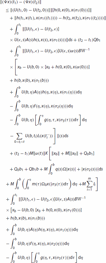
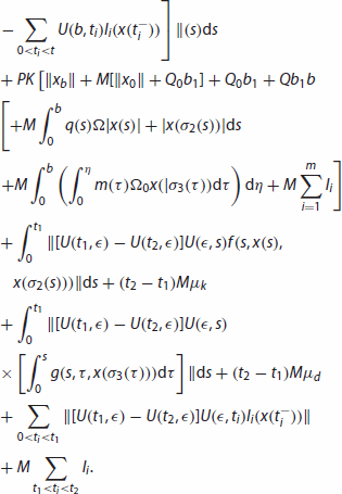
From the system (8), (i)–(v) and (H1)–(H9), we have $\begin{array}{rl}\parallel x\left(t\right)\parallel & \le M[\parallel x_0\parallel +|Q_0{b}_1]+Q_0{b}_1+Q{b}_{1}b\\ & +(bM\parallel \alpha (b)\parallel +P)K\left[\parallel x_b\parallel +M(\parallel x_0\parallel +Q_0{b}_1)\phantom{\sum _{i=1}^m{l}_i}\right.\\ & +Q_0{b}_1+Q{b}_{1}b+M{\int }_0^{b}q\left(s\right)\mathrm{\Omega }|x\left(s\right)|\\ & +|x\left({\sigma }_2\right(s\left)\right)|\mathrm{d}s\\ & +M{\int }_0^b\left({\int }_0^{\eta }m\left(\tau \right){\mathrm{\Omega }}_{0}x\left(|{\sigma }_3\right(\tau \left)\right)\mathrm{d}\tau \right)\mathrm{d}\eta \\ & \left.+M\sum _{i=1}^m{l}_i\right]+M{\int }_0^{t}q\left(s\right)\mathrm{\Omega }|x\left(s\right)|+|x\left({\sigma }_2\right(s\left)\right)|\mathrm{d}s\\ & +M{\int }_0^t\left({\int }_0^{s}m\left(\tau \right){\mathrm{\Omega }}_{0}x\left(|{\sigma }_3\right(\tau \left)\right)\mathrm{d}\tau \right)\mathrm{d}\eta \\ & +M\sum _{i=1}^m{l}_i.\\ & \le Q_1+Q_3+Q_{2}M{\int }_0^{b}q\left(\eta \right)\mathrm{\Omega }(2\parallel x\parallel )\mathrm{d}\eta \\ & +Q_{2}M{\int }_0^b\left[{\int }_0^{\eta }m\left(\tau \right){\mathrm{\Omega }}_0(\parallel x(\tau )\parallel ))\mathrm{d}\tau \right]\mathrm{d}\eta \\ & +M{\int }_0^{t}q\left(s\right)\mathrm{\Omega }(2\parallel x(s)\parallel )\mathrm{d}s\\ & +M{\int }_0^t\left[{\int }_0^{s}m\left(\tau \right){\mathrm{\Omega }}_0(\parallel x(\tau )\parallel ))\mathrm{d}\tau \right]\mathrm{d}s.\end{array}$ Let us take the right side of the above inequality as $\mu \left(t\right).$ Then, we have $\begin{array}{rl}x\left(t\right)& \le \mu \left(t\right),0\le t\le b,\\ a^{\ast }=\mu \left(0\right)& =Q_1+Q_3+Q_{2}M{\int }_0^{b}q\left(\eta \right)\mathrm{\Omega }(2\parallel x\parallel )\mathrm{d}\eta \\ & +Q_{2}M{\int }_0^b\left[{\int }_0^{\eta }m\right(\tau \left){\mathrm{\Omega }}_0\right(\parallel x\left(\tau \right)\parallel \left)\right)\mathrm{d}\tau ]\mathrm{d}\eta \\ {\mu }^{\mathrm{\prime }}\left(t\right)& =Mq\left(t\right)\mathrm{\Omega }2\parallel x\left(t\right)\parallel +M{\int }_0^{t}m\left(s\right){\mathrm{\Omega }}_0\parallel x\left(s\right)\parallel \mathrm{d}s\\ & \le Mq\left(t\right)\mathrm{\Omega }2\left(\mu \right(t\left)\right)+M{\int }_0^{t}m\left(s\right){\mathrm{\Omega }}_0\left(\mu \right(s\left)\right)\mathrm{d}s.\end{array}$ $Letw\left(t\right)=\mu \left(t\right)+{\int }_0^{t}m\left(s\right){\mathrm{\Omega }}_0\mu \left(s\right)\mathrm{d}s$. Then, $w\left(0\right)=\mu \left(0\right),\mu \left(t\right)\le w\left(t\right)\text{and}$ $\begin{array}{rl}{w}^{\mathrm{\prime }}\left(t\right)& ={\mu }^{\mathrm{\prime }}\left(t\right)+m\left(t\right){\mathrm{\Omega }}_0\mu \left(t\right)\\ & \le Mq\left(t\right)\mathrm{\Omega }2\left(w\right(t\left)\right)+m\left(t\right){\mathrm{\Omega }}_0\left(w\right(t\left)\right)\\ & \le p\left(t\right)\left[\mathrm{\Omega }2\right(w\left(t\right))+{\mathrm{\Omega }}_0(w\left(t\right)\left)\right].\end{array}$ This implies $\begin{array}{rl}{\int }_{w\left(0\right)}^{w\left(t\right)}\frac{\mathrm{d}s}{2\mathrm{\Omega }\left(s\right)+{\mathrm{\Omega }}_0\left(s\right)}& \le {\int }_0^b\hat{p}\left(s\right)\mathrm{d}s\\ & <{\int }_{a^{\ast }}^{\mathrm{\infty }}\frac{\mathrm{d}s}{2\mathrm{\Omega }\left(s\right)+{\mathrm{\Omega }}_0\left(s\right)}.\end{array}$

This inequality implies that there exists a constant $\mathcal{K}$ such that $w\left(t\right)\le \mathcal{K},t\in J$ and hence we have $\parallel x\parallel =sup\left\{|x\right(t)|:t\in J\}\le \mathcal{K}$ where $\mathcal{K}$ depends only on b and the functions $m,\mathrm{\Omega }$ and ${\mathrm{\Omega }}_0.$

Therefore it follows from the Schaefer fixed-point theorem that the operator Ψ has a fixed point $x\in {\mathbb{B}}_k$. Hence, the system (2(2) $\begin{array}{rl}& \frac{\mathrm{d}}{\mathrm{d}t}\left[x\right(t)+h(t,x\left(t\right),x\left({\sigma }_1\right(t\left)\right)]\\ & =\alpha \left(t\right)x\left(t\right)+f(t,x(t),x({\sigma }_2\left(t\right)\left)\right)\\ & +{\int }_0^{t}g(t,s,x({\sigma }_3\left(s\right)\left)\right)\mathrm{d}s,t\ne t_i,t\in J=[0,b],\\ & x\left(0\right)=x_0,\\ & \theta x\left(t\right)=B_{1}u\left(t\right),t\in J=[0,b],\\ & \mathrm{\Delta }x{|}_{t=t_i}=I_i\left(x\right(t_i^{-}\left)\right),i=1,2,\dots m,\end{array}$(2) ) is controllable on J.

5. Example

Consider the following boundary control integrodifferential evolution system: (9) $\begin{array}{rl}& \frac{\mathrm{\partial }}{\mathrm{\partial }t}\left[z\right(t,y)+h(t,z(t,y)\left)\right]\\ & =a(t,y)\frac{{\mathrm{\partial }}^2}{\mathrm{\partial }{y}^2}z(t,y)+a_1(t,z(t,y\left)\right)\\ & +{\int }_0^t{a}_2(t,s,z(t,y\left)\right)\mathrm{d}s,0\le y\le \pi ,t\in J=[0,b],\end{array}$(9) (10) $z(t,x)=u(t,x)\text{on}\mathrm{\Sigma }=(0,b)\times \mathrm{\Gamma },$(10) (11) $z(t,0)=z(t,\pi )=0,t\ge 0,$(11) (12) $z(0,y)=z_0\left(y\right),$(12) (13) $\begin{array}{rl}\mathrm{\Delta }z{|}_{t=t_i}=I_i\left(z\right(y\left)\right)& =\left({\gamma }_i|z\right(y)|+t_i{)}^{-1},\\ & z\in \mathbb{X},1\le i\le m,\end{array}$(13) where $a(t,y)$ is continuous on $0\le y\le \pi ,0\le t\le b$ and the constant ${\gamma }_i$ is small. Let us take $\mathbb{X}=U={\mathcal{L}}^2[0,\pi ]$ endowed with the usual norm $|\cdot {|}_{{\mathcal{L}}^2}.$ Put $x\left(t\right)=z(t,y).$

Define the operators $h,f,g,I_i$ by $\begin{array}{rl}h(t,\psi )\left(y\right)& =h(t,\psi (t,y\left)\right),\\ f(t,\psi )\left(y\right)& =a_1(t,\psi (t,y\left)\right),\\ g(t,\psi )\left(y\right)& ={\int }_0^t{a}_2(t,s,\psi (t,y\left)\right)\mathrm{d}s,\\ I_i\left(\psi \right)\left(y\right)& =\left({\gamma }_i|\psi \right(y)|+t_i{)}^{-1}.\end{array}$ In particular, set $\mathbb{X}={\mathbb{R}}^{+},J=[0,1]$ $\begin{array}{rl}f(t,x)& =\frac{1}{(1+t{)}^2}\frac{x\left(t\right)}{1+x\left(t\right)}+\frac{1}{16}v\left(t\right),\\ g(t,s,x)& ={\int }_0^t{\mathrm{e}}^{\left(-1/4\right)x\left(s\right)},\mathrm{d}s\\ h(t,x)& =\frac{{\mathrm{e}}^{-}t}{7+{\mathrm{e}}^t}\frac{x\left(t\right)}{1+x\left(t\right)}+\frac{1}{8}v\left(t\right),\\ I_i\left(x\right)& =\frac{1}{9}\cos x.\end{array}$ Let $x,y\in \mathbb{X}.$ Then, we have $\begin{array}{rl}\parallel f(t,x)-f(t,y)\parallel & \le \frac{1}{(t+4{)}^2}\frac{\parallel x-y\parallel }{(1+\parallel x\parallel )(1+\parallel y\parallel )}\\ & +\frac{1}{16}\parallel v-w\parallel \\ & \le \frac{1}{(t+4{)}^2}\parallel x-y\parallel +\frac{1}{16}\parallel v-w\parallel \\ & \le \frac{1}{16}[\parallel x-y\parallel +\parallel v-w\parallel ].\end{array}$ Hence, the condition (H5) holds with $K_f=\frac{1}{16}.$Let $x,y\in \mathbb{X}.$ Then, we have $\begin{array}{rl}& \parallel g(t,x)-g(t,y)\parallel \\ & =∥{\int }_0^t{\mathrm{e}}^{\left(-1/4\right)x\left(s\right)}\mathrm{d}s-{\int }_0^t{\mathrm{e}}^{\left(-1/4\right)y\left(s\right)}\mathrm{d}s∥\\ & \le \frac{1}{4}\parallel x-y\parallel .\end{array}$ Hence, the condition (H6) holds with $N_g=\frac{1}{4}.$Let $x,y\in \mathbb{X}.$ Then, we have $\begin{array}{rl}\parallel h(t,x)-h(t,y)\parallel & =\frac{{\mathrm{e}}^{-}t}{7+{\mathrm{e}}^t}∥\frac{x\left(t\right)}{1+x\left(t\right)}-\frac{y\left(t\right)}{1+y\left(t\right)}∥\\ & +\frac{1}{8}\parallel v-w\parallel \\ & \le \frac{{\mathrm{e}}^{-}t}{7+{\mathrm{e}}^t}\parallel x-y\parallel +\frac{1}{8}\parallel v-w\parallel \\ & \le \frac{1}{8}[\parallel x-y\parallel +\parallel v-w\parallel ].\end{array}$ Hence, the condition (H4) holds with $L_1=\frac{1}{8}.$Let $x,y\in \mathbb{X}.$ Then, we have $\begin{array}{rl}\parallel I_i\left(x\right)-I_i\left(y\right)\parallel & =\parallel \frac{1}{9}\cos x-\frac{1}{9}cosy\parallel \\ & \le \frac{1}{9}\parallel x-y\parallel .\end{array}$ Hence, the condition (H3) holds with $l_i=\frac{1}{9}.$Assume that the linear operator $\mathbb{W}$ from ${\mathcal{L}}^2(J,\mathbb{Y})/ker\mathbb{W}$ into $\mathbb{X}$ defined by $\mathbb{W}u={\int }_0^b\left[U\right(b,s\left)\alpha \right(s)-U(b,s\left)A\right(s\left)\right]Bu\left(s\right)\mathrm{d}s$ induces an invertible operator ${\mathbb{W}}^{-1}$ on ${\mathcal{L}}^2(J,\mathbb{Y})/ker\mathbb{W}$.

Choose K=1 in such a way that $\mathrm{\Lambda }=M{L}_1+\widetilde{M_0}+(Mb\parallel \alpha (b)\parallel +P)K(M{L}_1+\widetilde{M_0})<1$,where $\widetilde{M_0}=0.3611,$ which is satisfied for some $q\in [0,1].$ All the remaining conditions of Theorem (3.1) are satisfied. Hence, the system (9(9) $\begin{array}{rl}& \frac{\mathrm{\partial }}{\mathrm{\partial }t}\left[z\right(t,y)+h(t,z(t,y)\left)\right]\\ & =a(t,y)\frac{{\mathrm{\partial }}^2}{\mathrm{\partial }{y}^2}z(t,y)+a_1(t,z(t,y\left)\right)\\ & +{\int }_0^t{a}_2(t,s,z(t,y\left)\right)\mathrm{d}s,0\le y\le \pi ,t\in J=[0,b],\end{array}$(9) )–(13(13) $\begin{array}{rl}\mathrm{\Delta }z{|}_{t=t_i}=I_i\left(z\right(y\left)\right)& =\left({\gamma }_i|z\right(y)|+t_i{)}^{-1},\\ & z\in \mathbb{X},1\le i\le m,\end{array}$(13) ) is controllable on J.

6. Conclusion

To summarize this, authors investigated the boundary controllability results for neutral impulsive integrodifferential evolution systems with time-varying delay in Banach spaces by semigroup theory and the evolution operator. Also proved that the existence and uniqueness of first-order impulsive integrodifferential evolution system by using $C_0$-semigroup and the Banach contraction principle and thereby shown that the governing system is controllable. Furthermore, based on Schaefer's fixed point theorem, sufficient conditions of controllability for the given system have been obtained by using analytic semigroup. Finally provide an example to illustrate the theory.

7. Future research

Current investigation of the neutral impulsive integrodifferential evolution systems with time-varying delays gives an analytical result only. In future, this work will be implemented to find the numerical solutions also. Moreover, recently fractional differential equations are increasingly used for many mathematical models in science and engineering. Fractional differential equations have attracted considerable interest because of their ability to model complex phenomena. It is also serve as an excellent tool for the description of hereditary properties of various materials and processes. In fact, fractional differential equations are considered as an alternative model to non-linear differential equation. So the current work extended under fractional differential equations too.

Acknowledgements

The authors are grateful to an anonymous referee for valuable comments and suggestions, which helped to improve the quality of the paper.

Disclosure statement

No potential conflict of interest was reported by the authors.

ORCID

B. Radhakrishnan  http://orcid.org/0000-0002-0451-5525

P. Chandru  http://orcid.org/0000-0002-2652-1723

References

- Pazy A. Semigroups of linear operators and applications to partial differential equations. New York: Springer-Verlag; 1983.
- Balachandran K, Dauer JP. Controllability of nonlinear systems in Banach spaces: a survey. J Optim Theory Appl. 2002;115:7–28. doi: 10.1023/A:1019668728098
- Radhakrishnan B, Balachandran K. Controllability results for nonlinear impulsive integrodifferential evolution systems with time-varying delays. J Control Theory Appl. 2013;11:415–421. doi: 10.1007/s11768-013-2147-2
- Radhakrishnan B, Balachandran K. Controllability of impulsive neutral functional evolution integrodifferential systems with infinite delay. Nonlinear Anal Hybrid Syst. 2011;5:655–670. doi: 10.1016/j.nahs.2011.05.001
- Radhakrishnan B, Balachandran K. Controllability results for second order neutral impulsive integrodifferential systems. J Optim Theory Appl. 2011;151:589–612. doi: 10.1007/s10957-011-9860-0
- Hernandez E, Henriquez HR. Existence results for partial neutral functional differential equations with unbounded delay. J Math Anal Appl. 1998;221:452–475. doi: 10.1006/jmaa.1997.5875
- Lakshmikantham V, Bainov DD, Simeonov PS. Theory of impulsive differential equations. Singapore: World Scientific; 1989.
- Samoilenko AM, Perestyuk NA. Impulsive differential equations. Singapore: World Scientific; 1995.
- Hernandez E, Henriquez HR. Impulsive partial neutral differential equations. Appl Math Lett. 2006;19:215–222. doi: 10.1016/j.aml.2005.04.005
- Balachandran K, Kim JH, Leelamani A. Existence results for nonlinear abstract neutral differential equations with time varying delays. Appl Math E-Notes. 2006;6:186–193.
- Balakrishnan AV. Applied functional analysis. New York: Springer-Verlag; 1976.
- Curtain RF, Zwart H. An introduction to infinite dimensional linear systems theory. New York: Springer-Verlag; 1995.
- Fattorini HO. Boundary control systems. SIAM J Control. 1968;6:349–384. doi: 10.1137/0306025
- Washburn D. A bound on the boundary input map for parabolic equation with application to time optimal control. SIAM J Control Optim. 1979;17:652–671. doi: 10.1137/0317046
- Barbu V. Boundary control problems with convex cost criterion. SIAM J Control Optim. 1980;18:227–243. doi: 10.1137/0318016
- Balachandran K, Anandhi ER. Boundary controllability of integrodifferential systems in Banach spaces. Proc Indian Acad Sci (Math Sci). 2001;111:127–135. doi: 10.1007/BF02829544
- Balachandran K, Anandhi ER. Boundary controllability of neutral integrodifferential systems in Banach spaces. Nihonkai Math J. 2004;15:1–13.
- Liu JH. Nonlinear impulsive evolution equations. Dyn Contin Discrete Impul Syst. 1999;6:77–85.
- Gorniewicz L, Ntouyas SK, O'Regan D. Controllability of semilinear differential equations and inclusions via semigroup theory in Banach spaces. Rep Math Phys. 2005;56:437–470. doi: 10.1016/S0034-4877(05)80096-5
- Schaefer H. Uber die methode der a priori schranken. Math Annalem. 1995;129:415–416. doi: 10.1007/BF01362380