Peristaltic transport of a power-law fluid in an elastic tube

ABSTRACT

A mathematical model is proposed to study the influence of elasticity on the peristaltic flow of a generalized Newtonian fluid in a tube. A power-law model is considered in the present study to understand the effect of elasticity on the peristaltic flow of blood through arteries. Application of blood flow through arteries is studied by expressing a relationship between pressure gradient and volume flow rate in an elastic tube. The results show the significant effect of elasticity on flow quantities. It is observed that the flux increases as the fluid behaviour index increases and that the flux is more for a Newtonian fluid when compared to non-Newtonian cases. The trapping phenomenon is presented graphically for various physical parameters. The results obtained in the present study are compared with an earlier investigation of Vajravelu et al. (Peristaltic transport of a Herschel–Bulkley fluid in an elastic tube. Heat Transf-Asian Res. 2014;44:585–598).

KEYWORDS:

• Elastic tube
• peristaltic flow
• non-Newtonian fluid
• power-law index
• volume flow rate

Nomenclature

$b$	=	Amplitude of the wave
$\phi$	=	Amplitude ratio
$\theta$	=	Azimuthal angle
${\alpha }^{\mathrm{\prime }}$	=	Change in the radius of the tube due to peristalsis
${\alpha }^{\mathrm{\prime \prime }}$	=	Change in the radius of the tube due to elasticity
${\overline{\tau }}_{ij}$	=	Components of extra stress tensor in stationary frame
$\sigma$	=	Conductivity
$z$	=	Distance along the tube from inlet end
$\rho$	=	Density
$\overline{q}$	=	Dimensional flux in fixed frame
$F$	=	Dimensionless flux in moving frame
$t_1,t_2$	=	Elastic parameters
$p_e$	=	External pressure
$p_i$	=	Inlet pressure
$L$	=	Length of the tube
$(\overline{r},\overline{w})$	=	Moving coordinates
$p_o$	=	Outlet pressure
$n$	=	Power-law Index
$p\left(z\right)$	=	Pressure of the fluid
$P$	=	Pressure gradient
${\alpha }_0$	=	Radius of the tube in the absence of elasticity
$(\overline{R},\overline{Z})$	=	Stationary coordinates
${\dot{\gamma }}_{ij}$	=	Strain-rate tensor
$\psi$	=	Stream function
$T$	=	Tension of the tube wall
$t$	=	Time
$(\overline{w},\overline{u})$	=	Velocity components in moving frame
$(\overline{W},\overline{U})$	=	Velocity components in stationary frame
$\lambda$	=	Wavelength of the peristaltic wave
$\delta$	=	Wave number
$c$	=	Wave speed
$K$	=	Constant

1. Introduction

The present study analyses the effect of elastic properties on the peristaltic flow of a generalized Newtonian fluid in a tube. Many fluid models can be encountered in the literature and those models found extensive use in the analysis of the flow behaviour of Newtonian and non-Newtonian fluids. In particular, the study of blood flow in arteries is modelled by non-Newtonian fluids, in which the stress and strain-rate relation is non-linear. In the present study, the flow of a power-law fluid is considered under the long wave length and low Reynolds number approximations to understand both peristaltic and elasticity effects. Peristalsis is an inherent property in many biological systems which are elastic in nature; so it is important to study the peristaltic flow characteristics of a power-law fluid in an elastic tube.

Different models were proposed by various investigators to study the peristaltic mechanism in physiological situations by considering the Newtonian or non-Newtonian fluids. But most of the research works are concentrated on fluid flow though rigid tubes/channels. To understand the rheological properties of physiological fluids in living organisms, the elastic nature of flow geometries is taken into consideration. For example, blood flow in the tissue is different from the blood flow in a microvasculature of the tissue. Since microvasculature flow rates vary in pathological conditions when compared to normal conditions, it is important to study the consequences of blood flow through small arteries which are having elastic properties.

Fluid flow through flexible tubes is of interest due to its dynamic similarity to that of fluid flow in veins, arteries, urethra and so on. The significant application of elastic tubes involves modelling elastic deformation of hallow tubes, mechanical evaluation of elastic tubes used in physical therapy, cardiovascular systems to understand the evolution of pathology due to vessel deformation, and diagnostic and therapeutic devices such as pressurized cuffs and prosthetic heart devices.

In literature, a number of theoretical and experimental studies are available on the peristaltic flow mechanism for different fluids with different flow geometries. Shapiro et al. [1] examined pumping by means of a peristaltic wave under long wavelength and low Reynolds number approximations. A relationship between pressure rise per wavelength and time mean flow is derived. The results are compared with experimental data using a quasi two-dimensional apparatus. Radhakrishnamacharya [2] analysed the peristaltic motion of a power-law fluid using asymptotic expansion in terms of a slope parameter. Shukla et al. [3] studied the effect of a peripheral layer and variable consistency on the peristaltic flow characteristics of a power-law fluid in a tube. Srivastava and Srivastava [4] discussed the peristaltic transport of a power-law fluid in a uniform and non-uniform channel. Rao and Mishra [5] considered the axis symmetric porous tube to investigate the trapping and reflux phenomenon for the peristaltic flow of a power-law fluid. The helical flow of a power-law fluid in a thin annulus with permeable walls is studied by Vajravelu et al. [6]. The mechanism of a power-law fluid with peristalsis is analysed by Hayat and Ali [7]. The hydrodynamic flow of a generalized Newtonian fluid through a uniform tube with peristalsis is studied by Naby et al. [8]. The MHD effects on the peristaltic mechanism through a porous space and the influence of heat and mass transfer is presented by Srinivas and Kothandapani [9].

A number of investigations on the rheology of blood through arteries are found in earlier studies by taking the elastic property into consideration. Roach and Burton [10] conducted an experiment on the human external iliac artery to study the static pressure–volume relation as tension versus length curve and explained the reasons for distensibility of the shape of arteries. Whirlow and Rouleau [11] proposed a model to explain the arterial blood flow using a thick-walled viscoelastic tube consisting of a viscous fluid. A non-linear analysis of flow in an elastic tube is discussed by Wang and Tarbell [12]. Sankara and Jayaraman [13] considered the annulus of an elastic tube to study the application to a catheterized artery with a non-linear analysis of oscillatory flow. Johnston et al. [14] studied the blood flow through arteries by considering five different types of non-Newtonian fluids in four different right coronary arteries and concluded that the generalized power-law model gives better approximations of wall shear stress at low shear. Modelling and analysis of blood flow in elastic arteries are explained by Sharma et al. [15]. Pandey and Chaube [16] considered the flexible tube of changing cross-section to study the Maxwell fluid flow characteristics with peristalsis. Takaghi and Balmforth [17] applied a lubrication analysis to model the deformation of the tube wall and determined the pumping efficiency.

Vajravelu et al. [18] considered the case of inserting a catheter into an elastic tube to observe the changes in the blood flow pattern by taking a Herschel–Bulkley fluid. Sochi [19] proposed the expression for the volumetric flow as a function pressure in an elastic tube using two pressure-area constitutive relations. The effect of peristalsis on the Herschel–Bulkley fluid flow in an elastic tube was discussed by Vajravelu et al. [20]. Chaube et al. [21] analysed the peristaltic creeping flow of power-law physiological fluids through a non-uniform channel with slip effects. Ali et al. [22] investigated the numerical simulation on the peristaltic flow of a biorheological fluid with a shear-dependent viscosity in a curved channel. Further, Vajravelu et al. [23] analysed the peristaltic transport of a Casson fluid in an elastic tube.

Numerical simulation of heat transfer in blood flow altered by electro-osmosis through tapered micro-vessels is analysed by Prakash et al. [24]. A study on the electro osmotic flow of biorheological micropolar fluids through microfluidic channels is presented by Chaube et al. [25]. Prakash and Tripathi [26] discussed the electro osmotic flow of Williamson ionic nanoliquids in a tapered microfluidic channel in the presence of thermal radiation and peristalsis. Thermally developed peristaltic propulsion of magnetic solid particles in biorheological fluids is studied by Batti et al. [27]. Electro-osmosis-modulated peristaltic biorheological flow through an asymmetric micro-channel is investigated by Tripathi et al. [28]. Further, Tripathi et al. [29] examined the computer modelling of electro-osmotically augmented three-layered micro-vascular peristaltic blood flow.

Motivated by the earlier studies, it is important to consider the elastic nature of the tube to understand the blood rheology in physiological systems. The present problem is to study the effects of elasticity on a power-law fluid flow through a tube with peristalsis. The problem is modelled under the assumptions that the tube length is an integral multiple of wavelength and flow to be of inertia free. The analytic expressions are derived for flow quantities and results are analysed through graphs.

2. Mathematical formulation

Figure 1 represents the peristaltic flow of a steady incompressible power-law fluid in an elastic tube of length $L$ and radius $\alpha \left(z\right)$. The tube walls are subjected to an infinite sinusoidal wave movement with the constant speed $c$. At any axial station $z$, the instantaneous radius of the tube is given by (1) $\overline{R}={\overline{\alpha }}^{\mathrm{\prime }}(\overline{z},\overline{t})={\alpha }_0+b\sin \frac{2\pi }{\lambda }(\overline{Z}-c\overline{t}),$(1) where ${\alpha }_0$ is the radius of the tube in the absence of elasticity, $b$ the amplitude of the peristaltic wave and $\overline{t}$ is the time. We choose the cylindrical coordinate system $(\overline{R},\theta ,\overline{Z})$ , where $\overline{Z}$-axis lies along the centre line of the tube and $\overline{R}$ is the radius of the tube. The flow is unsteady in the lab frame and it becomes steady in the wave frame. The transformation between stationary coordinates $(\overline{R},\overline{Z})$ and moving coordinates $(\overline{r},\overline{z})$ is given by (2) $\overline{z}=\overline{Z}-c\overline{t};\overline{r}=\overline{R};\overline{w}=\overline{W}-c;\overline{u}=\overline{U}.$(2) Here, $\overline{U}\text{and}\overline{W}$ are the radial and axial velocity components in fixed coordinates. $\overline{u}\text{and}\overline{w}$ are the radial and axial velocity components in moving coordinates.

Figure 1. Physical model.

The continuity equation and equations of motion in the wave frame are given by (3) $\frac{1}{\overline{r}}\frac{\mathrm{\partial }\left(\overline{ru}\right)}{\mathrm{\partial }\overline{r}}+\frac{\mathrm{\partial }\overline{w}}{\mathrm{\partial }\overline{z}}=0,$(3) (4) $\rho \left(\overline{u}\frac{\mathrm{\partial }\overline{u}}{\mathrm{\partial }\overline{r}}+\overline{w}\frac{\mathrm{\partial }\overline{u}}{\mathrm{\partial }\overline{z}}\right)=-\frac{\mathrm{\partial }\overline{p}}{\mathrm{\partial }\overline{r}}-\left[\frac{1}{\overline{r}}\frac{\mathrm{\partial }\left(\overline{r}{\overline{\tau }}_{11}\right)}{\mathrm{\partial }\overline{r}}+\frac{\mathrm{\partial }{\overline{\tau }}_{31}}{\mathrm{\partial }\overline{z}}-\frac{{\overline{\tau }}_{22}}{\overline{r}}\right],$(4) (5) $\rho \left(\overline{u}\frac{\mathrm{\partial }\overline{w}}{\mathrm{\partial }\overline{r}}+\overline{w}\frac{\mathrm{\partial }\overline{w}}{\mathrm{\partial }\overline{z}}\right)=-\frac{\mathrm{\partial }\overline{p}}{\mathrm{\partial }\overline{z}}-\left[\frac{1}{\overline{r}}\frac{\mathrm{\partial }\left(\overline{r}{\overline{\tau }}_{13}\right)}{\mathrm{\partial }\overline{r}}+\frac{\mathrm{\partial }{\overline{\tau }}_{33}}{\mathrm{\partial }\overline{z}}\right].$(5)

The constitutive equation for an Ostwald-de Waele power-law fluid can be expressed by Bird et al. [30] as (6) ${\overline{\tau }}_{ij}=-m(\overline{\dot{\gamma }}{)}^{n-1}{\overline{\dot{\gamma }}}_{ij},$(6) where ${\overline{\tau }}_{ij},i,j=1,2,3$ are components of the extra stress tensor, $m$ is the consistency parameter, $n$ is the fluid behaviour index and $\overline{\dot{\gamma }}$ is defined as (7) $\overline{\dot{\gamma }}=\sqrt{\frac{1}{2}\sum _i\sum _j{\overline{\dot{\gamma }}}_{ij}{\overline{\dot{\gamma }}}_{ij}}=\sqrt{\frac{1}{2}{\mathrm{\Gamma }}_{{\overline{\dot{\gamma }}}_{ij}}},$(7) where ${\mathrm{\Gamma }}_{\overline{\dot{\gamma }}}$ is the second invariant of strain-rate tensor ${\overline{\dot{\gamma }}}_{ij}$.

The rate of strain tensor ${\overline{\dot{\gamma }}}_{ij}$ has the following components: (8) $\begin{array}{rl}{\overline{\dot{\gamma }}}_{11}& =2\frac{\mathrm{\partial }\overline{u}}{\mathrm{\partial }\overline{r}},{\overline{\dot{\gamma }}}_{22}=2\frac{\overline{u}}{\overline{r}},{\overline{\dot{\gamma }}}_{33}=2\frac{\mathrm{\partial }\overline{w}}{\mathrm{\partial }\overline{z}},\text{ and }\\ {\overline{\dot{\gamma }}}_{13}& ={\overline{\dot{\gamma }}}_{31}=\frac{\mathrm{\partial }\overline{u}}{\mathrm{\partial }\overline{z}}+\frac{\mathrm{\partial }\overline{w}}{\mathrm{\partial }\overline{r}},\end{array}$(8) and corresponding boundary conditions are (9) $\frac{\mathrm{\partial }\overline{w}}{\mathrm{\partial }\overline{r}}=0\text{at }\overline{r}=0,$(9) (10) $\overline{w}=-c\text{at }\overline{r}={\overline{\alpha }}^{\mathrm{\prime }}.$(10) Introducing the non-dimensional quantities, (11) $\begin{array}{r}\begin{array}{rl}z& =\frac{\overline{z}}{\lambda },\text{Z}=\frac{\overline{Z}}{\lambda },R=\frac{\overline{R}}{{\alpha }_0}r=\frac{\overline{r}}{{\alpha }_0},U=\frac{\lambda \overline{U}}{{\alpha }_{0}c},u=\frac{\lambda \overline{u}}{{\alpha }_{0}c},\\ W& =\frac{\overline{W}}{c},w=\frac{\overline{w}}{c},t=\frac{c\overline{t}}{\lambda },p=\frac{{{\alpha }_0}^{n+1}\overline{p}}{c^{n}m\lambda },\\ \text{Re}& =\frac{\rho {{\alpha }_0}^n}{c^{n-2}m},\phi =\frac{b}{{\alpha }_0},\\ \delta & =\frac{{\alpha }_0}{\lambda },{\alpha }^{\mathrm{\prime }}=\frac{{\overline{\alpha }}^{\mathrm{\prime }}}{{\alpha }_0},{\alpha }^{\mathrm{\prime \prime }}=\frac{{\overline{\alpha }}^{\mathrm{\prime \prime }}}{{\alpha }_0},F=\frac{\overline{q}}{\pi {\alpha }_0^{2}c},\dot{\gamma }=\frac{{\alpha }_0\overline{\dot{\gamma }}}{c},\\ {\tau }_{ij}& =\frac{{{\alpha }_0}^n{\overline{\tau }}_{ij}}{c^{n}m}\text{for}i\ne j,{\tau }_{ij}=\frac{\lambda {{\alpha }_0}^{n-1}{\overline{\tau }}_{ij}}{c^{n}m}\text{for}i=j,\\ {\dot{\gamma }}_{ij}& =\frac{{\alpha }_0{\overline{\dot{\gamma }}}_{ij}}{c}\text{for}i\ne j,{\dot{\gamma }}_{ij}=\frac{\lambda {\overline{\dot{\gamma }}}_{ij}}{c}\text{for}i=j.\end{array}\end{array}$(11) Equations (3)–(5) in non-dimensional form are given by (12) $\frac{1}{r}\frac{\mathrm{\partial }\left(ru\right)}{\mathrm{\partial }r}+\frac{\mathrm{\partial }w}{\mathrm{\partial }z}=0,$(12) (13) $\begin{array}{rl}& \text{Re}{\delta }^3\left(u\frac{\mathrm{\partial }u}{\mathrm{\partial }r}+w\frac{\mathrm{\partial }u}{\mathrm{\partial }z}\right)=-\frac{\mathrm{\partial }p}{\mathrm{\partial }r}\\ & -\left[{\delta }^2\frac{1}{r}\frac{\mathrm{\partial }\left(r{\tau }_{11}\right)}{\mathrm{\partial }r}+{\delta }^2\frac{\mathrm{\partial }{\tau }_{31}}{\mathrm{\partial }z}-{\delta }^2\frac{{\tau }_{22}}{r}\right],\end{array}$(13) (14) $\text{Re}\delta \left(u\frac{\mathrm{\partial }w}{\mathrm{\partial }r}+w\frac{\mathrm{\partial }w}{\mathrm{\partial }z}\right)=-\frac{\mathrm{\partial }p}{\mathrm{\partial }z}-\left[\frac{1}{r}\frac{\mathrm{\partial }\left(r{\tau }_{13}\right)}{\mathrm{\partial }r}+{\delta }^2\frac{\mathrm{\partial }{\tau }_{33}}{\mathrm{\partial }z}\right].$(14)

The dimensionless boundary conditions are (15) $\frac{\mathrm{\partial }w}{\mathrm{\partial }r}=0\text{at }r=0,$(15) (16) $w=-1\text{at }r={\alpha }^{\mathrm{\prime }}.$(16) Equations (6)–(8) in non-dimensional form are (17) ${\tau }_{ij}=-(\dot{\gamma }{)}^{n-1}{\dot{\gamma }}_{ij},$(17) $\dot{\gamma }=\sqrt{\frac{1}{2}{\delta }^2\sum _i\sum _j{\dot{\gamma }}_{ij}{\dot{\gamma }}_{ij}},\text{ for }i=j,$ (18) $\dot{\gamma }=\sqrt{\frac{1}{2}\sum _i\sum _j{\dot{\gamma }}_{ij}{\dot{\gamma }}_{ij}},\text{ for }i\ne j,$(18) (19) $\begin{array}{rl}{\dot{\gamma }}_{11}& =2\frac{\mathrm{\partial }u}{\mathrm{\partial }r},{\dot{\gamma }}_{22}=\frac{2u}{r},{\dot{\gamma }}_{33}=2\frac{\mathrm{\partial }w}{\mathrm{\partial }z},\\ {\dot{\gamma }}_{13}& ={\dot{\gamma }}_{31}={\delta }^2\frac{\mathrm{\partial }u}{\mathrm{\partial }z}+\frac{\mathrm{\partial }w}{\mathrm{\partial }r}.\end{array}$(19) Neglecting the wave number $\delta$, Equations (12)–(14) reduces to (20) $\frac{1}{r}\frac{\mathrm{\partial }\left(ru\right)}{\mathrm{\partial }r}+\frac{\mathrm{\partial }w}{\mathrm{\partial }z}=0,$(20) (21) $\frac{\mathrm{\partial }p}{\mathrm{\partial }r}=0,$(21) (22) $\frac{\mathrm{\partial }p}{\mathrm{\partial }z}=-\left[\frac{1}{r}\frac{\mathrm{\partial }\left(r{\tau }_{13}\right)}{\mathrm{\partial }r}\right].$(22) Substituting Equations (18) and (19) in Equation (17) results (23) ${\tau }_{13}={\left(-\frac{\mathrm{\partial }w}{\mathrm{\partial }r}\right)}^n.$(23) From Equation (22) and (23), we get (24) $\frac{\mathrm{\partial }p}{\mathrm{\partial }z}=-\frac{1}{r}\frac{\mathrm{\partial }}{\mathrm{\partial }r}\left[r{\left(-\frac{\mathrm{\partial }w}{\mathrm{\partial }r}\right)}^n\right],$(24)

3. Solution of the problem

Solving Equation (24) subject to the boundary conditions (15) and (16), we have (25) $w=-\frac{n}{n+1}{\left(-\frac{1}{2}\frac{\mathrm{\partial }p}{\mathrm{\partial }z}\right)}^{\frac{1}{n}}\left[r^{\frac{n+1}{n}}-{{\alpha }^{\mathrm{\prime }}}^{\frac{n+1}{n}}\right]-1;$(25) from Equation (25), the expression for stream function $\left(w=\frac{1}{r}\left(\frac{\mathrm{\partial }\psi }{\mathrm{\partial }r}\right),u=-\frac{1}{r}\left(\frac{\mathrm{\partial }\psi }{\mathrm{\partial }z}\right)\right)$ is obtained using the condition $\psi =0atr=0$ as (26) $\psi =-\frac{r^2}{2}-\frac{n}{n+1}{\left(-\frac{1}{2}\frac{dp}{dz}\right)}^{\frac{1}{n}}\left[\frac{n}{3n+1}{r}^{\frac{3n+1}{n}}-{{\alpha }^{\mathrm{\prime }}}^{\frac{3n+1}{n}}\right].$(26) The instantaneous volume flow rate $F$ through any cross-section is (27) $F=2\underset{0}{\overset{{\alpha }^{\mathrm{\prime }}}{\int }}rwdr.$(27) Substituting Equation (25) in Equation (27), we get (28) $F=\frac{n}{3n+1}{\left(\frac{1}{2}\right)}^{\frac{1}{n}}(P{)}^{\frac{1}{n}}{\alpha }^{\mathrm{\prime }\frac{3n+1}{n}}-{\alpha }^{\mathrm{\prime }2},$(28)

where $P=-\frac{dp}{dz}.$ Solving Equation (28) for $\frac{\text{d}p}{\text{d}z}$, we have (29) $\frac{\text{d}p}{\text{d}z}=\frac{-2{\left(\frac{3n+1}{n}\right)}^n{\left(F+{{\alpha }^{\mathrm{\prime }}}^2\right)}^n}{{{\alpha }^{\mathrm{\prime }}}^{3n+1}}.$(29)

4. Theoretical determination of flux – application to blood flow through artery

In this section, the elasticity of the tube wall is taken into consideration along with peristalsis to determine the variation of flux. Consider the peristaltic pumping of an incompressible power-law fluid through an elastic tube of length $L$ and radius $\alpha \left(z\right)$, as shown in Figure 1. Here, $\alpha \left(z\right)$ is the varying radius consisting of both peristalsis and elasticity effects. To calculate the flux of a power-law fluid through an elastic tube, we use the method of Rubinow and Keller [31]. Let $p_i$ and $p_o$ represent the pressure of fluid at the entrance and exit of the tube, respectively, and $p_e$ is the external pressure. Here, the inlet pressure $p_i$ is assumed to be greater than outlet pressure $p_o$. Also, the flux $F$ and the pressure gradient are related by the expression (30) $F=\sigma (p-p_e){\left(-\frac{\text{d}p}{\text{d}z}\right)}^{\frac{1}{n}}.$(30) Here, the proportionality factor $\sigma (p-p_e)$ is known as the conductivity of the tube. The conductivity of the tube depends on the shape of the cross-section of the tube, which is determined by pressure difference $p-p_e$ (Flaherty et al. [32]). As a result of inside and outside pressure difference, the tube wall may expand or contract. Due to this elastic property of the tube wall, there exist changes in the shape of cross-section of the tube. Hence, the conductivity $\sigma$ of the tube at $z$ depends on the pressure difference. Therefore, the conductivity $\sigma =\sigma \left[p\left(z\right)-p_e\right]$ is a function of $\left(p\right(z)-p_e)$.

From Equations (28) and (30), we have (31) $\sigma (p-p_e)=\frac{n}{(3n+1)2^{\frac{1}{n}}}{\alpha }^{\mathrm{\prime }\frac{1}{n}+3}.$(31) By taking elastic property into consideration in addition to the peristaltic movement, Equation (31) can be written as (32) $\sigma (p-p_e)=\frac{n}{(3n+1)2^{\frac{1}{n}}}({\alpha }^{\mathrm{\prime }}+{\alpha }^{\mathrm{\prime \prime }}{)}^{\frac{1}{n}+3}.$(32) Here ${\alpha }^{\mathrm{\prime }}\text{and }{\alpha }^{\mathrm{\prime \prime }}$ are the radius of the tube with peristalsis and elasticity, respectively. Since the flow is of Poiseuille type, the radius ${\alpha }^{\mathrm{\prime \prime }}$ is a function of $(p-p_e)$ at each cross-section. The tube wall deformation due to peristaltic wave is ${\alpha }^{\mathrm{\prime }}\left(z\right)=1+\phi \sin 2\pi z$.

Integrating Equation (30) with respect to $z$ from $z=0$ and applying inlet condition $p\left(0\right)=p_i$, we get (33) $\int \left\{F+{{\alpha }^{\mathrm{\prime }}}^2\right\}\text{d}z=K\underset{p\left(z\right)-p_e}{\overset{p_i-p_e}{\int }}\sigma \left(p^{\mathrm{\prime }}\right)\text{d}{p}^{\mathrm{\prime }},$(33) where $K=\frac{n}{(3n+1)2^{\frac{1}{n}}}.$ Here $p^{\mathrm{\prime }}=p\left(z\right)-p_e$. Equation (33) determines $p\left(z\right)$ implicitly in terms of $F$ and $z$. To find $F$, we set $z=1$ and $P\left(1\right)=p_o$ in Equation (33), which yields (34) $F+1+\frac{{\phi }^2}{2}-\frac{\phi }{\pi }=K\underset{p\left(1\right)-p_e}{\overset{p_i-p_e}{\int }}\sigma \left(p^{\mathrm{\prime }}\right)\text{d}{p}^{\mathrm{\prime }},$(34) (35) ${\left(F+1+\frac{{\phi }^2}{2}-\frac{\phi }{\pi }\right)}^n=K^n\underset{p\left(1\right)-p_e}{\overset{p_i-p_e}{\int }}{\left(\sigma \left(p^{\mathrm{\prime }}\right)\right)}^n\text{d}{p}^{\mathrm{\prime }};$(35) using Equation (32) in (35) (36) ${\left(F+1+\frac{{\phi }^2}{2}-\frac{\phi }{\pi }\right)}^n=K^n\underset{p_o-p_e}{\overset{p_i-p_e}{\int }}{\left({\alpha }^{\mathrm{\prime }}+{\alpha }^{\mathrm{\prime \prime }}\right)}^{3n+1}\text{d}{p}^{\mathrm{\prime }},$(36) We can evaluate Equation (36), if the function of the form ${\alpha }^{\mathrm{\prime \prime }}(p-p_e)$ is known.

If the tension in the tube wall $T\left({\alpha }^{\mathrm{\prime \prime }}\right)$ is a known function of ${\alpha }^{\mathrm{\prime \prime }}$, then ${\alpha }^{\mathrm{\prime \prime }}\left(p^{\mathrm{\prime }}\right)$ can be obtained from the equilibrium condition using Rubinow and Keller [31]. (37) $T\left({\alpha }^{\mathrm{\prime \prime }}\right)/{\alpha }^{\mathrm{\prime \prime }}=p-p_e.$(37)

5. Method of Rubinow and Keller

The static pressure–volume relation is determined by Roach and Burton [10], which is converted into a tension versus length curve. This relation is represented by the following equation using Rubinow and Keller [31]: (38) $T\left({\alpha }^{\mathrm{\prime \prime }}\right)=t_1({\alpha }^{\mathrm{\prime \prime }}-1)+t_2({\alpha }^{\mathrm{\prime \prime }}-1{)}^5,$(38) where $t_1=13$ and $t_2=300.$

Now, substituting Equations (37) in Equation (38), we have (39) $\begin{array}{rl}\text{d}{p}^{\mathrm{\prime }}& =\left[\frac{t_1}{{{\alpha }^{\mathrm{\prime \prime }}}^2}+t_2\left(4{{\alpha }^{\mathrm{\prime \prime }}}^3-15{{\alpha }^{\mathrm{\prime \prime }}}^2\right.\right.\\ & \left.\left.+20{\alpha }^{\mathrm{\prime \prime }}-10+\frac{1}{{{\alpha }^{\mathrm{\prime \prime }}}^2}\right)\right]\text{d}{\alpha }^{\mathrm{\prime \prime }}.\end{array}$(39) Substituting Equation (39) in (36), we evaluated the integral numerically from $p_o-p_e$ to $p_i-p_e$ using Mathematica software, and the flux is given as (40) $\begin{array}{rl}& {\left(F+1+\frac{{\phi }^2}{2}-\frac{\phi }{\pi }\right)}^n=K^n\underset{p_o-p_e}{\overset{p_i-p_e}{\int }}{\left({\alpha }^{\mathrm{\prime }}+{\alpha }^{\mathrm{\prime \prime }}\right)}^{3n+1}\\ & \times \left[\frac{t_1}{{{\alpha }^{\mathrm{\prime \prime }}}^2}+t_2\left(4{{\alpha }^{\mathrm{\prime \prime }}}^3-15{{\alpha }^{\mathrm{\prime \prime }}}^2\right.\right.\\ & \left.\left.+20{\alpha }^{\mathrm{\prime \prime }}-10+\frac{1}{{{\alpha }^{\mathrm{\prime \prime }}}^2}\right)\right]\text{d}{p}^{\mathrm{\prime }},\end{array}$(40) (41) $\begin{array}{rl}& \left(F+1+\frac{{\phi }^2}{2}-\frac{\phi }{\pi }\right)=K\left[\underset{p_o-p_e}{\overset{p_i-p_e}{\int }}{\left({\alpha }^{\mathrm{\prime }}+{\alpha }^{\mathrm{\prime \prime }}\right)}^{3n+1}\left[\frac{t_1}{{{\alpha }^{\mathrm{\prime \prime }}}^2}\right.\right.\\ & {\left.\left.+t_2\left(4{{\alpha }^{\mathrm{\prime \prime }}}^3-15{{\alpha }^{\mathrm{\prime \prime }}}^2+20{\alpha }^{\mathrm{\prime \prime }}-10+\frac{1}{{{\alpha }^{\mathrm{\prime \prime }}}^2}\right)\right]\text{d}{p}^{\mathrm{\prime }}\right]}^{\frac{1}{n}}.\end{array}$(41) Equation (41) is difficult to evaluate and the fluid behaviour index $n$ takes the different values for both shear thinning and shear thickening cases. The experimental works shown in Table 1 on shear thinning fluids like apple sauce and banana puree at different temperatures show that, in particular, the power-law index value is taken as $n=1/3$ [33].

Table 1. Values of $m$ and $n$ for banana puree and apple sauce at different temperatures.

Fluid	Temperature	Category	$m$	$n$
Banana puree	168	Shear thinning	68.9	0.46
	120	Shear thinning	41.5	0.48
Apple sauce	77	Shear thinning	220	0.28

Solving Equation (41) with $n=1/3,$ we get (42) $F=K[f\left({{\alpha }_1}^{\mathrm{\prime \prime }}\right)-f\left({{\alpha }_2}^{\mathrm{\prime \prime }}\right){]}^3-1-\frac{{\phi }^2}{2}+\frac{\phi }{\pi },$(42) where (43) $\begin{array}{rl}f\left(\alpha \right)& =-\frac{\left(t_1+t_2\right){{\alpha }^{\mathrm{\prime }}}^2}{{\alpha }^{\mathrm{\prime \prime }}}+\left(t_1+t_2-10t_2{{\alpha }^{\mathrm{\prime }}}^2\right){\alpha }^{\mathrm{\prime \prime }}\\ & +10t_2\left({\alpha }^{\mathrm{\prime }}-1\right){\alpha }^{\mathrm{\prime }}{{\alpha }^{\mathrm{\prime \prime }}}^2-\frac{5}{3}{t}_2\left(2-8{\alpha }^{\mathrm{\prime }}+3{{\alpha }^{\mathrm{\prime }}}^2\right){{\alpha }^{\mathrm{\prime \prime }}}^3\\ & +\frac{t_2}{2}\left(10-5{\alpha }^{\mathrm{\prime }}+2{{\alpha }^{\mathrm{\prime }}}^2\right){{\alpha }^{\mathrm{\prime \prime }}}^4+\frac{t_2}{5}\left(8{\alpha }^{\mathrm{\prime }}-15\right){{\alpha }^{\mathrm{\prime \prime }}}^5\\ & +\frac{2t_2}{3}{{\alpha }^{\mathrm{\prime \prime }}}^6+2\left(t_1+t_2\right){\alpha }^{\mathrm{\prime }}\log {\alpha }^{\mathrm{\prime \prime }}.\end{array}$(43)

6. Different forms of peristaltic wave

The non-dimensional form of three different wave forms are represented by

1. Sinusoidal wave ${\alpha }^{\mathrm{\prime }}\left(z\right)=1+\phi \text{Sin}2\pi z,$

2. Trapezoidal wave (44) $\begin{array}{rl}& {\alpha }^{\mathrm{\prime }}\left(z\right)=1+\phi \left[\frac{32}{{\pi }^2}\sum _{m=1}^{\mathrm{\infty }}\frac{\text{Sin}\frac{\pi }{8}\left(2m-1\right)}{{\left(2m-1\right)}^2}\right.\\ & \left.\phantom{\sum _{m=1}^{\mathrm{\infty }}}\times \text{Sin}\left[\right(2m-1\left)\pi z\right]\right],\end{array}$(44)

3. Square wave ${\alpha }^{\mathrm{\prime }}\left(z\right)=1+\phi \left[\frac{4}{\pi }\sum _{m=1}^{\mathrm{\infty }}\frac{{(-1)}^{m+1}}{\left(2m-1\right)}\text{Cos}\left[(2m-1)\pi z\right]\right].$

7. Pumping characteristics

The pressure rise per wavelength for the flow of a power-law fluid through an elastic tube with peristalsis is calculated using Equations (30) and (32), which is given by (45) $\mathrm{\Delta }p=\underset{0}{\overset{1}{\int }}\frac{\text{d}p}{\text{d}z}\text{d}z,$(45) where $\frac{\text{d}p}{\text{d}z}=-\frac{F^{n}2{(3n+1)}^n}{(n{{({\alpha }^{\mathrm{\prime }}+{\alpha }^{\mathrm{\prime \prime }})}^{1/n+3})}^n}.$

8. Results and discussion

In the present study, the flow of a non-Newtonian power-law fluid through an elastic tube with peristalsis is investigated. The effects of various pertinent parameters like Power-law index $n$, amplitude ratio $\phi$, elastic parameters $t_1\text{and }{t}_2$, inlet elastic radius ${{\alpha }_1}^{\mathrm{\prime \prime }}$ and outlet elastic radius ${{\alpha }_2}^{\mathrm{\prime \prime }}$ on volume flow rate $F$ are discussed graphically. Figure 2 represents the variation of flux with radius for different values of $n$ for shear thinning case. It is observed that the flux increases as the fluid behaviour index increases and the flux is more for Newtonian fluids $(n=1)$ when compared to non-Newtonian cases $(n=0.25,0.5,0.75)$. That is, increasing shear thinning property leads to a decrease in fluid viscosity at higher shear rates. So the fluid velocity increases and flow rate is enhanced with increasing values of $n$ for a shear thinning case. The variation of flux for different values of amplitude ratio $\phi$ is presented in Figure 3. It is noted that the flux enhances with increasing values of amplitude ratio due to an increase in maximum displacement of the fluid particles. Figure 4 illustrates the flux variation as a function of inlet and external pressure difference. That is, for increasing values of outlet pressure $p_0-p_e$, the flux increases. But the opposite behaviour is observed in the case of inlet pressure. The flux as a function of outlet pressure decreases as inlet pressure $p_i-p_e$ increases, which is shown in Figure 5. The variation in flux with a radius for shear thickening $n>1$ case is depicted in Figure 6. It is observed that flux decreases for larger values of $n$. 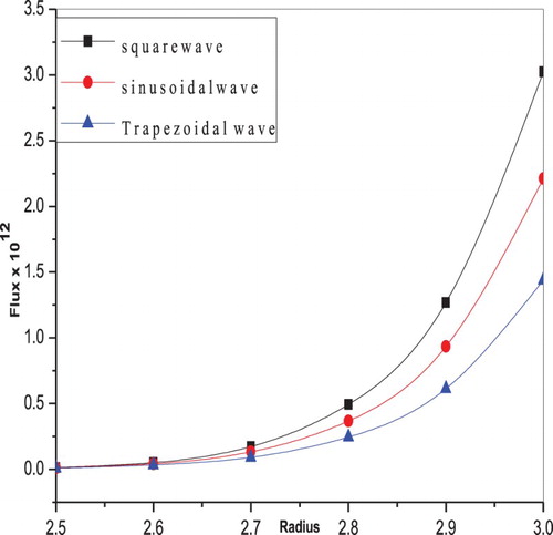The variation of flux as a function of tube radius for different peristaltic wave forms is calculated using Equation (44) and presented in Figure 7. It is clear that the flux is more in the case of square wave when compared to sinusoidal and trapezoidal wave forms.

Figure 2. Variation of flux $F$ with radius for different values of the power-law index $n$ when $t_1=13,t_2=300,\phi =0.6,z=0.1,{{\alpha }_1}^{\mathrm{\prime \prime }}=0.2,{{\alpha }_2}^{\mathrm{\prime \prime }}=0.3$ (for shear thinning fluid).

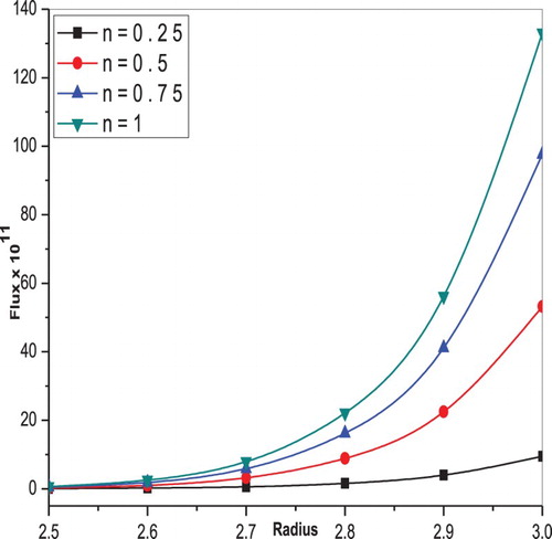
Figure 3. Variation of flux $F$ with radius for different values of amplitude ratio $\phi$ when $t_1=13,t_2=300,n=0.333,z=0.1,{{\alpha }_1}^{\mathrm{\prime \prime }}=0.2,{{\alpha }_2}^{\mathrm{\prime \prime }}=0.3$.

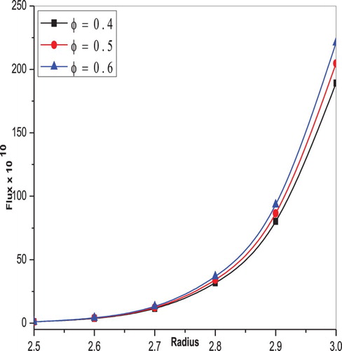
Figure 4. Variation of flux $F$ with outlet pressure for different values of inlet pressure $p_i-p_e$ $t_1=13,t_2=300,\phi =0.6,z=0.1,n=0.333$.

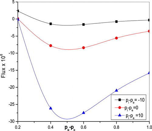
Figure 5. Variation of flux $F$ with inlet pressure for different values of outlet pressure $p_o-p_e$ $t_1=13,t_2=300,\phi =0.6,z=0.1,n=0.333$.

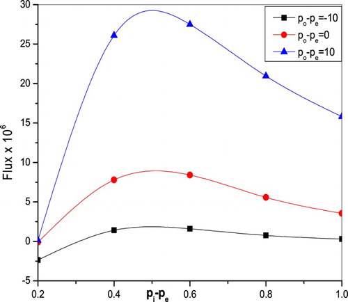
Figure 6. Variation of flux $F$ with radius for different values of the power-law index when $n$ $t_1=13,t_2=300,\phi =0.6,z=0.1,{{\alpha }_1}^{\mathrm{\prime \prime }}=0.2,{{\alpha }_2}^{\mathrm{\prime \prime }}=0.3$ (shear thickening fluids).

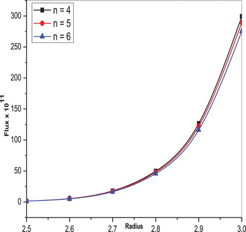
Figure 7. Variation of flux $F$ with radius for different peristaltic wave forms when $t_1=13,t_2=300,n=0.333,z=0.1,{{\alpha }_1}^{\mathrm{\prime \prime }}=0.2,{{\alpha }_2}^{\mathrm{\prime \prime }}=0.3,\phi =0.6$.

The flux variation along the $z$-axis for different values of amplitude ratio $\phi$ and fluid behaviour index $n$ is shown in Figures 8 and 9, respectively. The volume flow rate increases with increasing values of $\phi \text{and}n$. The change in volume flow rate of a power-law fluid in an elastic tube for different values of inlet and outlet radius parameters ${{\alpha }_1}^{\mathrm{\prime \prime }}$ and ${{\alpha }_2}^{\mathrm{\prime \prime }}$ are presented in Figures 10 and 11, respectively. It is clear that the flux decreases for increasing values of the inlet radius parameter, whereas the opposite behaviour is noticed in that the flux increases as outlet radius parameter increases. Also, the flux increases with increasing values of both elastic parameters $t_1\text{and }{t}_2$, which are shown in Figures 12 and 13, respectively. 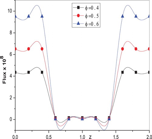The variation of flux along the $z$-axis for trapezoidal wave and square wave forms with different values of amplitude ratio $\phi$ are shown in Figures 14 and 15, respectively. It is found that the flux enhances as amplitude ratio increases in both trapezoidal and square wave cases.

Figure 8. Variation of flux $F$ with $z$-axis for different values of the power-law index when $n$ $t_1=13,t_2=300,\phi =0.6,z=0.1,{{\alpha }_1}^{\mathrm{\prime \prime }}=0.2,{{\alpha }_2}^{\mathrm{\prime \prime }}=0.3$.

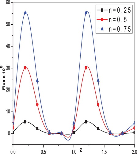
Figure 9. Variation of flux $F$ with $z$-axis for different values of amplitude ratio $\phi$ when $t_1=13,t_2=300,n=0.333,z=0.1,{{\alpha }_1}^{\mathrm{\prime \prime }}=0.2,{{\alpha }_2}^{\mathrm{\prime \prime }}=0.3$.

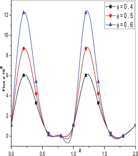
Figure 10. Variation of flux $F$ with $z$-axis for different values of inlet radius parameter when ${\alpha }_1^{\mathrm{\prime \prime }}$ $t_1=13,t_2=300,n=0.333,z=0.1,{{\alpha }_2}^{\mathrm{\prime \prime }}=0.3,\phi =0.5$.

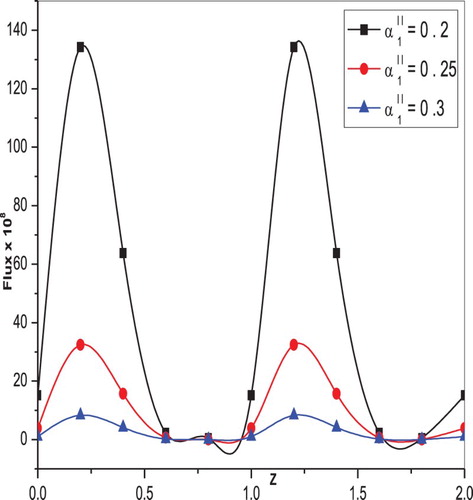
Figure 11. Variation of flux $F$ with $z$-axis for different values of outlet radius parameter when ${\alpha }_2^{\mathrm{\prime \prime }}$ $t_1=13,t_2=300,n=0.333,z=0.1,{{\alpha }_1}^{\mathrm{\prime \prime }}=0.3,\phi =0.5$.

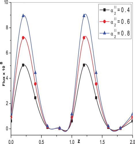
Figure 12. Variation of flux $F$ with $z$-axis For different values of the elastic parameter when $t_1$ $t_2=300,n=0.333,z=0.1,{{\alpha }_1}^{\mathrm{\prime \prime }}=0.2,{{\alpha }_2}^{\mathrm{\prime \prime }}=0.3,\phi =0.5$.

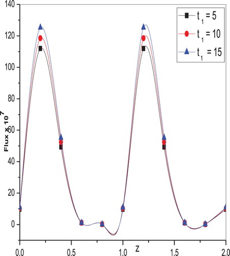
Figure 13. Variation of flux $F$ with $z$-axis for different values of the elastic parameter when $t_2{t}_1=13,n=0.333,z=0.1,{{\alpha }_1}^{\mathrm{\prime \prime }}=0.2,{{\alpha }_2}^{\mathrm{\prime \prime }}=0.3,\phi =0.5$.

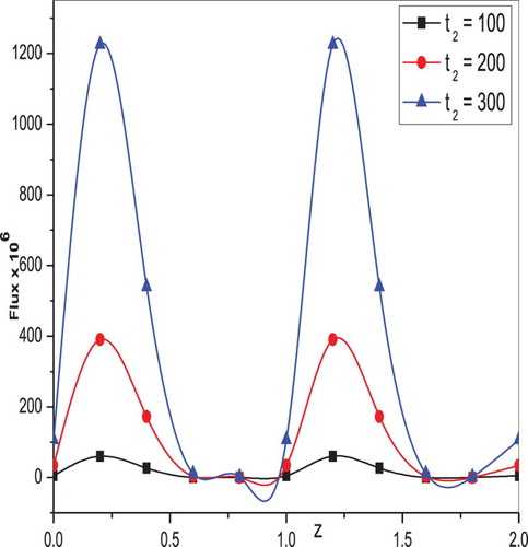
Figure 14. Variation of flux $F$ with $z$-axis for different values of amplitude ratio when $\phi$ $t_1=13,t_2=300,n=0.333,z=0.1,{{\alpha }_1}^{\mathrm{\prime \prime }}=0.2,{{\alpha }_2}^{\mathrm{\prime \prime }}=0.3$ (for Trapezoidal wave).

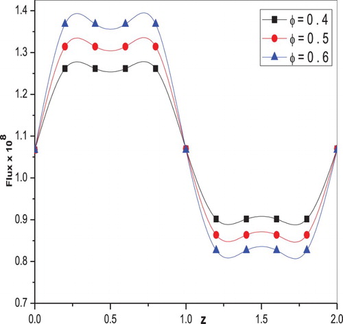
Figure 15. Variation of flux $F$ with $z$-axis for different values of amplitude ratio when $\phi$ $t_1=13,t_2=300,n=0.333,z=0.1,{{\alpha }_1}^{\mathrm{\prime \prime }}=0.2,{{\alpha }_2}^{\mathrm{\prime \prime }}=0.3$ (for Square wave).

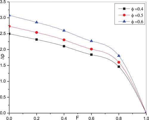
The influence of power-law index $n$, radius ${\alpha }^{\mathrm{\prime \prime }}$ and amplitude ratio $\phi$ on pressure rise $\mathrm{\Delta }p$ along flow rate is represented in the Figure 16–18, respectively. It is observed that the pressure rise is a deceasing function of flow rate. Figure 16 illustrates that for a given flux, the pressure rise increases as the fluid behaviour index increases. The opposite behaviour is noticed in the case of the radius parameter. That is for a given flux, the pressure rise reduces as ${\alpha }^{\mathrm{\prime \prime }}$ increases, which is shown in Figure 17. The significant effect of amplitude ratio on pressure rise is depicted in Figure 18. It is clear that the pressure rise for a given flux increases as $\phi$ increases.

Figure 16. Pressure rise vs. flux $F$ for different values of the power-law index $n$ with ${\alpha }^{\mathrm{\prime \prime }}=0.3,\phi =0.6$ ${\alpha }^{\mathrm{\prime }}=1+\phi \sin 2\pi z$.

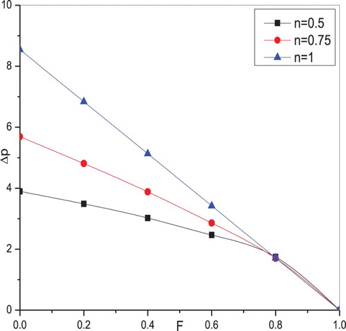
Figure 17. Pressure rise vs. flux $F$ for different values of the radius ${\alpha }^{\mathrm{\prime \prime }}$ with $n=0.333,\phi =0.6$ ${\alpha }^{\mathrm{\prime }}=1+\phi \sin 2\pi z$.

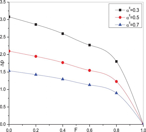
Figure 18. Pressure rise vs. flux $F$ for different values of amplitude ratio $\phi$ with ${\alpha }^{\mathrm{\prime \prime }}=0.3,n=0.3333$ ${\alpha }^{\mathrm{\prime }}=1+\phi \sin 2\pi z$.

The effects of different pertinent parameters on the size of the trapped bolus are presented from Figures 19 to 22. It is found from Figure 19 that the size of the trapped bolus increases as amplitude ratio increases. Another significant observation is that the size of the trapped bolus increases as fluid behaviour index increases, as shown in Figure 20. The effects of inlet and outlet radius parameters on the size of the trapped bolus are studied from Figures 21 and 22, respectively. It is found that the bolus size decreases with increasing values of the inlet radius parameter, whereas the opposite behaviour is observed for the case of outlet radius parameter. The bolus size increases due to an increase in outlet radius parameter.

Figure 19. Streamlines with $n=0.333,{{\alpha }_1}^{\mathrm{\prime \prime }}=0.2,{{\alpha }_2}^{\mathrm{\prime \prime }}=0.3,t_1=13,t_2=300$ and $\left(i\right)\phi =0.4\left(ii\right)\phi =0.5\left(iii\right)\phi =0.6$

Figure 20. Streamlines with $\phi =0.3,{{\alpha }_1}^{\mathrm{\prime \prime }}=0.2,{{\alpha }_2}^{\mathrm{\prime \prime }}=0.3,t_1=13,t_2=300$ and $\left(i\right)n=0.1\left(ii\right)n=0.2\left(iii\right)n=0.3$.

Figure 21. Streamlines with $n=0.393,t_1=13,t_{2}300,\phi =0.4,{{\alpha }_2}^{\mathrm{\prime \prime }}=0.2$ and $\left(i\right){{\alpha }_1}^{\mathrm{\prime \prime }}=0.3\left(ii\right){{\alpha }_1}^{\mathrm{\prime \prime }}=0.4\left(iii\right){{\alpha }_1}^{\mathrm{\prime \prime }}=0.5$.

Figure 22. Streamlines with $n=0.333,t_1=13,t_{2}300,\phi =0.4,{{\alpha }_1}^{\mathrm{\prime \prime }}=0.2$ and $\left(i\right){{\alpha }_2}^{\mathrm{\prime \prime }}=0.3\left(ii\right){{\alpha }_2}^{\mathrm{\prime \prime }}=0.4\left(iii\right){{\alpha }_2}^{\mathrm{\prime \prime }}=0.5$.

Table 2 shows the comparison between the flux for different values of $t_1$ and $t_2$ with ${\alpha }^{\mathrm{\prime }}=1+\phi \sin 2\pi z,\phi =0.6,z=0.1$. If $t_2=300$ and $t_1=13$. It is observed that the values of flux for present study with $n=1$ are similar to the values of flux for Vajravelu et al. [20], with $n=1,{\tau }_0=0.$ A similar observation is noticed for the case of $t_2=200$ and $t_1=13$.

Table 2. Values of flux for different values of $t_1$ and $t_2$ with ${\alpha }^{\mathrm{\prime }}=1+\phi \sin 2\pi z,\phi =0.6,z=0.1$.

	Flux $Q\times {10}^{11}$ (for $t_2=300,t_1=13$)		Flux $Q\times {10}^{11}$ (for $t_2=200,t_1=13$)
$r$	Present study for $(n=1)$	Vajravelu et al. [20] for $(n=1,{\tau }_0=0)$	Present study for $(n=1)$	Vajravelu et al. [20] for $(n=1,{\tau }_0=0)$
2.5	0.65855	0.65855	0.19713	0.19713
2.6	2.51998	2.51998	0.75183	0.75183
2.7	7.95610	7.95610	2.36906	2.36906
2.8	22.1323	22.1323	6.58194	6.58194
2.9	56.1962	56.1962	16.6978	16.6978
3	133.032	133.032	39.5039	39.5039

9. Conclusions

The present study deals with the peristaltic transport of a generalized Newtonian fluid in an elastic tube under the long wavelength and low Reynolds number approximations. The power-law fluid is considered as a non-Newtonian fluid due to its shear thinning and shear thickening behaviours. The analytic expressions for axial velocity, volume flow rate and stream function are presented. The effects of various physical parameters on volume flow rate are calculated by the Rubinow and Keller method [31]. The trapping phenomenon is explained graphically. The important observations are summarized as follows.

1. The flux as a function of tube radius increases for increasing values of amplitude ratio $\phi$ and fluid behaviour index $n$ (for both shear thinning $(n<1)$ and shear thickening $(n>1)$).

2. The flux as a function of inlet pressure increases as outlet pressure increases, but the opposite behaviour is observed for the case of increasing values of inlet pressure.

3. The flux variation is high in the case of square wave form of peristaltic wave when compared to the sinusoidal and trapezoidal wave forms.

4. The flux along the $z$-axis for different values of $\phi ,n,{{\alpha }_1}^{\mathrm{\prime \prime }},{{\alpha }_2}^{\mathrm{\prime \prime }},t_1$ and $t_2$ are analysed. The flux of a power-law fluid in elastic tube with peristalsis increases for increasing $\phi ,n,{{\alpha }_1}^{\mathrm{\prime \prime }},t_1\text{and }{t}_2$ and decreases as ${{\alpha }_2}^{\mathrm{\prime \prime }}$ increases.

5. The pressure rise increases for a given flux with increasing values of $n\text{and}\phi ,$ where it reduces as ${\alpha }^{\mathrm{\prime \prime }}$ increases.

6. The size of the trapped bolus increases for increasing values of $\phi ,n\text{and }{{\alpha }_2}^{\mathrm{\prime \prime }}$ and it decreases as ${{\alpha }_1}^{\mathrm{\prime \prime }}$ increases.

Disclosure statement

No potential conflict of interest was reported by the authors.

ORCID

C. K. Selvi http://orcid.org/0000-0001-9640-4963

A. N. S. Srinivas http://orcid.org/0000-0003-2533-4034

S. Sreenadh http://orcid.org/0000-0003-1429-1921

References

- Shapiro AH, Jaffrin MY, Weinberg SL. Peristaltic pumping with long wavelengths at low Reynolds number. J Fluid Mech. 1969;37:799–825. doi: 10.1017/S0022112069000899
- Radhakrishnamacharya G. Long wavelength approximation to peristaltic motion of a power law fluid. Rehol Acta. 1982;21:30–35. doi: 10.1007/BF01520703
- Shukla JB, Gupta SP. Peristaltic transport of a power-law fluid with variable consistency. J Biomech Eng. 1982;104:182–186. doi: 10.1115/1.3138346
- Srivastava LM, Srivastava VP. Peristaltic transport of a power-law fluid: application to the ductus efferentes of the reproductive tract. Rheol Acta. 1988;27:428–433. doi: 10.1007/BF01332164
- Rao AR, Mishra M. Peristaltic transport of a power-law fluid in a porous tube. J Non-Newtonian Fluid Mech. 2004;121:163–174. doi: 10.1016/j.jnnfm.2004.06.006
- Vajravelu K, Sreenadh S, Viswanatha Reddy G. Helical flow of a power-law fluid in a thin annulus with permeable walls. Int J Non-linear Mech. 2006;41:761–765. doi: 10.1016/j.ijnonlinmec.2006.03.001
- Hayat T, Ali N. On mechanism of peristaltic flows for power-law fluids. Physica A. 2006;371:188–194. doi: 10.1016/j.physa.2006.03.059
- El Hakeem A, El Naby A, El Misery AEM, et al. Hydrodynamic flow of generalized Newtonian fluid through a uniform tube with peristalsis. Appl Math Comp. 2006;173:856–871. doi: 10.1016/j.amc.2005.04.020
- Srinivas S, Kothandapani M. The influence of heat and mass transfer on MHD peristaltic flow through a porous space with compliant walls. Appl Math Comp. 2009;213:197–208. doi: 10.1016/j.amc.2009.02.054
- Roach MR, Burton AC. The reason for the shape of distensibility curves of arteries. Can J Biochem Physiol. 1957;37:557–570. doi: 10.1139/y59-059
- Whirlow DK, Rouleau WT. Periodic flow of a viscous liquid in a thick-walled elastic tube. Bull Math Biophy. 1965;27:355–370. doi: 10.1007/BF02478411
- Wang DM, Tarbell JM. Nonlinear analysis of flow in an elastic tube (artery): steady streaming effects. J Fluid Mech. 1992;239:341–358. doi: 10.1017/S0022112092004439
- Sankar A, Jayaraman G. Non-linear analysis of oscillatory flow in the annulus of an elastic tube: application to catheterized artery. Phys Fluids. 2001;13:2901–2911. doi: 10.1063/1.1389285
- Johnston BM, Johnston PR, Corney S, et al. Non-Newtonian blood flow in human right coronary arteries: steady state simulations. J Bio Mech. 2004;37:709–720.
- Sharma GC, Jain M, Kumar A. Performance modeling and analysis of blood flow in elastic arteries. Math Comput Model. 2004;39:1491–1499. doi: 10.1016/j.mcm.2004.07.006
- Pandey SK, Chaube MK. Peristaltic transport of a visco-elastic fluid in a tube of non-uniform cross section. Math Computer Model. 2010;52:501–514. doi: 10.1016/j.mcm.2010.03.047
- Takagi D, Balmforth J. Peristaltic pumping of viscous fluid in an elastic tube. J Fluid Mech. 2011;672:196–218. doi: 10.1017/S0022112010005914
- Vajravelu K, Sreenadh S, Devaki P, et al. Mathematical model for a Herschel-Bulkley fluid flow in an elastic tube. Cent Eur J Phys. 2011;9:1357–1365.
- Sochi T. The flow of Newtonian and power law fluids in elastic tubes. Int J Non Linear Mech. 2014;67:245–250. doi: 10.1016/j.ijnonlinmec.2014.09.013
- Vajravelu K, Sreenadh S, Devaki P, et al. Peristaltic transport of a Herschel-Bulkley fluid in an elastic tube. Heat Transf-Asian Res. 2015;44:585–598. doi: 10.1002/htj.21137
- Chaube MK, Tripathi D, Anwar Beg O, et al. Peristaltic creeping flow of power law physiological fluids through a non-uniform channel with slip effect. Appl Bionics Biomech. 2015. doi: 10.1155/2015/152802
- Ali N, Javid K, Sajid M, et al. Numerical simulation of peristaltic flow of a biorheological fluid with shear-dependent viscosity in a curved channel. Comput Methods Biomech Biomed Engin. 2016;19:614–627. doi: 10.1080/10255842.2015.1055257
- Vajravelu K, Sreenadh S, Devaki P, et al. Peristaltic pumping of a Casson fluid in an elastic tube. J Appl Fluid Mech. 2016;9:1897–1905. doi: 10.18869/acadpub.jafm.68.235.24695
- Prakash J, Ramesh K, Tripathi D, et al. Numerical simulation of heat transfer in blood flow altered by electroosmosis through tapered micro-vessels. Microvasc Res.. 2018;118:162–172. doi: 10.1016/j.mvr.2018.03.009
- Chaube MK, Yadav A, Tripathi D, et al. Electroosmotic flow of biorheological micropolar fluids through microfluidic channels. Korea-Australia Rheol J. 2018;30:89–98. doi: 10.1007/s13367-018-0010-1
- Prakash J, Tripathi D. Electroosmotic flow of Williamson ionic nanoliquids in a tapered microfluidic channel in presence of thermal radiation and peristalsis. J Mol Liq. 2018;256:352–371. doi: 10.1016/j.molliq.2018.02.043
- Batti MM, Zeeshan A, Tripathi D, et al. Thermally developed peristaltic propulsion of magnetic solid particles in biorheological fluids. Indian J Phys. 2018;92:423–430. doi: 10.1007/s12648-017-1132-x
- Tripathi D, Jhohar R, Beg OA, et al. Electro osmosis modulated peristaltic biorheological flow through an asymmetric microchannel: mathematical model. Maccanica. 2018;53:20179–22090.
- Tripathi D, Borode A, Jhohar R, et al. Computer modelling of electro-osmotically augmented three-layered microvascular peristaltic blood flow. Microvasc Res.. 2017;114:65–83. doi: 10.1016/j.mvr.2017.06.004
- Bird RB, Stewart WE, Lightfoot EN. Transport phenomenon. New York: Wiley; 1960.
- Rubinow SI, Keller JB. Flow of a viscous fluid through an elastic tube with applications to blood flow. J Theor Biol. 1972;35:299–313. doi: 10.1016/0022-5193(72)90041-0
- Flaherty JE, Keller JB, Rubinow SI. Post buckling behavior of elastic tubes and rings with opposite sides in contact. SIAM J Appl Math. 1972;23:446–455. doi: 10.1137/0123047
- Cheremisinoff NP. Encyclopedia of fluid mechanic. Rheology, and non-Newtonian flows. Houston (TX): Gulf Publishing Co.; 1988.