
 ?Mathematical formulae have been encoded as MathML and are displayed in this HTML version using MathJax in order to improve their display. Uncheck the box to turn MathJax off. This feature requires Javascript. Click on a formula to zoom.
ABSTRACT
The Chebyshev Wavelet Method (CWM) is applied to evaluate the numerical solutions of some systems of linear fractional Voltera integro differential equations (FVIDEs). The applicability and validity of the proposed method is ensured by discussing some illustrative examples. The numerical results obtained by this technique are compared with the exact solutions of the problems. The error analysis reveals that the accuracy of the present method is higher than any existing numerical method.
1. Introduction
The theory and applications of fractional calculus can be observed in many fields of science and engineering such as nonlinear oscillation of earth quakes [Citation1], fluid dynamic traffic [Citation2] and signal processing [Citation3].
Due to precious contribution of fractional calculus in various fields of science and engineering, the researchers have shown great interest to study fractional calculus. In this regard as in many cases, it is very difficult to find the exact or analytical solutions of fractional differential and integral equations. The numerical methods have gained importance to avoid this difficulty. Initially, the authors have used different numerical techniques to find the approximate solution of fractional differential and integral equations such as Adomian Decomposition Method (ADM) [Citation4], Spline Collocation Method (SCM) [Citation5], Fractional Transform Method (FTM) [Citation6], Homotopy Perturbation Method (HPM) [Citation7], Operational Tau Method (OTM) [Citation8], Shifted Chebyshev Polynomial Method (SCPM) [Citation9], Rationalized Haar Functions Method (RHFM) [Citation10] and Reproducing Kernel Hilbert Space (RKHSM) [Citation11,Citation12].
Besides these methods, most of the authors have applied a comparatively new numerical techniques based on wavelets [Citation13–16]. The methods based on Chebyshev wavelets have gained much importance during the last decade because of its simple, effective and straightforward implementation. Therefore, the mathematician paid great attention to these methods for solving problems in different fields of science and engineering. Examples are Chebyshev Wavelet Operational Matrix (CWOM) [Citation17], Chebyshev Finite Difference Method (CFDM) [Citation18], Shifted Chebyshev Polynomial Method (SCPM) [Citation9] and Chebyshev Wavelet Method (CWM) [Citation19,Citation20].
The solution to fractional system of differential equations is also a point of investigation for many researchers. Therefore, they introduced and extended many numerical techniques for solving these fractional systems of differential equations. Examples are Adomian Decomposition Method (ADM) [Citation21] and B-Spline method [Citation22].
In this paper, we approximate the solution of fractional systems of Volterra Integro Differential Equations using an efficient Chebyshev Wavelet method (CWM). The simulations are done by the present method and a very useful Chebyshev Wavelet algorithm is developed. The numerical results found by the present method are compared with exact solution of the problem, showing the greatest degree accuracy.
2. Preliminaries and definitions
In this section, we present some definitions and other mathematical preliminaries for the completion of the current work.
Definition 2.1:
The Riemann fractional integral operator of order
on the usual Lebesgue space
is given by
(1)
(1)
This integral operator has the following properties
,
Definition 2.2:
The Caputo definition of fractional differential operator is given by
where
is an integer
It has the following two basic properties
3. Properties of the Chebyshev wavelets
Wavelets consist of family of functions generated from the dilation and translation
of a single function
called the mother wavelet. When the dilation
and translation
change continuously, then we get the following continuous family of Wavelet [Citation19]
If we restrict the parameters
and
to discrete values as
We have the following family of discrete wavelets
where
form a wavelet basis for
. Especially when
and
, then
forms an orthogonal basis.
The second kind of Chebyshev wavelets is constituted of four parameters, , where
is any positive integer,
is the degree of the second Chebyshev polynomial. The Chebyshev wavelets are defined on the interval
as
where
(2)
(2)
Here, are the second Chebyshev polynomials of degree
with respect to the weight function
on the interval [−Citation1,Citation1], and satisfying the following recursive formula
Lemma 3.1:
If the Chebyshev Wavelet expansion of a continuous function converges uniformly, then the Chebyshev Wavelet expansion converges to the function
.
Proof:
See [Citation23].
Theorem 3.2:
A function , with bounded second derivative, say
, can be expanded as an infinite sum of Chebyshev wavelets, and the series converges uniformly to
, that is,
Proof:
See [Citation23].
4. Chebyshev wavelet method (CWM)
In this paper, we consider the fractional systems of Volterra integro differential equations
where
And
(3)
(3)
with the initial conditions
The solution to system (3) can be expended by Chebyshev wavelets series as
(4)
(4) where
is given by Equation Equation(1)
(1)
(1) . The series in Equation Equation(4)
(5)
(5) are truncated as
(5)
(5)
This implies that there are
conditions to determine
coefficients
,
, … ,
. We put these coefficients in Equation Equation(5)
(6)
(6) to obtain the approximate solution by Chebyshev Wavelet method (CWM).
In this article, we considered fractional volterra systems of order one or less than one, two or less than two and three or less than three.
First, we consider system of order one or less than one, which consists of two equations and two unknowns.
with initial conditions
The procedure is as follows, the initial conditions for both
and
are approximated as
(6)
(6)
(7)
(7)
(8)
(8)
(9)
(9)
The remaining conditions can be obtain by substituting Equation Equation(4)
(5)
(5) in Equation Equation(3)
(3)
(3) , by taking
,
, and
, we get
(10)
(10)
(11)
(11)
Assume that Equations (10) and (11) are exact at points. Then
points are calculated by the following formula
The combination of Equations (6), (7), (8), (9), (10) and (11) forms the linear system of
linear equations. The unknown
and
are calculated through the solution of this system.
The same procedure can be repeated for other initial value fractional systems of Volterra Integro differential equations.
5. Numerical examples
Example 5.1 :
Consider the following fractional system of Volterra Integro differential equation of order,
with initial conditions
The exact solution of the system is
and
Table , analysed the approximate solutions for Example 5.1 for different values of such that
. This investigation shows that as the value of
increases from 0.75 to 1, the accuracy is increasing and attained its maximum accuracy at
.
Table 1. The numerical results of Example 5.1.
Table 2. Numerical results of Example 5.1, for different fractional order .
Figure 1. The solution graph of Example 5.1, for at different fractional order.
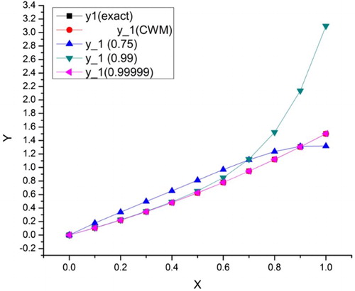
Figure 2. The solution graph of Example 5.1, for at different fractional order.
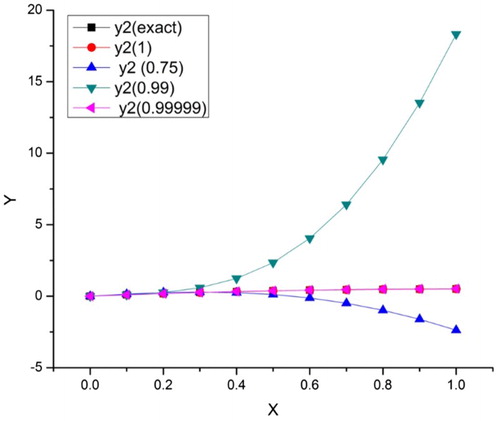
In Table , Error, Error
and Error
show the respective errors of
at
, 0.99 and 0.99999. Similarly, Error
, Error
and Error
are the errors generated with
for
, 0.99 and 0.99999. The error analysis again investigates that solutions at different values of
converges to integer order solutions (Figures and ).
Table 3. Errors of Example 5.1, for different fractional order .
Example 5.2:
Consider the following fractional system of Volterra integro differential equation of order,
With the initial conditions are
The exact solution of the system is ,
,
Table explained the numerical results of Example 5.2. The exact solutions for ,
and
are given by
(exact),
(exact) and
(exact), respectively. The approximate solutions obtained by Chebyshev wavelet method, for
,
and
, are
(CWM),
(CWM) and
(CWM), respectively.
Table 4. The numerical solutions of Example 5.2.
Table analysed the errors associated with the solutions ,
and
for
. These errors are denoted by Error
, Error
and Error
. The absolute error between the exact and approximate solution is obtained which shows the desired degree of accuracy. The numerical simulations are handled by using
and
in the current method.
Table 5. The errors of Example 5.2 for .
In Table , the numerical solutions of Example 5.2 for ,
and
are given at different fractional orders
such that
. Here,
,
and
.
Table 6. Numerical results of Example 5.2 for different orders .
Table emphasizes on error analysis. The errors for all ,
and
are computed at different fractional orders. This error analysis shows the error decreases as the fractional order approaches to integer order (Figures –).
Figure 3. Solution graph of Example 5.2 for at different fractional order.
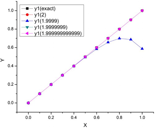
Figure 4. Solution graph of Example 5.2 for at different fractional order.
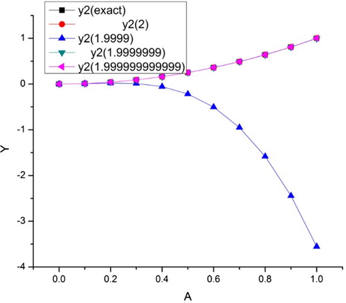
Figure 5. Solution graph of Example 5.2 for at different fractional order.
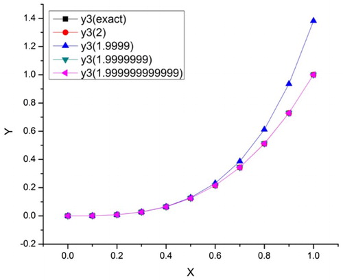
Table 7. The error analysis of Example 5.2 for different order.
Example 5.3:
Consider the following fractional system of Volterra Integro differential equation of order,
with the initial conditions
The exact solution of the system is
Table 8. Numerical results for Example 5.3.
Table expresses the error analysis of Example 5.3 for different fractional orders. The error analysis shows that there is a very small change between the numerical solution at fractional order as compared to integer order (Figures –).
Figure 6. The graph of and
of Example 5.3.
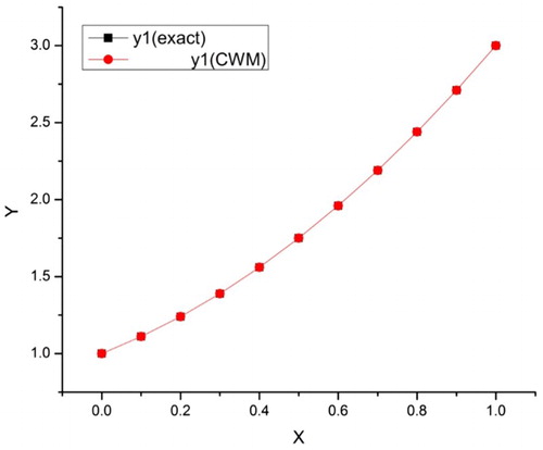
Figure 7. The solution graph of and
.
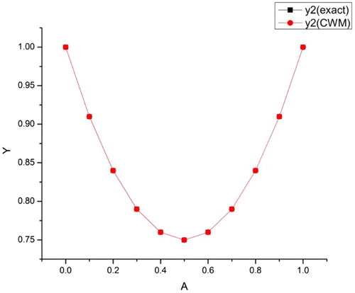
Figure 8. The error graph of and for other fractional orders.
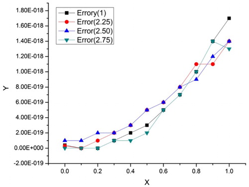
Figure 9. The error graph of for different fractional order
, where
.
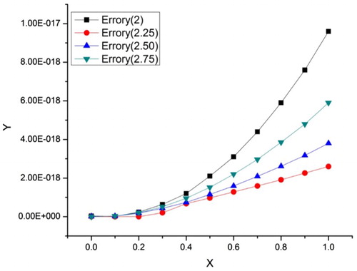
Table 9. The numerical results of Example 5.3, for fractional orders,.
6. Conclusion
In this work, we have fully attempted to find the numerical solution of the fractional system of Volterra Integro differential equations by using Chebyshev wavelet method. The numerical procedure and methodology are done in a very straight forward and effective manner. The numerical accuracy is also a point of interest. During numerical simulations, we observed that the current method has the highest degree of accuracy. On the bases of current work, the researchers can extended this technique to some other fractional systems of ordinary and partial differential equations.
Disclosure statement
No potential conflict of interest was reported by the authors.
ORCID
Hassan Khan http://orcid.org/0000-0001-6417-1181
Muhammad Arif http://orcid.org/0000-0003-1484-7643
References
- He JH. Nonlinear oscillation with fractional derivative and its applications. Int Conf Vibr Eng Dalian (China). 1998;15(2):288–291.
- He JH. Some applications of nonlinear fractional differential equations and their approximations. Bull Sci Technol. 1999;15(2):86–90.
- Panda R, Dash M. Fractional generalized splines and signal processing. Signal Process. 2006;86:2340–2350. doi: 10.1016/j.sigpro.2005.10.017
- El-Sayed WG, El-Sayed AM. On the functional integral equations of mixed type and integro-differential equations of fractional orders. Appl Math Comput. 2004;154:461–467.
- Peedas A, Tamme E. Spline collocation method for integro-differential equations with weakly singular kernels. J Comput Appl Math. 2006;197:253–269. doi: 10.1016/j.cam.2005.07.035
- Nazari D, Shahmorad S. Application of the fractional differential transform method to fractional-order integro-differential equations with nonlocal boundary conditions. J Comput Appl Math. 2010;234:883–891. doi: 10.1016/j.cam.2010.01.053
- Ghazanfari B, Ghazanfari AG, Veisi F. Homotopy perturbation method for nonlinear fractional integro-differential equations. Aust J Basic Appl Sci. 2010;4(12):5823–5829.
- Karimi Vanani S, Aminataei A. Operational Tau approximation for a general class of fractional integro-differential equations. Comput Appl Math. 2011;30(3):655–674. doi: 10.1590/S1807-03022011000300010
- Farhood AK. The solution of nonlinear fractional integro-differential equations by using shifted Chebyshev polynomials method and Adomian decomposition method. Int J Edu Sci Res. 2015;5(3):37–50.
- Ordokhani Y, Rahimi N. Numerical solution of fractional Volterra Integro-differential equations via the rationalized Haar functions. J Sci Kharazmi University. 2014;14(3):211–224.
- Bushnaq S, Momani S, Zhou Y. A reproducing Kernel Hilbert space method for solving integro-differential equations of fractional order. J Optim Theory Appl. 2012;156(1):96–105. doi: 10.1007/s10957-012-0207-2
- Bushnaq S, Maayah B, Momani S, Alsaedi A. A reproducing Kernel Hilbert space method for solving systems of fractional integrodifferential equations. Abstr Appl Anal. 2014 :Article ID 103016, doi.org/10.1155/2014/103016.
- Mohammadi F, Hosseini MM, Mohyud-Din ST. Legendre wavelet Galerkin method for solving ordinary differential equations with nonanalytical solution. Int J Syst Sci. 2011;42(4):579–585. doi: 10.1080/00207721003658194
- Yousefi S, Banifatemi A. Numerical solution of Fredholm integral equations by using CAS wavelets. Appl Math Comp. 2006;183:458–463.
- Cattani C, Kudreyko A. Harmonic wavelet method towards solution of the Fredholm type integral equations of the second kind. Appl Math Comp. 2010;215:4164–4171. doi: 10.1016/j.amc.2009.12.037
- Aziz I, Islam SU, Sarler B. Wavelet collocation methods for the numerical solution of elliptic BV problems. Appl Math Model. 2013;37:676–694. doi: 10.1016/j.apm.2012.02.046
- Babolian E, Fattah Zadeh F. Numerical solution of differential equations by using Chebyshev wavelet operational matrix of integration. Appl Math Comput. 2007;188:417–426.
- Dehghan M, Saadatmandi A. Chebyshev finite difference method for Fredholm integro-differential equation. Int J Comput Math. 2008;85(1):123–130. doi: 10.1080/00207160701405436
- Zhu L, Fa Q. Solving fractional nonlinear Fredholm integro-differential equations by the second kind Chebyshev wavelet. Commun Nonlinear Sci Numer Simulat. 2012;17:2333–2341. doi: 10.1016/j.cnsns.2011.10.014
- Iqbal MA, Ali A, Mohyud-Din ST. Chebyshev wavelets method for fractional boundary value problems. Int J Math Sci. 2014;11(3):152–163.
- Jafari H, Daftardar-Gejji V. Solving a system of nonlinear fractional differential equations using Adomian decomposition. J Comput Appl Math. 2006;196(2):644–651. doi: 10.1016/j.cam.2005.10.017
- Al-Marashi AA. Approximate solution of the system of linear fractional integro-differential equations of Volterra using B-spline method. J Am Res Math Stat. 2015;3(2):39–47.
- Adibi H, Assari P. Chebyshev wavelet method for numerical solution of Fredholm integral equations of the first kind. Math Prob Eng. 2010; Article ID 138408, 17 pages. doi:10.1155/2010/138408.