Laguerre wavelets collocation method for the numerical solution of the Benjamina–Bona–Mohany equations

ABSTRACT

In this paper, a new approach for the accurate numerical solution of the Benjamin–Bona–Mahony (BBM) equations with the initial and boundary conditions using Laguerre wavelets is presented. This method is based on the truncated Laguerre wavelet expansions used to convert the initial and boundary value problems into systems of algebraic equations which can be efficiently solved by suitable solvers. Illustrative examples are included to demonstrate the validity and applicability of the technique. Numerical results show the efficiency and accuracy of the present method.

KEYWORDS:

• Laguerre wavelets
• linear and nonlinear Benjamin–Bona–Mahony (BBM) equations
• collocation method

MSC:

• 35-XX
• 42c40
• 65l60

1. Introduction

Since 1990's [1] wavelet methods have been applied for solving partial differential equations (PDEs). The investigation of the approximate solutions for linear and nonlinear partial differential equations plays an important role in the study of linear and nonlinear physical phenomena. Linear and nonlinear wave phenomena appear in various scientific and engineering fields, such as plasma physics, fluid mechanics, biology, solid state physics, optical fibres, chemical physics, chemical kinematics. Moreover, obtaining the exact solutions for these problems is quite untouched. However, in recent years, numerical analysis [2] has considerably been developed to be used for partial equations such as Benjamina–Bona–Mohany (BBM) equations that have a special kind of solutions. In the present work, Laguerre wavelets have been applied. In most cases the Laguerre wavelets coefficients have been calculated by collocation method, We considerd the nonlinear Benjamina–Bona–Mohany (BBM) equations of the following form: (1) $\begin{array}{rl}& y_t\left(x,t\right)+a{y}_x\left(x,t\right)+by\left(x,t\right)y_x\left(x,t\right)-c{y}_{xxt}\left(x,t\right)\\ & =df\left(x,t\right),\end{array}$(1) where $a$, $b$, $c$ and $d$ are known constants, $f\left(x,t\right)$ is continuous real-valued function on $\left[0,1\right)\times \left[0,1\right)$. Now a days, much attention has been given to the literature of the stable methods for the numerical solution of Benjamina–Bona–Mohany (BBM) equations. In addition to that, Considerable efforts have been made by many mathematicians to obtain exact and approximate solutions of partial differential equations such as Benjamina–Bona–Mohany equations and a number of efficient, accurate and powerful methods have been developed by those mathematicians such as, Backlund transformation method [3], Lie group method [4], Adomian's decomposition method [5], Integral method [6], Hirota's bilinear method [7], homotopy analysis method [8], He's Homotopy perturbation method [9], Exp-Function method [10], Haar wavelet method [11] and Cardinal B-Spline wavelets method [12].

The aim of the present work is to develop Laguerre wavelets collocation method, mutually for solving partial differential equations with initial and boundary conditions of the BBM equations, which is simple, fast and guarantees the necessary accuracy for a relative small number of grid points. A vast amount of literature is available on numerical solution of partial differential equations by Haar wavelet [11], Cardinal B-Spline wavelets [12], Chebyshev wavelet [13], Legendre wavelet [14], Hermite wavelet, etc. but the literatures on Laguerre wavelets to solve PDE's are less this impetused us to obtain numerical solution for PDEs such as BBM equations using Laguerre wavelets.

The outline of this article is as follows: In Section 2 we describe properties of Laguerre wavelets and function approximation. In Section 3 we draw convergence analysis. In Section 4 we describe the Laguerre wavelet method to find the approximate solution of the BBM problems. In Section 5 some numerical examples are solved by applying the Laguerre wavelet method of this article. Finally, a conclusion is drawn in Section 6.

2. Laguerre wavelets and function approximation

Wavelets constitute a family of functions constructed from dialation and translation of a single function called mother wavelet. When the dialation parameter $a$ and translation parameter $b$ varies continuously, we have the following family of continuous wavelets: ${\psi }_a{,}_b\left(x\right)=|a{|}^{-1/2}\psi \left(\frac{x-b}{a}\right),\mathrm{\forall }a,b\in R,a\ne 0.$ If we restrict the parameters $a$ and $b$ to discrete values as $a=a_0^{-k}\text{, }b=n{b}_0{a}_0^{-k}\text{, }{a}_0>1,b_0>0.$ We have the following family of discrete wavelets ${\psi }_k{,}_n\left(x\right)=|a{|}^{1/2}\psi \left(a_0^{k}x-n{b}_0\right),\mathrm{\forall }a,b\in R,a\ne 0,$ where ${\psi }_k{,}_n$ form a wavelet basis for $L^2\left(R\right)$. In particular, when $a_0=2$ and $b_0=1$, then ${\psi }_k{,}_n\left(x\right)$ forms an orthonormal basis. Laguerre wavelets are defined as: (2) ${\psi }_{n,m}\left(x\right)=\left\{\begin{array}{ll}\frac{2^{k/2}}{m!}{L}_m\left(2^{k}x-2n+1\right),& \frac{n-1}{2^{k-1}}\le x<\frac{n}{2^{k-1}}\\ 0,& \text{otherwise}\end{array}\right.$(2) where $m=0,1,\dots ,M-1$ and $n=1,2,\dots ,2^{k-1}$ where $k$ is assumed any positive integer. Here $L_m\left(x\right)$ are Laguerre polynomials of degree m with respect to weight function $W\left(x\right)=1$ on the interval $\left[0,\mathrm{\infty }\right)$ and satisfies the following reccurence formula $L_0\left(x\right)=1$, $L_1\left(x\right)=1-x$, $\begin{array}{rl}{L}_{m+2}\left(x\right)& =\frac{\left(2m+3-x\right)L_{m+1}\left(x\right)-\left(m+1\right)L_m\left(x\right)}{m+2},\\ & \text{where }m=0,1,2,\dots \end{array}$

2.1. Function approximation

Any square integrable function g(x) defined over $\left[0,1\right)$ may be expanded by Laguerre wavelets as: (3) $g\left(x\right)=\sum _{n=1}^{\mathrm{\infty }}\sum _{m=0}^{\mathrm{\infty }}{C}_{n,m}{\psi }_{n,m}\left(x\right),,$(3) where ${\psi }_{n,m}\left(x\right)$ is given in Equation (2), $C_{n,m}=⟨g\left(x\right),{\psi }_{n,m}\left(x\right)⟩$ and $⟨,⟩$ denotes the inner product. We approximate $g\left(x\right)$ by truncating the series represented in Equation (3) as, $g\left(x\right)\approx \sum _{n=1}^{2^{k-1}}\sum _{m=0}^{M-1}{C}_{n,m}{\psi }_{n,m}\left(x\right)=A^T\psi \left(x\right),$ where $A$ and $\psi \left(x\right)$ are $2^{k-1}M\times 1$ a matrix, $\begin{array}{rl}{A}^T& =[C_{1,0},\dots C_{1,M-1},C_{2,0},\dots C_{2,M-1},\dots C_{2^{k-1},0},\\ & \dots C_{2^{k-1},M-1}].\end{array}$ $\begin{array}{rl}\psi \left(x\right)& =\left[{\psi }_{1,0}\right(x),\dots {\psi }_{1,M-1}(x),{\psi }_{2,0}(x),\dots {\psi }_{2,M-1}(x),\\ & \dots {\psi }_{2^{k-1},0}\left(x\right),\dots {\psi }_{2^{k-1},M-1}\left(x\right)].\end{array}$ Similarly, an arbitrary function of two variables $y\left(x,t\right)$ defines over $\left[0,1\right)\times \left[0,1\right)$, may be expanded into Laguerre wavelets basis as: $y\left(x,t\right)\approx {\psi }^T\left(t\right)K\psi \left(x\right),$ where ${\psi }^T\left(t\right)=\left({\psi }_{1,0}\right(t),\dots {\psi }_{1,M-1}(t),{\psi }_{2,0}(t),\dots {\psi }_{2,M-1}(t),\dots {\psi }_{2^{k-1},0}(t),\dots {\psi }_{2^{k-1},M-1}(t\left)\right)$, $\psi \left(x\right)=\left({\psi }_{1,0}\right(x),\dots {\psi }_{1,M-1}(x),{\psi }_{2,0}(x),\dots {\psi }_{2,M-1}(x),\dots {\psi }_{2^{k-1},0}(x),\dots {\psi }_{2^{k-1},M-1}(x){)}^T$ and $K=[a_{j,j}{]}_{N\times N}$, $N=2^{k-1}M$.

3. Convergence analysis

Theorem 1.

If a continuous bounded function $y\left(x,t\right)\in L^2\left(R\times R\right)$ defined on $\left[0,1\right)\times \left[0,1\right)$, then the Laguerre wavelets expansion of $y\left(x,t\right)$ converges uniformly to it.

Proof

: Let $y\left(x,t\right)$ be a continuous function defined on $\left[0,1\right)\times \left[0,1\right)$ and $|y\left(x,t\right)|\le \kappa$, where $\kappa$ is a positive real number. Let $y\left(x,t\right)=\sum _{i=1}^{\mathrm{\infty }}\sum _{j=0}^{\mathrm{\infty }}{C}_{i,j}{\psi }_{i,j}\left(x\right){\psi }_{i,j}\left(t\right).$ $C_{i,j}=⟨y\left(x,t\right),{\psi }_{i,j}\left(x\right){\psi }_{i,j}\left(t\right)⟩$ and $⟨,⟩$ denotes inner product. Then Laguerre wavelet coefficients of continuous functions $y\left(x,t\right)$ are defined as: $C_{i,j}={\int }_0^1,{\int }_0^{1}y\left(x,t\right){\psi }_{i,j}\left(x\right){\psi }_{i,j}\left(t\right)dxdt.$ $\begin{array}{rl}{C}_{i,j}& ={\int }_0^1,{\int }_I^{}y\left(x,t\right)\frac{2^{k/2}}{m!}{L}_m\left(2^{k}x-2n+1\right)\\ & {\psi }_{i,j}\left(t\right)dxdt,\text{where }I=\left[\frac{n-1}{2^{k-1}},\frac{n}{2^{k-1}}\right).\end{array}$ Now change the variable $2^{k}x-2n+1=p,$ we obtain $\begin{array}{rl}{C}_{i,j}& =\frac{2^{k/2}}{m!}{\int }_0^1,\left[{\int }_{-1}^{1}y\left(\frac{p-1+2n}{2^k},t\right)L_m\left(p\right)\frac{dp}{2^k},\right]\\ & {\psi }_{i,j}\left(t\right)dt,\end{array}$ $\begin{array}{rl}{C}_{i,j}& =\frac{2^{-k/2}}{m!}{\int }_0^1,\left[{\int }_{-1}^{1}y\left(\frac{p-1+2n}{2^k},t\right)L_m\left(p\right)dp,\right]\\ & {\psi }_{i,j}\left(t\right)dt,.\end{array}$ Using GMVT for integrals $\begin{array}{rl}{C}_{i,j}& =\frac{2^{-k/2}}{m!}{\int }_0^{1}y\left(\frac{\zeta -1+2n}{2^k},t\right){\psi }_{i,j}\left(t\right)dt\\ & \times \left[{\int }_{-1}^1{\text{L}}_m\left(p\right)dp\right],\text{where }\zeta \in \left(-1,1\right)\end{array}$ Since $L_m\left(x\right)$ is continuous and integrable on $\left(-1,1\right)$. Choose $\underset{-1}{\overset{1}{\int }}{L}_m\left(p\right)dp=A$, $C_{i,j}=A\frac{2^{-k/2}}{m!}{\int }_0^{1}y\left(\frac{\zeta -1+2n}{2^k},t\right){\psi }_{i,j}\left(t\right)dt,$ $\begin{array}{rl}{C}_{i,j}& =A\frac{2^{-k/2}}{m!}{\int }_{\frac{n-1}{2^{k-1}}}^{\frac{n}{2^{k-1}}}y\left(\frac{\zeta -1+2n}{2^k},t\right)\\ & \frac{2^{\frac{k}{2}}}{m!}{L}_m\left(2^{k}t-2n+1\right)dt,\end{array}$ Now change the variable $2^{k}t-2n+1=q,$ we obtain $C_{i,j}=\frac{A}{{(m!)}^2}{\int }_{-1}^{1}y\left(\frac{\zeta -1+2n}{2^k},\frac{q-1+2n}{2^k}\right)L_m\left(q\right)\frac{dq}{2^k},$ $C_{i,j}=\frac{A{2}^{-k}}{{(m!)}^2}{\int }_{-1}^{1}y\left(\frac{\zeta -1+2n}{2^k},\frac{q-1+2n}{2^k}\right)L_m\left(q\right)dq,$ Using GMVT for integrals $\begin{array}{rl}{C}_{i,j}& =\frac{A{2}^{-k}}{{(m!)}^2}y\left(\frac{\zeta -1+2n}{2^k},\frac{\eta -1+2n}{2^k}\right){\int }_{-1}^1{L}_m\left(q\right)dq,\\ & \text{where }\eta \in \left(-1,1\right)\end{array}$ Since $L_m\left(x\right)$ is continuous and integrable on $\left(-1,1\right)$. Choose ${\int }_{-1}^1{L}_m\left(q\right)dq=B$, $\begin{array}{rl}{C}_{i,j}& =\frac{AB{2}^{-k}}{{(m!)}^2}y\left(\frac{\zeta -1+2n}{2^k},\frac{\eta -1+2n}{2^k}\right),\\ & \text{where}\eta ,\zeta \in \left(-1,1\right).\end{array}$ Therefore, $\begin{array}{rl}& \left|C_{i,j}|=|\frac{AB{2}^{-k}}{{(m!)}^2}\right|\left|y\left(\frac{\zeta -1+2n}{2^k},\frac{\eta -1+2n}{2^k}\right)\right|,\\ & \text{where}\eta ,\zeta \in \left(-1,1\right).\end{array}$ Since $y\left(x,t\right)$ is bounded. That is, $|y\left(x,t\right)|\le \kappa$, where $\kappa$ is real constant. $\begin{array}{rl}& \left|C_{i,j}|=|\frac{AB{2}^{-k}}{{(m!)}^2}\right|\kappa =\frac{|A||B|\kappa }{{(m!)}^2{2}^k},\\ & \text{where }k\text{is any positive integer}.\end{array}$

Therefore $\sum _{i=0}^{\mathrm{\infty }}\sum _{j=0}^{\mathrm{\infty }}{c}_{i,j}$ is absolutely convergent. Hence the Laguerre wavelet expansion of $y\left(x,t\right)$ is converged uniformly.

Theorem 2

Laguerre wavelets ${\psi }_{i,j}$ are uniformly continuous on interval I [15].

Theorem 3

If ${\psi }_{i,j}:I\to R$ is Uniformly Continuous on subset $I$ of $R$ and $x_n$ is a Cauchy sequence in $I$ then ${\psi }_{i,j}(x_n$ is Cauchy sequence in $R$. (where ${\psi }_{i,j}$ is Laguerre wavelets) [15].

4. Description of the proposed method

In this section, Laguerre wavelets together with collocation method to solve nonlinear BBM equations is presented. Consider the general BBM equation is of the form (4) $\begin{array}{rl}& \alpha y_t\left(x,t\right)+\beta y_x\left(x,t\right)+\chi y\left(x,t\right)y_x\left(x,t\right)-\delta y_{xxt}\left(x,t\right)\\ & =\mu \left(x,t\right),\end{array}$(4) with initial and boundary conditions, $y\left(x,0\right)=f\left(x\right),0\le x\le 1,$ and $y\left(0,t\right)=g_0\left(t\right),y\left(1,t\right)=g_1\left(t\right),\mathrm{\forall }t\ge 0,$ where $\alpha ,\beta ,\chi \text{and }\delta$ are real constants and $f\left(x\right),g_0\left(t\right),g_1\left(t\right)\text{and }\mu \left(x,t\right)$ are continuous real-valued functions. Let us assume that, (5) $y_{xxt}\left(x,t\right)\approx {\psi }^T\left(t\right)K\psi \left(x\right),$(5) (6) $\begin{array}{rl}{\psi }^T\left(t\right)& =\left({\psi }_{1,0}\right(t),\dots {\psi }_{1,M-1}(t),{\psi }_{2,0}(t),\\ & \dots {\psi }_{2,M-1}\left(t\right),\dots {\psi }_{2^{k-1},0}\left(t\right),\dots {\psi }_{2^{k-1},M-1}\left(t\right)),\end{array}$(6) (7) $\begin{array}{rl}\psi \left(x\right)& =\left({\psi }_{1,0}\right(x),\dots {\psi }_{1,M-1}(x),{\psi }_{2,0}(x),\\ & \dots {\psi }_{2,M-1}\left(x\right),\dots {\psi }_{2^{k-1},0}\left(x\right),\dots {\psi }_{2^{k-1},M-1}\left(x\right){)}^T,\end{array}$(7) (8) $K=[a_{j,j}{]}_{N\times N},N=2^{k-1}M.$(8) $K$ represents $N\times N$ Laguerre wavelets coefficients to be determined. Now integrate Equation (5) with respect to t from 0 to t. (9) $y_{xx}\left(x,t\right)=y_{xx}\left(x,0\right)+{\int }_0^1{\psi }^T\left(t\right)\text{K}\psi \left(x\right)dt.$(9) Now integrate Equation (9) with respect to x from 0 to x. (10) $\begin{array}{rl}{y}_x\left(x,t\right)& =y_x\left(0,t\right)+y_x\left(x,0\right)-y_x\left(0,0\right)\\ & +{\int }_0^x{\int }_0^t{\psi }^T\left(t\right)K\psi \left(x\right)dtdx.\end{array}$(10) Now integrate Equation (10) with respect to x from 0 to x. (11) $\begin{array}{rl}y\left(x,t\right)& =y\left(0,t\right)+x\left(y_x\left(0,t\right)-y_x\left(0,0\right)\right)+y\left(x,0\right)\\ & -y\left(0,0\right)+{\int }_0^x{\int }_0^x{\int }_0^t{\psi }^T\left(t\right)K\psi \left(x\right)dtdxdx.\end{array}$(11) put $x=1$ in Equation (11) and by given conditions, we get (12) $\begin{array}{rl}& y_x\left(0,t\right)-y_x\left(0,0\right)=g_1\left(t\right)-g_0\left(t\right)+f\left(0\right)-f\left(1\right)\\ & -{\int }_0^x{\int }_0^x{\int }_0^t{\psi }^T\left(t\right)K\psi \left(x\right)dt\text{d}xdx{|}_{x=1}.\end{array}$(12) Substitute Equation (12) in Equation (11) and (10), we get (13) $\begin{array}{rl}{y}_x\left(x,t\right)& =y_x\left(x,0\right)+g_1\left(t\right)-g_0\left(t\right)+f\left(0\right)-f\left(1\right)\\ & -\underset{0}{\overset{x}{\int }}\underset{0}{\overset{x}{\int }}\underset{0}{\overset{t}{\int }}{\psi }^T\left(t\right)K\psi \left(x\right)dtdxdx{|}_{x=1}\\ & +\underset{0}{\overset{x}{\int }}\underset{0}{\overset{x}{\int }}\underset{0}{\overset{t}{\int }}{\psi }^T\left(t\right)K\psi \left(x\right)dtdxdx.,\end{array}$(13) and (14) $\begin{array}{rl}& y\left(x,t\right)=y\left(0,t\right)+x\left(g_1\right(t)-g_0(t)+f(0)-f(1)\\ & -{\int }_0^x{\int }_0^x{\int }_0^t{\psi }^T\left(t\right)K\psi \left(x\right)dtdxdx{|}_{x=1}\\ & +y\left(x,0\right)-y\left(0,0\right)+{\int }_0^x{\int }_0^x{\int }_0^t{\psi }^T\left(t\right)K\psi \left(x\right)dtdxdx.\end{array}$(14) Now differentiate Equation (14) with respect to t, we get (15) $\begin{array}{rl}{y}_t\left(x,t\right)& =y_t\left(0,t\right)+x\left(g_1^{\mathrm{\prime }}\right(t)-g_0^{\mathrm{\prime }}(t)\\ & -{\int }_0^x{\int }_0^x{\psi }^T\left(t\right)K\psi \left(x\right)dxdx{|}_{x=1}\\ & +{\int }_0^x{\int }_0^x{\psi }^T\left(t\right)K\psi \left(x\right)dxdx.\end{array}$(15) Substituting Equations (15), (14), (13) and (5) in Equation (4) and collocate the obtained equation using following collocation points $x_i,t_i=\frac{2i-1}{M^2},i=1,2,\dots ,M$. Then solve the obtained system by Newton's iterative method. We obtain the Laguerre wavelets coefficients $a_{j,j}$, where $j=1,2,\dots ,2^{k-1}M$, then substitute these obtained Laguerre wavelets coefficients in Equation (14) will contribute the Laguerre wavelets based numerical solution of Equation (4). The absolute error (AE) will be calculated by, $AE=|y_e\left(x,t\right)-y_{app}\left(x,t\right)|$, where $y_e\left(x,t\right)$ and $y_{app}\left(x,t\right)$ are exact and approximate solutions, respectively.

5. Numrical experiments

Test Problem 1. Consider the linear BBM equation of the form [11] $y_t\left(x,t\right)-2y_{xxt}\left(x,t\right)+y_x\left(x,t\right)=0,$ with initial condition $y\left(x,0\right)=e^{-x}0\le x\le 1,$ and boundary conditions $y\left(0,t\right)=e^{-t},y\left(1,t\right)=e^{-1-t},\mathrm{\forall }t\ge 0.$ The exact solution is $e^{-x-t}$. The space–time graph of the approximate solution for $k=1,M=9$ is shown in Fig. 1. 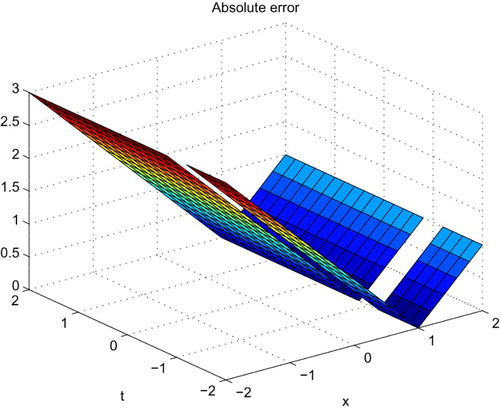The absolute error between the analytical and approximate solutions is shown in the Fig. 2. Fig. 3 represents the comparison of the numerical and exact solution at different values of $t$. 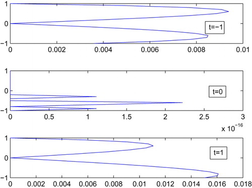The absolute error between the numerical and exact solution is drawn in the Fig. 4 at different values of $t$

Figure 1. Approximate solution of Example 1.

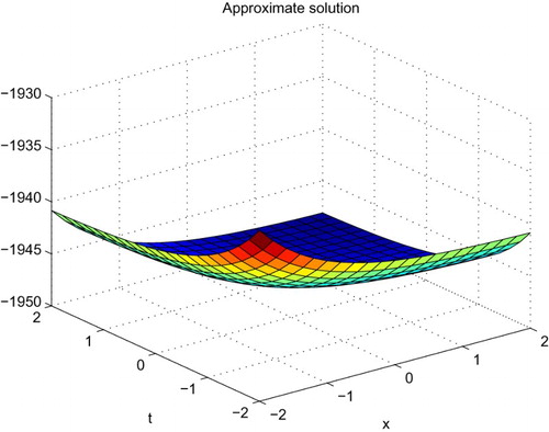
Figure 2. Absolute error of Example 1.

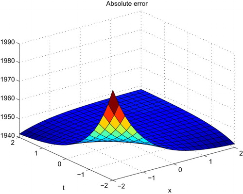
Figure 3. Comparison of numerical and exact solution at different values of $t$ of Example 1.

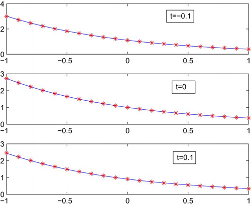
Figure 4. Absolute error in different values of $t$ of example 1.

Test Problem 2. Consider the linear non-homoge-nous BBM equation of the form [11] $y_t\left(x,t\right)-2y_{xxt}\left(x,t\right)+e^{x+t}=0,$ with initial condition $y\left(x,0\right)=e^{x}0\le x\le 1,$ and boundary conditions $y\left(0,t\right)=e^t,y\left(1,t\right)=e^{1+t},\mathrm{\forall }t\ge 0.$ The exact solution is $e^{x+t}$. The space–time graph of the approximate solution for $k=1,M=9$ and the exact solution is shown in Fig. 5. The absolute error between the analytical and approximate solutions is shown in the Fig. 6. Fig. 7 represents the comparison of the numerical and exact solution at different values of $t$. The absolute error between the numerical and exact solution is drawn in the Fig. 8 at different values of $t$

Figure 5. Approximate solution of Example 2.

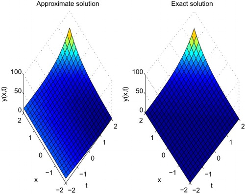
Figure 6. Absolute error of Example 2.

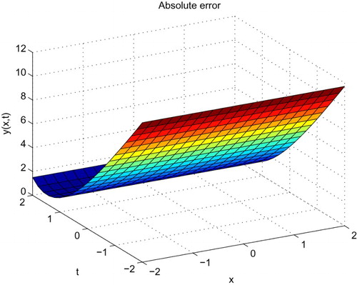
Figure 7. Comparison of numerical and exact solution at different values of $t$ of Example 2.

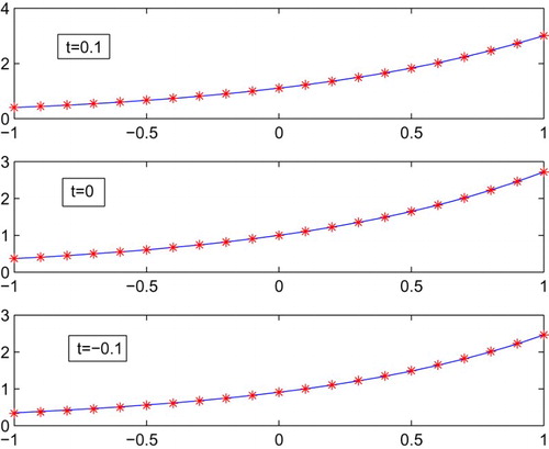
Figure 8. Absolute error in different values of $t$ of example 2.

Test Problem 3. Consider the non-linear BBM equation of the form [11] $y_t\left(x,t\right)-y_{xxt}\left(x,t\right)+y\left(x,t\right)y_x\left(x,t\right)=0,$ with initial condition $y\left(x,0\right)=00\le x\le 1,$ and boundary conditions $y\left(0,t\right)=0,y\left(1,t\right)=\frac{1}{1+t},\mathrm{\forall }t\ge 0.$ The exact solution is $\frac{x}{1+t}$. The space–time graph of the approximate solution for $k=1,M=6$ is shown in Figure 9. The absolute error between the analytical and approximate solutions is shown in Figure 10.

Figure 9. Approximate solution of Example 3.

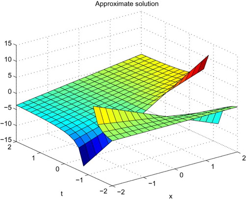
Figure 10. Absolute error of Example 3.

6. Conclusion

In this paper, Laguerre wavelets based collocation method is presented for the solution of linear and nonlinear PDEs such as Benjamina–Bona–Mohany equations for different physical conditions which is important for the development of new research in the field of numerical analysis and beneficial for new researchers. The proposed scheme is tested on some examples and the results are quite satisfactory in comparison with the exact solutions. Finally, we summarize the outcomes of this analysis as follows:

1. The present method gives better accuracy in comparison with the exact solution.

2. This scheme is easy to implement in computer programmes and we can extend this scheme for higher order also with slight modification in the present method.

3. Also, the implementation of the proposed method is very simple and as the obtained numerical results show that, method is very efficient for the numerical solution of the above-mentioned problems and can also be used for numerical solution of other partial differential equations.

4. Properties of Laguerre wavelets and its convergent analysis are discussed in terms of theorems.

Disclosure statement

No potential conflict of interest was reported by the authors.

ORCID

S. Kumbinarasaiah http://orcid.org/0000-0001-8942-7892

Additional information

Funding

It is a pleasure to thank the University Grants Commission (UGC), Govt. of India for the financial support under UGC-SAP DRS-III for 2016-2021:F.510/3/DRS-III/2016(SAP-I) Dated: 29th Feb. 2016.

References

- Lepik U. Solving pdes with the aid of two-dimensional haar wavelets. Comput Math Appl. 2011;61:1873–1879. doi: 10.1016/j.camwa.2011.02.016
- Burden RL, Faires JD. Numerical analysis. Boston, MA: PWS; 1993.
- Rogers C, Shadwich WF. Bäcklund transformations and their application. New York: Academic Press; 1982.
- Olver PJ. Applications of Lie groups to differential equations. Berlin: Springer; 1986.
- Adomian G. A review of the decomposition method in applied mathematics. J Math Anal Appl. 1988;135:501–544. doi: 10.1016/0022-247X(88)90170-9
- Abbasbandy S, Shirzadi A. The first integral method for modified Benjamin–Bona–Mahony equation. Commun Nonlinear Sci Numer Simulat. 2010;15:1759–1764. doi: 10.1016/j.cnsns.2009.08.003
- Hirota R. Exact solution of the Korteweg-de Vries equa-tion for multiple collisions of solitons. Phys Rev Lett. 1971;27:1192–1194. doi: 10.1103/PhysRevLett.27.1192
- Liao SJ. An analytic approach to solve multiple solutions of a strongly nonlinear problem. Appl Math Comput. 2005;169:854–865.
- He JH. Asymptotology by homotopy perturbation method. Appl Math Comput. 2004;156:591–596.
- Ganji ZZ, Ganji DD, Bararnia H. Approximate general and explicit solutions of nonlinear BBMB equations by Exp-function method. Appl Math Model. 2009;33:1836–1841. doi: 10.1016/j.apm.2008.03.005
- Shiralashetti SC, Angadi LM, Deshi AB, et al. Haar wavelet method for the numerical solution of benjamin-bona-mahony equations. J Informat Comput Sci. 2016;11:136–145.
- Shiralashetti SC, Kumbinarasaiah S. Cardinal B-spline wavelet based numerical method for the solution of generalized Burgers–Huxley Equation. Int J Appl Comput Math. 2018. doi: 10.1007/s40819-018-0505-y
- Heydari MH, Hooshmandasl MR, Maalek Ghaini FM. A new approach of the Chebyshev wavelets method for partial differential equations with boundary conditions of the telegraph type. Appl Math Model. 2014;38:1597–1606. doi: 10.1016/j.apm.2013.09.013
- Lahmar NA, Belhamitib O, Bahric SM. A New LegendreWavelets decomposition method for solving PDEs. Malaya J Mat. 2014;1(1):72–81.
- Shiralashetti SC, Kumbinarasaiah S. Theoretical study on continuous polynomial wavelet bases through wavelet series collocation method for nonlinear Lane–Emden type equations. Appl Math Comput. 2017;315:591–602.