
 ?Mathematical formulae have been encoded as MathML and are displayed in this HTML version using MathJax in order to improve their display. Uncheck the box to turn MathJax off. This feature requires Javascript. Click on a formula to zoom.
ABSTRACT
In this paper, we apply the (G′/G)-expansion method based on three auxiliary equations, namely, the generalized Riccati equation , the Jacobi elliptic equation
and the second order linear ordinary differential equation (ODE)
to find many new exact solutions of a nonlinear partial differential equation (PDE) describing the nonlinear low-pass electrical lines. The given nonlinear PDE has been derived and can be reduced to a nonlinear ODE using a simple transformation. Soliton wave solutions, periodic function solutions, rational function solutions and Jacobi elliptic function solutions are obtained. Comparing our new solutions obtained in this paper with the well-known solutions is given. Furthermore, plotting 2D and 3D graphics of the exact solutions is shown.
1. Introduction
In the recent years, investigations of exact solutions to nonlinear PDEs play an important role in the study of nonlinear physical phenomena in such as fluid mechanics, hydrodynamics, optics, plasma physics, solid state physics, biology and so on. Several methods for finding the exact solutions to nonlinear equations in mathematical physics have been presented, such as the inverse scattering method [Citation1], the Hirota bilinear transform method [Citation2], the truncated Painlevé expansion method [Citation3,Citation4], the Bäcklund transform method [Citation5,Citation6], the exp-function method [Citation7–9], the tanh-function method [Citation10–12], the Jacobi elliptic function expansion method [Citation13–15], the (G′/G)-expansion method [Citation16–20], the (G′/G,1/G)-expansion method [Citation21–23], the generalized projective Riccati equations method [Citation24–26] and so on.
The objective of this paper is to use the (G′/G)-expansion method with the aid of Computer algebraic system Maple to construct many exact solutions of the following nonlinear PDE governing wave propagation in nonlinear low-pass electrical transmission lines [Citation15,Citation27]:
(1.1)
(1.1)
where
,
and
are positive real constants, while
is the voltage in the transmission lines. The variable
is interpreted as the propagation distance and
is the slow time. The physical details of the derivation of Equation (1.1) using the Kirchhoff's laws given in [Citation27]. Equation (1.1) has been discussed in [Citation15,Citation27] using a new Jacobi elliptic function expansion method and an auxiliary equation method respectively, and its exact solutions have been found.
This paper is organized as follows: In Section 2, the description of the (G'/G)-expansion method is given. In Section 3, we use the given method described in Section 2, to find exact solutions of Equation (1.1). In Section 4, physical explanations of some results are presented. In Section 5, some conclusions are obtained.
2. Description of the (G'/G)-expansion method
Consider a nonlinear PDE in the form:
where
is a unknown function,
is a polynomial in
and its partial derivatives in which the highest-order derivatives and nonlinear terms are involved. Let us now give the main steps of the (G'/G)-expansion method [Citation16–20]:
Step 1. We look for the voltage in the travelling form:
where
is a positive parameter, and
is the velocity of propagation. To reduce Equation (2.1) to the following nonlinear ODE:
where
is a polynomial of
and its total derivatives
and
.
Step 2. We assume that the solution of Equation (2.3) has the form:
where
are constants to be determined later, provided
and
satisfies the following three auxiliary equations:
(1) The generalized Riccati equation
(2) The Jacobi elliptic equation
(3) The second order linear ODE
Step 3. We determine the positive integer in (2.4) by balancing the highest-order derivatives and the highest nonlinear terms in Equation (2.3).
Step 4. Substituting (2.4) along with Equations (2.5)–(2.7) into Equation (2.3) and collecting all the coefficients of for Equation (2.5),
for Equations (2.6) and (2.7), then setting these coefficients to zero, yield a set of algebraic equations, which can be solved by using the Maple or Mathematica to find the values of
,
and
.
Step 5. It is well-known that Equations (2.5)–(2.7) have many families of solutions obtained in [Citation16–20].
Step 6. Substituting the values of ,
and
as well as the solutions of Step 5, into (2.4) we have the exact solutions of Equation (2.1).
3. On solving Equation (1.1) using the proposed method of Section 2
In this section, we apply the -expansion method of Section 2 to find new exact solutions of Equation (1.1). To this aim, we use the transformation (2.2) to reduce Equation (1.1) to the following nonlinear ODE:
Integrating Equation (3.1) with respect to
twice, and vanishing the constants of integration, we find the following ODE:
where
and
.
Balancing with
gives
. Therefore, (2.4) reduces to
where
and
are constants to be determined such that
.
3.1. Exact solutions of eq. (1.1) depending on the Riccati equation
In this subsection, substituting (3.3) along with the generalized Riccati equation (2.5) into Equation (3.2) and collecting all the coefficients of and setting them to zero, we get a system of algebraic equations for
,
and
. Using the Maple or Mathematica, we get the following results:
Result 1.
Substituting (3.1.1) into (3.3) yields
where
,
,
and
With reference to solving Equation (2.7) [Citation19], we deduce that the exact solutions of Equation (1.1) as follows:
Result 2.
Substituting (3.1.5) into (3.3) yields
where
and
.
In this result, we deduce that the exact solutions of Equation (1.1) as follows:
where
.
where
.
Also, there are many other exact solutions of Equation (1.1), which are omitted here for simplicity.
3.2. Exact solutions of Equation (1.1) depending on the Jacobi elliptic equation
In this subsection, substituting (3.3) along with the Jacobi elliptic equation (2.6) into Equation (3.2) and collecting all the coefficients of and setting them to be zero, we have the following algebraic equations:
On solving the above algebraic equations (3.2.1) using the Maple or Mathematica, we have the following result:
where
Substituting (3.2.2) into (3.3) yields
where
With reference to solving Equation (2.6) [Citation20], we deduce that the Jacobi elliptic functions solutions and other exact solutions of Equation (1.1) as follows:
Case 1. Choosing and
, we obtain the Jacobi elliptic function solutions
where
If , then Equation (1.1) has the kink soliton wave solutions
where
Case 2. Choosing and
, we obtain the Jacobi elliptic function solutions
where
.
If , then we have the same exact solutions (Equation (3.2.5)).
Case 3. Choosing and
, we obtain the Jacobi elliptic function solutions
where
If , then Equation (1.1) has the trigonometric solutions
where
If , then Equation (1.1) has the anti-kink soliton wave solutions
where
Case 4. Choosing and
, we obtain the Jacobi elliptic function solutions
where
.
If , then Equation (1.1) has the trigonometric solutions
where
Case 5. Choosing and
, we obtain the Jacobi elliptic function solutions
where
If , then we have the same exact solutions (Equation (3.2.5)).
Case 6. Choosing and
, we obtain the Jacobi elliptic function solutions
where
If , then we have the same exact solutions (Equation (3.2.8)).
If , then we have the same exact solutions (Equation (3.2.9)).
Case 7. Choosing and
, we obtain the Jacobi elliptic function solutions
where
If , then we have the same exact solutions (Equation (3.2.9)).
Case 8. Choosing and
, we obtain the Jacobi elliptic function solutions
where
If , then we have the same exact solutions (Equation (3.2.5)).
Case 9. Choosing and
, we obtain the Jacobi elliptic function solutions
where
If , then we have the trivial solution.
Case 10. Choosing and
, we obtain the Jacobi elliptic function solutions
where
If , then we have the same exact solutions (Equation (3.2.11)).
3.3. Exact solutions of Equation (1.1) depending on the second order linear ODE
Here, substituting (3.3) along with the second order linear ODE (2.7) into Equation (3.2) and collecting all the coefficients of and setting them to be zero, we have the following algebraic equations:
On solving the above algebraic equations (3.3.1) using the Maple or Mathematica, we have the following result:
Substituting (3.3.2) into (3.3) yields
With reference to solving Equation (2.7) [Citation16–18], we deduce that the hyperbolic functions solutions and the trigonometric functions solutions as follows:
Case 1. If , then we have the hyperbolic functions solutions
In particular, if we set
and
, in (3.3.4), then we get the kink soliton wave solutions
while, if we set and
, then we get the anti-kink soliton wave solutions
where
Case 2. If , then we have the trigonometric functions solutions
In particular, if we set
and
, in (3.3.7), then we get the same kink soliton wave solutions (3.3.5), while, if we set
and
, then we get the same anti-kink soliton wave solutions.
4. Physical explanations of some results
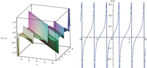
In this section, we have presented some graphs of the exact solutions. These solutions are soliton solutions, periodic solutions and Jacobi elliptic functions solutions. Exact solutions of the results describe different nonlinear waves. For the established exact solutions with hyperbolic solutions are special kinds of solitary waves solutions. Now, let us examine Figures – as it illustrates some of our solutions obtained in this paper. To this aim, we select some special values of the parameters obtained, for example, in some of the solutions (3.1.3), (3.1.7) and (3.2.4) of the nonlinear PDE (1.1). For more convenience, the graphical representations of these solutions are shown in the figures.
Figure 1. The plot of solution (3.1.3) when
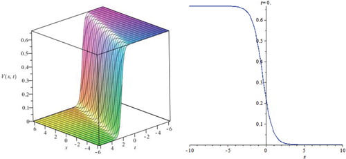
Figure 2. The plot of solution (3.1.7) when
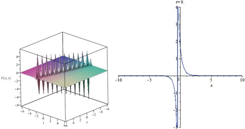
Figure 3. The plot of solution (3.2.4) when
5. Conclusions
In this paper, we have solved the nonlinear PDE describing the nonlinear low-pass electrical transmission lines (1.1) using the (G′/G)-expansion method with the aid of three auxiliary equations (2.5)–(2.6) described in Section 2. By the aid of Maple or Mathematica, we have found many solutions of Equation (1.1) which are new. On comparing our results with the results obtain in [Citation15,Citation27] using the new Jacobi elliptic function expansion method and the auxiliary equation method respectively, we deduce that our results are different and new. Also, we have noted that our results (3.3.5) and (3.3.6) are in agreement with the results (3.2.5) and (3.2.9) of Section 3.2 obtained in this paper respectively, when . Furthermore, all solutions obtained in this paper have been checked with the Maple by putting them back into the original equations. Finally, the proposed method in this paper can be applied to many other nonlinear PDEs in mathematical physics.
Disclosure statement
No potential conflict of interest was reported by the authors.
ORCID
Ayad M. Shahoot http://orcid.org/0000-0003-3483-4110
Khaled A. E. Alurrfi http://orcid.org/0000-0002-0281-0301
Mohamed O. M. Elmrid http://orcid.org/0000-0002-5511-8925
Ali M. Almsiri http://orcid.org/0000-0002-0718-1620
Abdullah M. H. Arwiniya http://orcid.org/0000-0002-5563-6773
References
- Ablowitz MJ, Clarkson PA. Solitons, nonlinear evolution equations and inverse scattering transform. New York (NY, USA): Cambridge University Press; 1991.
- Hirota R. Exact solutions of the KdV equation for multiple collisions of solutions. Phys Rev Lett. 1971;27:1192–1194. doi: 10.1103/PhysRevLett.27.1192
- Weiss J, Tabor M, Carnevale G. The Painlevé property for partial differential equations. J. Math. Phys. 1983;24:522–526. doi: 10.1063/1.525721
- Kudryashov NA. On types of nonlinear nonintegrable equations with exact solutions. Phys Lett A. 1991;155:269–275. doi: 10.1016/0375-9601(91)90481-M
- Rogers C, Shadwick WF. Bäcklund transformations and their applications. New York (NY): Academic Press; 1982.
- Zayed EM, Alurrfi KA. The Bäcklund transformation of the Riccati equation and its applications to the generalized KdV-mKdV equation with any-order nonlinear terms. PanAmerican Math. J. 2016;26:50–62.
- EL-Wakil SA, Madkour MA, Abdou MA. Application of exp-function method for nonlinear evolution equations with variable coefficients. Phys Lett A. 2007;369:62–69. doi: 10.1016/j.physleta.2007.04.075
- Wang YP. Solving the (3+1)-dimensional potential-YTSF equation with Exp-function method 2007 ISDN. J. Phys. Conf. Ser. 2008;96:012186. doi: 10.1088/1742-6596/96/1/012186
- Khan K, Akbar MA. Traveling wave solutions of the (2+1)-dimensional Zoomeron equation and the Burgers equations via the MSE method and the Exp-function method. Ain Shams Eng. J. 2014;5:247–256. doi: 10.1016/j.asej.2013.07.007
- Fan EG. Extended tanh-function method and its applications to nonlinear equations. Phys Lett A. 2000;277:212–218. doi: 10.1016/S0375-9601(00)00725-8
- Zhang S, Xia TC. A further improved tanh-function method exactly solving the (2+1)-dimensional dispersive long wave equations. Appl. Math. E-Notes. 2008;8:58–66.
- Zayed EM, Alurrfi KA. On solving the nonlinear Biswas-Milovic equation with dual-power law nonlinearity using the extended tanh-function method. J Adv. Phys. 2015;11:3001–3012.
- Zheng B, Feng Q. The Jacobi elliptic equation method for solving fractional partial differential equations. Abs. Appl. Anal. 2014; Article ID 249071:9 pages.
- Hong-cai MA, Zhang ZP, Deng A. A new periodic solution to Jacobi elliptic functions of MKdV equation and BBM equation. Acta Math. Appl. Sinica. English series, 2012;28:409–415. doi: 10.1007/s10255-012-0153-7
- Zayed EM, Alurrfi KA. A new Jacobi elliptic function expansion method for solving a nonlinear PDE describing the nonlinear low-pass electrical lines. Chaos Solitons Fractals. 2015;78:148–155. doi: 10.1016/j.chaos.2015.07.018
- Wang M, Li X, Zhang J. The (G'/G)-expansion method and travelling wave solutions of nonlinear evolution equations in mathematical physics. Phys Lett A. 2008;372:417–423. doi: 10.1016/j.physleta.2007.07.051
- Li ZL. Constructing of new exact solutions to the GKdV-mKdV equation with any-order nonlinear terms by (G'/G)-expansion method. Appl. Math. Comput. 2010;217:1398–1403.
- Zayed EM. The (G'/G)-expansion method and its applications to some nonlinear evolution equations in the mathematical physics. J. Appl. Math. Comput. 2009;30:89–103. doi: 10.1007/s12190-008-0159-8
- Zayed EM. The (G'/G)-expansion method combined with the Riccati equation for finding exact solutions of nonlinear PDEs. J. Appl. Math. Inform. 2011;29:351–367.
- Zayed EM, Alurrfi KA. Extended generalized (G'/G)-expansion method for solving the nonlinear quantum Zakharov Kuznetsov equation. Ricerche Mat. 2016;65:235–254. doi: 10.1007/s11587-016-0276-x
- Li Lx, Li QE, Wang M. The (G/G',1/G)-expansion method and its application to traveling wave solutions of the Zakharov equations. Appl. Math. J. Chin. Uni. 2010;25:454–462. doi: 10.1007/s11766-010-2128-x
- Zayed EM, Alurrfi KA. On solving two higher-order nonlinear PDEs describing the propagation of optical pulses in optic fibers using the (G/G',1/G)-expansion method. Ricerche Mat. 2015;64:164–194. doi: 10.1007/s11587-015-0226-z
- Zayed EM, Shahoot AM, Alurrfi KA. The (G/G',1/G)-expansion method and its applications for constructing many new exact solutions of the higher-order nonlinear Schrödinger equation and the quantum Zakharov–Kuznetsov equation. Opt. Quant. Electron. 2018;50. doi: 10.1007/s11082-018-1337-z
- Yan ZY. Generalized method and its application in the higher-order nonlinear Schrodinger equation in nonlinear optical fibres. Chaos Solitons Fractals. 2003;16:759–766. doi: 10.1016/S0960-0779(02)00435-6
- Zayed EM, Alurrfi KA. The generalized projective Riccati equations method and its applications for solving two nonlinear PDEs describing microtubules. Int. J. Phys. Sci. 2015;10:391–402. doi: 10.5897/IJPS2015.4289
- Shahoot AM, Alurrfi KA, Hassan IM, et al. Solitons and other exact solutions for two nonlinear PDEs in mathematical physics using the generalized projective Riccati equations method. Adv. Math. Phys. 2018; (In press).
- Abdoulkary S, Beda T, Dafounamssou O, et al. Dynamics of solitary pulses in the nonlinear low-pass electrical transmission lines through the auxiliary equation method. J. Mod. Phys. Appl. 2013;2:69–87.