Cooperative search model for finding a brownian target on the real line

ABSTRACT

In this paper, we study the cooperation between two searchers start the searching process from the origin to meet a Brownian moving target on a real line. We find the conditions that make the expected value of the first meeting time between one of the searchers and the target is finite. This is the first model which calculates the approximate value for the expected value of the first meeting time. An illustrative example has been given to demonstrate the applicability of this model.

KEYWORDS:

• Linear search
• Coordinated search
• Brownian motion

1. Introduction

In physics, the Brownian motion is useful for studying a variety of natural phenomena such as heat conduction and gases diffusion. Modelling the Brownian particle's movement in the cylinder is one of an interesting physics problems. The aim of this model is to obtain the expected value of the first meeting time between two particles after time t. The suitable technique which is used to do this is the Coordinated search technique. In the search theory for the lost targets, the importance of the Coordinated search technique is achieving in the organized collective action among the searchers to find the target with the highest degree of efficiency and the lowest possible cost. Reyniers [1,2] studied this technique on the real line when the target is located on this line according to a known bounded symmetric and asymmetric distribution. Reyniers considered two unit-speed searchers starting at the origin point seek for this hidden target. The objective is to minimize the expected time of the searchers to return to the origin after one of them has found this target. El-Hadidy et al. [3,4] studied this technique in the plane and they found the expected value of detecting the target. Also, they found the optimal search plan which minimizes this expected value in the case of the target position has a symmetric and asymmetric distributions. In an earlier work, the searching problem for a lost target has been studied extensively in many variations, mostly by El-Hadidy et al. [5–13], Kagan and Ben-Gal [14], Guerrier and Holcman [15], Palyulin et al. [16], Radmard and Croft [17], Stone et al. [18].

Recently, in the case of a Random Walk moving target on the line Abou-Gabal and El-Hadidy [19] introduced this technique and found the conditions that make the expected value of the first meeting time between one of the searchers and the target is finite. In addition, they showed the existence of the optimal search strategy which minimizes this first meeting time. Mohamed and El-Hadidy [20] found the conditions that make the expected value of the first meeting time for the searchers to return to (0,0) after one of them has met the conditionally deterministic target, is finite. They showed the existence of an optimal search plan which made the expected value of the first meeting time is minimum. In addition, we find the necessary conditions that make the search strategy be optimal.

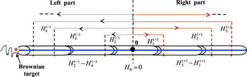
In the above techniques, we ask ourselves, how the Coordinated search technique minimizes the expected search time although the searchers return to the origin and one of them is waiting for the other?. The advanced technology can save this lost time without returning any searcher to the origin. Thus, the primary concern of this paper lies in the Coordinated search technique which allows two unit-speed searchers starting at the origin point seek for a Brownian target without returning to the origin. The first searcher searches the right part of the real line towards to $+\mathrm{\infty }$ and the other searcher searches the left part towards to $-\mathrm{\infty }$. We aim to show there exists a finite search plan that and calculates the expected value of the first meeting time between the searcher and the target.

This paper is organized as follows: Section 2 discusses the assumptions which modelling the search problem for a Brownian target. In Section 3 we determine the conditions that make the search plan be finite. We calculate the expected value of the first meeting time between the searcher and the target, in Section 4. Section 5 gives an example with numerical results that can show the effectiveness of this model. Finally, the paper concludes with a discussion of the results and directions for future research.

2. Problem formulation

In the well-known linear search problem, the searcher does step number $n$ after repeating all previous steps, why? This wastes the detection time (cost) (see Beck [21,22]). Here we aim to reduce this cost by presenting a new search model. The idea of this model is inspired by the coordinated search technique. Using the connection technology methods, any one of the searcher should not repeat any steps as in Reyniers [1,2].

2.1. The searching framework

The space of search: The search space is an axis of a cylinder (a real line $L$ ).

The target: The target is assumed to move randomly on the real line according to the Brownian motion $\left\{B\right(t),t\ge 0\}.$ The initial position of the target is unknown but the searchers know its probability distribution (the probability distribution of the target is given at time 0, and the process $\left\{B\right(t),t\ge 0\}$ which controls the target’s motion).

The means of search: We have two searchers $S_1\text{and}{S}_2$ start together looking for the target from the origin. The searcher $S_1$ searches in the right part and $S_2$ in the left part of the real line. They do not return to the origin after searching successively common distances until the target is found. This provides almost half the cost which had been obtained by Reyniers [1,2].

The searcher $S_{\ell },\ell =1,2$ would conduct its search in the following manner: Start at $H_0=0$ and go to the right (left) as far as $H_1^{(+)}\left(H_2^{(-)}\right)$. Then, use the wireless communication methods to tell the other searcher if the target is found or not. Retrace the steps again at the point $H_1^{(+)}\left(H_2^{(-)}\right)$ to explore the right (left) part of $H_1^{(+)}\left(H_2^{(-)}\right)$ as far as $[H_3^{(+)}-H_1^{(+)}]\left(\right[H_2^{(-)}-H_4^{(-)}\left]\right)$ and so on, see Figure 1.

Figure 1 Coordinated search technique for finding a Brownian target.

The objective is to obtain the condition that makes the search plan be finite.

3. Existence of a finite search plan

The two searchers $S_1$ and $S_2$ are coordinating their search and following the search paths $\varphi :R^{+}\to R\text{and }\overline{\varphi }:R^{+}\to R,$ respectively, to detect the target, where, (1) $\begin{array}{rl}& |\varphi \left(t_1\right)-\varphi \left(t_2\right)|\le v^{(+)}|t_1-t_2{|}_{}{\mathrm{\&}}^{}|\overline{\varphi }\left(t_1\right)-\overline{\varphi }\left(t_2\right)|\\ & \le v^{(-)}|t_1-t_2|\mathrm{\forall }{t}_1,t_2\in R^{+}\end{array}$(1) and $v^{(+)}$, $v^{(-)}$ are the velocities of the searchers in the right and left part respectively. Let ${\theta }_{(+)},{\theta }_{(-)},{\lambda }_{(+)}$ and ${\lambda }_{(-)}$ are positive integer numbers greater than one. We introduce the sequences $\{G_i^{(+)}{\}}_{i\ge 1}$, $\{G_i^{(-)}{\}}_{i\ge 1}$, $\{H_i^{(+)}{\}}_{i\ge 1}$ and $\{H_i^{(-)}{\}}_{i\ge 1}$ (see El-Rayes et al. [23]) to obtain the distances which the searchers should do them as a function of ${\theta }_{(+)},{\theta }_{(-)},{\lambda }_{(+)}$ and ${\lambda }_{(-)}$. In this model the searchers do not return to the origin as in Figure 1 then we can define: $G_i^{(+)}={\lambda }_{(+)}({\theta }_{(+)}^i-1),G_i^{(-)}={\lambda }_{(-)}({\theta }_{(-)}^i-1).$ Also, there is no return time to the origin then the travelled distances at the time step $i$ are given by: $H_i^{(+)}=C^{(+)}(G_i^{(+)}+2){,}^{}{H}_i^{(-)}=C^{(-)}(G_i^{(-)}+2),$ in the right and left part of the real line, respectively. And, $C^{(+)}=\frac{{\varpi }^{(+)}({\theta }_{(+)}-1)}{({\theta }_{(+)}+1)}{,}^{}{C}^{(-)}=\frac{{\varpi }^{(-)}({\theta }_{(-)}-1)}{({\theta }_{(-)}+1)}$ , where ${\varpi }^{(+)}$, ${\varpi }^{(-)}$ are rational numbers.

Now, we can define the search paths as follows: in the right part, for any $t\in R^{+},$ if $G_{2i-3}^{(+)}\le t\le G_{2i-1}^{(+)}$, then: (2) $\varphi \left(t\right)=(H_{2i-1}^{(+)}-H_{2i-3}^{(+)})+(t-G_{2i-1}^{(+)})$(2)

In the left part, for any $t\in R^{+},$ if $G_{2i-2}^{(-)}\le t\le G_{2i}^{(-)}$, then: (3) $\overline{\varphi }\left(t\right)=-\left[\right(H_{2i}^{(-)}-H_{2i-2}^{(-)})+(t-G_{2i}^{(-)}\left)\right]$(3)

Assuming that the notations $\psi \left(G_{2i-1}^{(+)}\right)=B\left(G_{2i-1}^{(+)}\right)-C^{(+)}\left(G_{2i-1}^{(+)}\right)$, $\tilde{\psi }\left(G_{2i}^{(-)}\right)=B\left(G_{2i}^{(-)}\right)+C^{(-)}\left(G_{2i}^{(-)}\right)$ are held and $\tau$ is the first meeting between one of the searcher and the target where, $\tau =\text{inf { }t:\text{either }\varphi \left(t\right)=Z_0+B\left(t\right)\text{or }\overline{\varphi }\left(t\right)=Z_0+B\left(t\right)\},$ $Z_0$ is a random variable which represents the initial position of the target and independent with $B\left(t\right),t>0.$ In addition, we let the search plan be represented by $(\varphi ,\overline{\varphi })\in {\mathrm{\Phi }}_0$, where ${\mathrm{\Phi }}_0=\left\{\right(\varphi ,\overline{\varphi }):\varphi \in \mathrm{\Phi },\overline{\varphi }\in \overline{\mathrm{\Phi }}\}$.

Since, the probability density function can be described as a calendar for the continuity of the relative frequencies of the data in a given interval, because the sample space contains an infinite number of possible outcomes. Therefore, the probability of any certain value is equal to zero. Due to the occurrence of the first meeting time between one of the searchers and the Brownian target at one certain values (Legal values) $z\in Z$ on the given field $[0,\mathrm{\infty }[$ or $]-\mathrm{\infty },0]$ have a known probability values greater than zero, then we need to define a new space (probability space). As a result, the integration will done on these legal and non-certain groups in an unconventional way. Thus, assume that the random variable that represents the position of the Brownian target is defined on a probability space $(\mathrm{\Omega },\mathrm{\Sigma },\gamma )$, where $\mathrm{\Omega }$ is the sample space of all possible meeting points, $\mathrm{\Sigma }$ is the σ- algebra (the collection of all events (mutually exclusive events) that show the position of the target at any time) and $\gamma$ is the probability measure which used as a measure of an integrator factor into $(\mathrm{\Omega },\mathrm{\Sigma },\gamma )$ in order to integration, but not the same way as a regular integration.

Theorem 3.1:

If $P(\tau >0)$ is a given initial probability of the first meeting time and ( $\varphi$ , $\overline{\varphi }$ ) $\in {\mathrm{\Phi }}_0$ , then the expectation $E\left(\tau \right)$ is finite if: ${\int }_0^{\mathrm{\infty }}{\sum }_{i=2}^{\mathrm{\infty }}{\theta }_{(+)}^{2i-2}p\left(\psi \right(G_{(2i-3)}^{(+)})>-z)\gamma \left(dz\right)$ and ${\int }_{-\mathrm{\infty }}^0{\sum }_{i=2}^{\mathrm{\infty }}{\theta }_{(-)}^{2i-2}p\left(\tilde{\psi }\right(G_{2i-2}^{(-)})<-z)\gamma \left(dz\right)$ are finite.

Proof:

The first meeting time between $S_1$ and the Brownian target ${\tau }_{\varphi }$ is a mutually exhaustive event with ${\tau }_{\overline{\varphi }}$ (the first meeting time between $S_2$ and the Brownian target). Hence, for any $i\ge 0$ we have: $p(\tau >t)=p({\tau }_{\varphi }>t_{}o{r}_{}{\tau }_{\overline{\varphi }}>t)=p({\tau }_{\varphi }>t)+p({\tau }_{\overline{\varphi }}>t)$ Thus, we can find: (4) $\begin{array}{rl}E\left(\tau \right)& =\underset{0}{\overset{\mathrm{\infty }}{\int }}P(\tau >t)\text{d}t\le \sum _{i=1}^{\mathrm{\infty }}\\ & \times \left[\underset{G_{2i-3}^{(+)}}{\overset{G_{2i-1}^{(+)}}{\int }}P({\tau }_{\varphi }>t)\text{d}t+\underset{G_{2i-2}^{(-)}}{\overset{G_{2i}^{(-)}}{\int }}P({\tau }_{\overline{\varphi }}>t)\text{d}t\right]\\ & \le \sum _{i=1}^{\mathrm{\infty }}\left[\right(G_{2i-1}^{(+)}-G_{2i-3}^{(+)}\left)P\right({\tau }_{\varphi }>G_{2i-3}^{(+)}\left)\right)\\ & +(G_{2i}^{(-)}-G_{2i-2}^{(-)})P({\tau }_{\overline{\varphi }}>G_{2i-2}^{(-)})]\\ & \le \sum _{i=1}^{\mathrm{\infty }}\left[{\lambda }_{(+)}\right({\theta }_{(+)}^{2i-1}-{\theta }_{(+)}^{2i-3}\left)P\right({\tau }_{\varphi }>G_{2i-3}^{(+)})\\ & +{\lambda }_{(-)}({\theta }_{(-)}^{2i}-{\theta }_{(-)}^{2i-2})P({\tau }_{\overline{\varphi }}>G_{2i-2}^{(-)})]\\ & ={\lambda }_{(+)}{\theta }_{(+)}P({\tau }_{\varphi }>0)+{\lambda }_{(+)}{\theta }_{(+)}({\theta }_{(+)}^2-1)\\ & \times \sum _{i=2}^{\mathrm{\infty }}{\theta }_{(+)}^{2i-2}P({\tau }_{\varphi }>G_{2i-3}^{(+)})\\ & +{\lambda }_{(-)}{\theta }_{(-)}P({\tau }_{\overline{\varphi }}>0)+{\lambda }_{(-)}{\theta }_{(-)}^2({\theta }_{(-)}^2-1)\\ & \times \sum _{i=2}^{\mathrm{\infty }}{\theta }_{(-)}^{2i-2}P({\tau }_{\overline{\varphi }}>G_{2i-2}^{(-)})\end{array}$(4)

But, $p({\tau }_{\varphi }>G_{2i-3}^{(+)})\le \underset{0}{\overset{\mathrm{\infty }}{\int }}p(Z_0+B(G_{2i-3}^{(+)})>H_{2i-3}^{(+)}|Z_0=z)\gamma \left(dz\right),i\ge 1$ using the notation $\psi \left(G_{(2i-3)}^{(+)}\right)=B\left(G_{(2i-3)}^{(+)}\right)-C^{(+)}\left(G_{(2i-3)}^{(+)}\right),$ we can get $\psi \left(G_{(2i-3)}^{(+)}\right)>-z$ (El-Hadidy et al. [24,25]), then $p({\tau }_{\varphi }>G_{2i-3}^{(+)})\le \underset{0}{\overset{\mathrm{\infty }}{\int }}p\left(\psi \right(G_{(2i-3)}^{(+)})>-z)\gamma \left(dz\right),$ and also $p({\tau }_{\overline{\varphi }}>G_{2i-2}^{(-)})\le \underset{-\mathrm{\infty }}{\overset{0}{\int }}p\left(\tilde{\psi }\right(G_{2i-2}^{(-)})<-z)\gamma \left(dz\right).$

Hence, $\begin{array}{rl}& E\left(\tau \right)=g+{\lambda }_{(+)}{\theta }_{(+)}({\theta }_{(+)}^2-1)\underset{0}{\overset{\mathrm{\infty }}{\int }}M\left(z\right)\gamma \left(dz\right)\\ & +{\lambda }_{(-)}{\theta }_{(-)}^2({\theta }_{(-)}^2-1)\underset{-\mathrm{\infty }}{\overset{0}{\int }}L\left(z\right)\gamma \left(dz\right),\end{array}$ where $g=({\lambda }_{(+)}{\theta }_{(+)}+{\lambda }_{(-)}{\theta }_{(-)})P(\tau >0)$, $P(\tau >0)$ is the given initial probability of the first meeting time and $M\left(z\right)={\sum }_{i=2}^{\mathrm{\infty }}{\theta }_{(+)}^{2i-2}p\left(\psi \right(G_{(2i-3)}^{(+)})>-z)$ and $L\left(z\right)={\sum }_{i=2}^{\mathrm{\infty }}{\theta }_{(-)}^{2i-2}p\left(\tilde{\psi }\right(G_{2i-2}^{(-)})<-z)$ Thus, $E\left(\tau \right)$ is finite if : ${\int }_0^{\mathrm{\infty }}M\left(z\right)\gamma \left(dz\right)$ and ${\int }_{-\mathrm{\infty }}^{0}L\left(z\right)\gamma \left(dz\right)$ are finite.

It is clear that the expected value of the first meeting time $E\left(\tau \right)$ is smaller than the expected value of the first meeting time which has been obtained by El-Rayes et al. [23] where $\psi \left(G_{(2i-3)}^{(+)}\right)<<\psi \left(G_{(2i-1)}\right)$ and $\tilde{\psi }\left(G_{2i-2}^{(-)}\right)<<\tilde{\psi }\left(G_{2i}\right)$ because in El-Rayes et al. [23] and El-Hadidy et al. [24,25] the searchers repeat the searched distances many times tend to infinity in both sides of the real line. Thus, the model which studied here is more effective and applicable more than by the other models which were presented before by Reyniers [1,2], El-Rayes et al. [23] and El-Hadidy et al. [24,25]. To make this model more effective we want to get some conditions as in the following Theorem 3.2.

Theorem 3.2.

The chosen search plan should satisfies $M\left(z\right)\le \tilde{M}\left(|z|\right)$ and $L\left(z\right)\le \tilde{L}\left(|z|\right)$ , where $\tilde{M}\left(|z|\right)$ and $\tilde{L}\left(|z|\right)$ are linear functions.

Proof:

We shall prove the theorem for $M\left(|z|\right)$ and the other case can be proved by similar way. If $z\le 0$, then $M\left(z\right)\le M\left(0\right)$ but for $z>0$ we get $M\left(0\right)={\sum }_{i=2}^{\mathrm{\infty }}{\theta }_{(+)}^{2i-2}p\left(\psi \right(G_{(2i-1)}^{(+)})>0)$ . Consequently, (5) $M\left(z\right)=M\left(0\right)+\sum _{i=2}^{\mathrm{\infty }}{\theta }_{(+)}^{2i-2}p\left(\psi \right(G_{(2i-1)}^{(+)})\le 0)$(5)

Since the target starts its motion from a random point $z$ on the real line with drift $\mu$ and variance ${\sigma }^2,$ then for any $t\ge G_{2i-1}^{(+)}>0$ we have $\begin{array}{rl}& p\left(B\right(t)\ge \alpha t)\le p\left(B\right(G_{(2i-1)}^{(+)})\ge \alpha G_{(2i-1)}^{(+)})\\ & =p\left(\sigma \sqrt{G_{(2i-1)}^{(+)}}Z+\mu G_{(2i-1)}^{(+)}\ge \alpha G_{(2i-1)}^{(+)}\right),\end{array}$ where $\alpha$ is constant. This leads to, (6) $\begin{array}{rl}& p\left(Z\ge \frac{(\alpha -\mu )G_{(2i-1)}^{(+)}}{\sigma \sqrt{G_{(2i-1)}^{(+)}}}\right)=\underset{k}{\overset{\mathrm{\infty }}{\int }}\frac{1}{\sqrt{2\pi }}{e}^{-\frac{z^2}{2}}\text{d}z\\ & =\underset{0}{\overset{\mathrm{\infty }}{\int }}\frac{1}{\sqrt{2\pi }}{e}^{-\frac{{(x+k)}^2}{2}}\text{d}x\le \frac{1}{2}{\epsilon }^{G_{(2i-1)}^{(+)}},\end{array}$(6) where $k=\frac{(\alpha -\mu )G_{(2i-1)}^{(+)}}{\sigma \sqrt{G_{(2i-1)}^{(+)}}}$. Also, in the left part of the real line we can get, $p\left(Z<\frac{(\alpha -\mu )G_{(2i-2)}^{(-)}}{\sigma \sqrt{G_{(2i-2)}^{(-)}}}\right)\le 1-\frac{1}{2}{\epsilon }^{G_{(2i-2)}^{(-)}}.$ In (5) we have, $M\left(0\right)<\sum _{i=2}^{\mathrm{\infty }}{\theta }_{(+)}^{2i-2}{\epsilon }^{G_{(2i-1)}^{(+)}}),\begin{array}{ccc}& & 0<\epsilon <1\end{array}$ where $\psi \left(G_{2i-1}^{(+)}\right)=B\left(G_{2i-1}^{(+)}\right)-C^{(+)}\left(G_{2i-1}^{(+)}\right).$

In addition, for any two positions $z_2\le z_1$ of the Brownian target we have the probability, $p(z_2\le B(t)\le z_1)\le p(z_2\le B(G_{2i-1}^{(+)})\le z_1)$ is non-increasing with time $G_{2i-1}^{(+)}$ , where $t\ge G_{2i-1}^{(+)}\ge max\left(\frac{z_1}{\mu },\frac{z_2}{\mu }\right)$ because, $\begin{array}{rl}& p(z_2\le B(G_{2i-1}^{(+)})\le z_1)\\ & =p\left(z_2\le \sigma \sqrt{G_{(2i-1)}^{(+)}})Z+\mu G_{(2i-1)}^{(+)}\le z_1\right)\\ & =p\left(\frac{z_2-\mu G_{(2i-1)}^{(+)}}{\sigma \sqrt{G_{(2i-1)}^{(+)}}}\le Z\le \frac{z_1-\mu G_{(2i-1)}^{(+)}}{\sigma \sqrt{G_{(2i-1)}^{(+)}}}\right).\end{array}$ If $\mu <0$ then $\begin{array}{rl}& \frac{z_2-\mu G_{(2i-1)}^{(+)}}{\sigma \sqrt{G_{(2i-1)}^{(+)}}}\ge 0{,}^{}\frac{d}{d{G}_{(2i-1)}^{(+)}}\left(\frac{z_2-\mu G_{(2i-1)}^{(+)}}{\sigma \sqrt{G_{(2i-1)}^{(+)}}}\right)\ge 0,\\ & \frac{z_1-\mu G_{(2i-1)}^{(+)}}{\sigma \sqrt{G_{(2i-1)}^{(+)}}}\le 0\text{and}\frac{d}{d{G}_{(2i-1)}^{(+)}}\left(\frac{z_1-\mu G_{(2i-1)}^{(+)}}{\sigma \sqrt{G_{(2i-1)}^{(+)}}}\right)\le 0.\end{array}$ This leads to the probability $p(z_2\le B(G_{2i-1}^{(+)})\le z_1)$ be a non-increasing.

Consider that $\psi \left(n\right)=\sum _{i=1}^n{y}_i,$ where $\{y_i{\}}_{i\ge 1}$ is a sequence of independent identically distributed random variables and $y_i\sim N(\mu -\alpha ,{\sigma }^2)$. We define the following: $d_n=G_{2n+1}^{(+)}={\lambda }_{(+)}({\theta }_{(+)}^{2n+1}-1)$ and $U(j,j+1)={\sum }_{n=1}^{\mathrm{\infty }}p[-(j+1)<\psi (n)\le -j]$. We choose $d_m=max(0,\frac{z}{\mu })$ and $a\left(n\right)=p[-z<\psi (n)\le 0]={\sum }_{j=1}^{|z|}p[-(j+1)<\psi (n)\le -j]$. Thus, if $n>d_m$ and since $p(z_2\le B(G_{2i-1}^{(+)})\le z_1)$ is non-increasing with time $G_{2i-1}^{(+)},$ then we have $a\left(n\right)$ is non-increasing. Thus, $M\left(z\right)-M\left(0\right)={\sum }_{n=1}^m{\theta }_{(+)}^{2n+1}a\left(d_n\right)+\alpha {\sum }_{n=m+1}^{\mathrm{\infty }}(d_n-d_{n-1})a\left(d_n\right)$ and by applying Lemma 1 in El-Hadidy et al. [24,25] we get: $M\left(z\right)-M\left(0\right)\le {\sum }_{n=1}^m{\theta }_{(+)}^{2n+1}+\alpha {\sum }_{n=d_m}^{\mathrm{\infty }}a\left(n\right)\le d_m+{\lambda }_{(+)}(1-{\theta }_{(+)}^{})+{\sum }_{j=0}^{|z|}U(j,j+1)$.

Since, $\psi \left(n\right)={\sum }_{i=1}^n{y}_i$ and $y_i\sim N(\mu -\alpha ,{\sigma }^2)$ then $U(j,j+1)$ satisfies the renewal theorem (see Feller [26]). Hence, $U(j,j+1)$ is bounded $\mathrm{\forall }j$ by a constant. This leads to $M\left(z\right)\le M\left(0\right)+M_1+M_1(|z)|=\tilde{M}(|z|).$ Similarly, one can show that $L\left(z\right)\le \tilde{L}\left(|z|\right)$ in the right part.

The necessary and sufficient conditions, that shows the existence of a finite search plan, are equivalent to the condition $E|Z_0|<\mathrm{\infty }$, that is, sufficient from the direct consequence of Theorems 3.1, 3.2 and the following Theorem 3.3.

Theorem 3.3:

If there exists a finite search plan ( $\varphi$ , $\overline{\varphi }$ ) $\in {\mathrm{\Phi }}_o$ , then $E|Z_o|$ is finite.

Proof:

See El-Hadidy et al. [24].

4. Calculating $E\left(\tau \right)$

It is known that the Brownian motion is a limit of the simple Random Walk which has a Markov property. In addition, the Brownian motion is interpreted based on the Normal distribution. Therefore, we can exploit this fact to calculate $E\left(\tau \right)$ depending on the probability of meeting the target at the time $G_{2i-1}^{(+)}$ provided with the probability of meeting it at the time $G_{2i-3}^{(+)}$ as in the following Theorem 4.1.

Theorem 4.1:

The expected value of the first meeting time for the Brownian target is given by: (7) $\begin{array}{rl}& E\left(\tau \right)\le {\lambda }_{(+)}{\theta }_{(+)}+{\lambda }_{(-)}{\theta }_{(-)}+{\lambda }_{(+)}{\theta }_{(+)}({\theta }_{(+)}^2-1)\\ & \times \sum _{i=2}^{\mathrm{\infty }}{\theta }_{(+)}^{2i-2}{\int }_0^{\mathrm{\infty }}{\int }_{-\mathrm{\infty }}^{H_{2i-3}^{(+)}-z}[1-\mathrm{\Phi }(G_{2i-5}^{(+)}-z\left)\right]d\\ & \mathrm{\Phi }(G_{2i-5}^{(+)}-z)\gamma \left(dz\right)\\ & +{\lambda }_{(-)}{\theta }_{(-)}^2({\theta }_{(-)}^2-1)\sum _{i=2}^{\mathrm{\infty }}{\theta }_{(-)}^{2i-2}\underset{-\mathrm{\infty }}{\overset{0}{\int }}\underset{-\mathrm{\infty }}{\overset{H_{2i-2}^{(-)}+z}{\int }}\\ & \mathrm{\Phi }(G_{2i-4}^{(-)}+z)d\mathrm{\Phi }(G_{2i-4}^{(-)}+z)\gamma \left(dz\right)\end{array}$(7) where $\mathrm{\Phi }(G_{2i-5}^{(+)}-z)$ and $\mathrm{\Phi }(G_{2i-4}^{(-)}+z)$ are the distribution functions of the Normal random variables $(G_{2i-5}^{(+)}-z)\sim N(0,(G_{2i-3}^{(+)}-G_{2i-5}^{(+)}\left)\right)$ and $(G_{2i-4}^{(-)}+z)\sim N(0,(G_{2i-2}^{(-)}-G_{2i-4}^{(-)}\left)\right)$ , respectively.

Proof:

By using the knowing initial probability $P(\tau >0)$ in (4), we get: (8) $\begin{array}{rl}& E\left(\tau \right)\le ({\lambda }_{(+)}{\theta }_{(+)}+{\lambda }_{(-)}{\theta }_{(-)})P(\tau >0)\\ & +{\lambda }_{(+)}{\theta }_{(+)}({\theta }_{(+)}^2-1)\\ & \sum _{i=2}^{\mathrm{\infty }}{\theta }_{(+)}^{2i-2}P({\tau }_{\varphi }>G_{2i-3}^{(+)}))+{\lambda }_{(-)}{\theta }_{(-)}^2({\theta }_{(-)}^2-1)\\ & \times \sum _{i=2}^{\mathrm{\infty }}{\theta }_{(-)}^{2i-2}P({\tau }_{\overline{\varphi }}>(G_{2i}^{(-)}-G_{2i-2}^{(-)}\left)\right)\end{array}$(8) and since, $p({\tau }_{\varphi }>(G_{2i-3}^{(+)})\le {\int }_0^{\mathrm{\infty }}p(Z_0+B\left(G_{2i-3}^{(+)}\right)>\left(H_{2i-3}^{(+)}\right)|Z_0=z\left)\gamma \right(dz)$ we can find that: (9) $\begin{array}{rl}& p\left(Z_0+B\left(G_{2i-3}^{(+)}\right)>H_{2i-3}^{(+)}|Z_0=z\right)=p\left(\right(B\left(G_{2i-3}^{(+)}\right)\\ & >(H_{2i-3}^{(+)}-z)=1-p\left(B\right(G_{2i-3}^{(+)}\le (H_{2i-3}^{(+)}-z))\end{array}$(9) It is known that for the times $t,s$ the random variable $B\left(t\right)-B\left(s\right)$ has a normal distribution with mean 0 and variance $t-s$ where $s<t.$ Thus, we can get: $\begin{array}{rl}& p\left(B\right(G_{2i-3}^{(+)})\le (H_{2i-3}^{(+)}-z\left)\right)\le \underset{-\mathrm{\infty }}{\overset{\mathrm{\infty }}{\int }}p\left(B\right(G_{2i-5}^{(+)})\\ & \le (H_{2i-5}^{(+)}-z),\left[B\right(G_{2i-3}^{(+)})+B(G_{2i-5}^{(+)})-B(G_{2i-5}^{(+)}\left)\right]\\ & \le (H_{2i-5}^{(+)}-z)|B\left(G_{2i-5}^{(+)}\right)=(G_{2i-5}^{(+)}-z))\\ & \times \frac{1}{(G_{2i-3}^{(+)}-G_{2i-5}^{(+)})\sqrt{2\pi }}{e}^{-\frac{1}{2}{\left(\frac{G_{2i-5}^{(+)}-z}{(G_{2i-3}^{(+)}-G_{2i-5}^{(+)})}\right)}^2}\\ & \times d(G_{2i-5}^{(+)}-z)\\ & =\underset{-\mathrm{\infty }}{\overset{\mathrm{\infty }}{\int }}p(\left[B\right(G_{2i-3}^{(+)})+B(G_{2i-5}^{(+)}\left)\right]-B\left(G_{2i-5}^{(+)}\right)\\ & \le (H_{2i-5}^{(+)}-z)|B\left(G_{2i-5}^{(+)}\right)=(G_{2i-5}^{(+)}-z))\\ & \times \frac{1}{(G_{2i-3}^{(+)}-G_{2i-5}^{(+)})\sqrt{2\pi }}{e}^{-\frac{1}{2}{\left(\frac{G_{2i-5}^{(+)}-z}{(G_{2i-3}^{(+)}-G_{2i-5}^{(+)})}\right)}^2}\\ & \times d(G_{2i-5}^{(+)}-z)\end{array}$ (see Kelbaner [27]). Since the first meeting is not done at the time $t=G_{2i-5}^{(+)}$, then $\begin{array}{rl}& p\left(B\right(G_{2i-3}^{(+)}\le (H_{2i-3}^{(+)}-z))=\underset{-\mathrm{\infty }}{\overset{H_{2i-3}^{(+)}-z}{\int }}p(\left[\right(B\left(G_{2i-3}^{(+)}\right)\\ & \le (H_{2i-3}^{(+)}-z)]-[\left(B\right(G_{2i-5}^{(+)})\le (H_{2i-5}^{(+)})-z)]\\ & \le -(G_{2i-5}^{(+)}-z))\\ & \times \frac{1}{(G_{2i-3}^{(+)}-G_{2i-5}^{(+)})\sqrt{2\pi }}{e}^{-\frac{1}{2}{\left(\frac{G_{2i-5}^{(+)}-z}{(G_{2i-3}^{(+)}-G_{2i-5}^{(+)})}\right)}^2}\\ & \times d(G_{2i-5}^{(+)}-z)\\ & =\underset{-\mathrm{\infty }}{\overset{H_{2i-3}^{(+)}-z}{\int }}\mathrm{\Phi }(-(G_{2i-5}^{(+)}-z\left)d\mathrm{\Phi }\right(G_{2i-5}^{(+)}-z)\\ & =\underset{-\mathrm{\infty }}{\overset{H_{2i-3}^{(+)}-z}{\int }}[1-\mathrm{\Phi }(G_{2i-5}^{(+)}-z\left)\right]d\mathrm{\Phi }(G_{2i-5}^{(+)}-z),\end{array}$ where $\mathrm{\Phi }(G_{2i-5}^{(+)}-z)$ is the distribution function of the Normal random variable $(G_{2i-5}^{(+)}-z)\sim N(0,(G_{2i-3}^{(+)}-G_{2i-5}^{(+)}\left)\right).$ Similarly, we can calculate the probability: $\begin{array}{rl}& p(Z_0+B(G_{2i-2}^{(-)})<H_{2i-2}^{(-)}|Z_0=z)\\ & =p\left(B\right(G_{2i-2}^{(-)})-(H_{2i-2}^{(-)}+z)<0)\\ & =\underset{-\mathrm{\infty }}{\overset{H_{2i-2}^{(-)}+z}{\int }}\mathrm{\Phi }(G_{2i-2}^{(-)}+z)d\mathrm{\Phi }(G_{2i-2}^{(-)}+z)\end{array}$

Since the target starts its motion from a random point $z$, then we can consider that $P(\tau >0)=1$. Thus, in (8) we can get the approximate value of $E\left(\tau \right)$ as follows: $\begin{array}{rl}E\left(\tau \right)\le & {\lambda }_{(+)}{\theta }_{(+)}+{\lambda }_{(-)}{\theta }_{(-)}+{\lambda }_{(+)}{\theta }_{(+)}({\theta }_{(+)}^2-1)\\ & \sum _{i=2}^{\mathrm{\infty }}{\theta }_{(+)}^{2i-2}\underset{0}{\overset{\mathrm{\infty }}{\int }}\underset{-\mathrm{\infty }}{\overset{H_{2i-3}^{(+)}-z}{\int }}{[1-\mathrm{\Phi }(G_{2i-5}^{(+)}-z\left)\right]}^{}d\\ & \mathrm{\Phi }(G_{2i-5}^{(+)}-z)\gamma \left(dz\right)\\ & +{\lambda }_{(-)}{\theta }_{(-)}^2({\theta }_{(-)}^2-1)\sum _{i=2}^{\mathrm{\infty }}{\theta }_{(-)}^{2i-2}\underset{-\mathrm{\infty }}{\overset{0}{\int }}\underset{-\mathrm{\infty }}{\overset{H_{2i-2}^{(-)}+z}{\int }}\\ & \mathrm{\Phi }{(G_{2i-4}^{(-)}+z)}^{}d\mathrm{\Phi }(G_{2i-4}^{(-)}+z)\gamma \left(dz\right)\end{array}$

Since, ${\int }_{-\mathrm{\infty }}^{H_{2i-3}^{(+)}-z}{[1-\mathrm{\Phi }(G_{2i-5}^{(+)}-z\left)\right]}^{}d\mathrm{\Phi }(G_{2i-5}^{(+)}-z)={\int }_{-\mathrm{\infty }}^{H_{2i-3}^{(+)}-z}d\mathrm{\Phi }(G_{2i-5}^{(+)}-z)-{\int }_{-\mathrm{\infty }}^{H_{2i-3}^{(+)}-z}\mathrm{\Phi }(G_{2i-5}^{(+)}-z)d\mathrm{\Phi }(G_{2i-5}^{(+)}-z)$ and if we have $X\sim N(0,{\sigma }^2)$, then ${\int }_{-\mathrm{\infty }}^{0}d\mathrm{\Phi }\left(x\right)=\frac{1}{2}$. Consequently, one can get $\frac{1}{2}<{\int }_{-\mathrm{\infty }}^{H_{2i-3}^{(+)}-z}d\mathrm{\Phi }(G_{2i-5}^{(+)}-z)<1$ where $H_{2i-3}^{(+)}-z>0$. In addition, ${\int }_{-\mathrm{\infty }}^0\mathrm{\Phi }\left(x\right)d\mathrm{\Phi }\left(x\right)={\int }_0^{1/2}xdx=\frac{1}{8}<\frac{1}{2}$ thus it is easily to conclude that $0<{\int }_{-\mathrm{\infty }}^{H_{2i-3}^{(+)}-z}\mathrm{\Phi }{(G_{2i-5}^{(+)}-z)}^{}d\mathrm{\Phi }(G_{2i-5}^{(+)}-z)<\frac{1}{2}$. This can show that the integrals in (7), are indeed finite where the target is not evading the searching process.

5. Application

Assuming a rocket (target) fires from a random point (rocket launcher carries on lorry’s enemy) on the road (real line) and moves with a Brownian motion. The approximated value of the expected value of the first meeting time between one of the searchers and the rocket depends on the values of the distances that the each searcher should do them. Since, ${\int }_{-\mathrm{\infty }}^{H_{2i-3}^{(+)}-z}\mathrm{\Phi }(G_{2i-5}^{(+)}-z)d\mathrm{\Phi }(G_{2i-5}^{(+)}-z)<\frac{1}{2}$ and $\frac{1}{2}<{\int }_{-\mathrm{\infty }}^{H_{2i-3}^{(+)}-z}d\mathrm{\Phi }(G_{2i-5}^{(+)}-z)<1$ then we can let ${\int }_{-\mathrm{\infty }}^{H_{2i-3}^{(+)}-z}[1-\mathrm{\Phi }(G_{2i-5}^{(+)}-z\left)\right]d\mathrm{\Phi }(G_{2i-5}^{(+)}-z)={\rho }_{2i-3}^{(+)}$ and ${\int }_{-\mathrm{\infty }}^{H_{2i-2}^{(-)}+z}\mathrm{\Phi }(G_{2i-4}^{(-)}+z)d\mathrm{\Phi }(G_{2i-4}^{(-)}+z)={\rho }_{2i-2}^{(-)},$ where $0<{\rho }_{2i-3}^{(+)}<1$ and $0<{\rho }_{2i-2}^{(-)}<\frac{1}{2}$ such that ${\rho }_{2i-2}^{(-)}+{\rho }_{2i-3}^{(+)}=1$. Thus, let ${\theta }_{(+)}=1.1{,}_{}{\theta }_{(-)}=1.2{,}_{}{\lambda }_{(+)}=1.01$ and ${\lambda }_{(-)}=1.05$ then by compensation in (7) we get: $\begin{array}{rl}& E\left(\tau \right)<2.37+\left(0.255\right)\sum _{i=2}^{\mathrm{\infty }}{\left(1.1\right)}^{2i-2}\underset{0}{\overset{\mathrm{\infty }}{\int }}{\rho }_{2i-3}^{(+)}\gamma (dz)\\ & +\left(0.665\right)\sum _{i=2}^{\mathrm{\infty }}(1.2{)}^{2i-2}\underset{-\mathrm{\infty }}{\overset{0}{\int }}{\rho }_{2i-2}^{(-)}\gamma \left(dz\right),\end{array}$ where $0<{\rho }_{2i-3}^{(+)}\le 1$ and $0<{\rho }_{2i-2}^{(-)}<\frac{1}{2}$. From probability measure theory one can get, $\begin{array}{rl}& E\left(\tau \right)<2.37+\left(0.255\right)\left(\underset{0}{\overset{\mathrm{\infty }}{\int }}\gamma (dz)\right)\\ & \times \left(\sum _{i=2}^{\mathrm{\infty }}{\left(1.1\right)}^{2i-2}{\rho }_{2i-3}^{(+)}\right)\\ & +\left(0.665\right)\left(\underset{-\mathrm{\infty }}{\overset{0}{\int }}\gamma \left(dz\right)\right)\left(\sum _{i=2}^{\mathrm{\infty }}{\left(1.2\right)}^{2i-2}{\rho }_{2i-2}^{(-)}\right).\end{array}$

Also, we know that ${\int }_{-\mathrm{\infty }}^0\gamma \left(dz\right)+{\int }_0^{\mathrm{\infty }}\gamma \left(dz\right)=1$, then if we let ${\int }_{-\mathrm{\infty }}^0\gamma \left(dz\right)=\kappa$ then we have ${\int }_0^{\mathrm{\infty }}\gamma \left(dz\right)=1-\kappa .$ Consequently, $\begin{array}{rl}& E\left(\tau \right)<2.37+\left(0.255\right)\kappa \left(\sum _{i=2}^{\mathrm{\infty }}{\left(1.1\right)}^{2i-2}{\rho }_{2i-3}^{(+)}\right)\\ & +\left(0.665\right)(1-\kappa )\left(\sum _{i=2}^{\mathrm{\infty }}{\left(1.2\right)}^{2i-2}{\rho }_{2i-2}^{(-)}\right).\end{array}$ After knowing the number of steps, one of the searcher will meet the target. Thus, if the target will be met after step number 10, then we have, (10) $\begin{array}{rl}& E\left(\tau \right)<2.37+\left(0.255\right)\kappa \left(\sum _{i=2}^{10}{\left(1.1\right)}^{2i-2}{\rho }_{2i-3}^{(+)}\right)\\ & +\left(0.665\right)(1-\kappa )\left(\sum _{i=2}^{10}{\left(1.2\right)}^{2i-2}{\rho }_{2i-2}^{(-)}\right).\end{array}$(10)

Let $\kappa =0.7$ and let the different values of ${\rho }_{2i-3}^{(+)}$ and ${\rho }_{2i-2}^{(-)}$ are given by Table 1.

Table 1. Different values of ${\rho }_{2i-3}^{(+)}$ and ${\rho }_{2i-2}^{(-)}$.

$i$	2	3	4	5	6	7	8	9	10
${\rho }_{2i-3}^{(+)}$	0.55	0.6	0.65	0.7	0.75	0.8	0.85	0.9	0.95
${\rho }_{2i-2}^{(-)}$	0.45	0.4	0.35	0.3	0.25	0.2	0.15	0.1	0.05

In (11) we find that the expected cost of the first meeting time between one of the searchers and the Brownian target is less than $\text{ 22}\text{.9148}$ unit of time.

6. Conclusion

The coordinated linear search technique for a Brownian target on the real line has been presented, where the target initial position is given by a random variable $Z_0$. We found the conditions that make the expected value of the first meeting time between one of the searchers and the target is finite in Theorem 3.1 based on the continuity of the search plan. In Theorems 3.2, we presented that The chosen search plan should satisfies the conditions ${\sum }_{i=2}^{\mathrm{\infty }}{\theta }_{(+)}^{2i-2}p\left(\psi \right(G_{(2i-3)}^{(+)})>-z)\le \tilde{M}\left(|z|\right)$ and ${\sum }_{i=2}^{\mathrm{\infty }}{\theta }_{(-)}^{2i-2}p\left(\tilde{\psi }\right(G_{2i-2}^{(-)})<-z)\le \tilde{L}\left(|z|\right)$, where $\tilde{M}\left(|z|\right)$ and $\tilde{L}\left(|z|\right)$ are linear functions. We calculated the approximated value for the expected value of the first meeting time. The effectiveness of this model is illustrated using a real-life application.

In future research, it seems that the proposed model will be extendible to the multiple searchers case by considering the combinations of movement of multiple targets.

Disclosure statement

No potential conflict of interest was reported by the authors.

ORCID

Alaa Awad Alzulaibani http://orcid.org/0000-0003-3742-8003

References

- Reyniers DJ. Coordinated search for an object on the line. Eur J Oper Res. 1996;95(3):663–670. doi: 10.1016/S0377-2217(96)00314-1
- Reyniers DJ. Coordinated two searchers for an object hidden on an interval. J Oper Res Soc. 1995;46(11):1386–1392. doi: 10.1057/jors.1995.186
- Mohamed A, Abou-Gabal H, El-Hadidy M. Coordinated search for a randomly located target on the plane. Eur J Pure Appl Math. 2009;2(1):97–111.
- Mohamed A, Fergany H, El-Hadidy M. On the coordinated search problem on the plane. Istan Univ J Sch Busin Admin. 2012;41(1):80–102.
- Kassem M, El-Hadidy M. Optimal Multiplicative Bayesian search for a lost target. Appl Math Comput. 2014;247:795–802.
- El-Hadidy MA. Optimal Spiral search plan for a randomly located target in the plane. Int J Oper Res. 2015;22(4):454–465. doi: 10.1504/IJOR.2015.068561
- El-Hadidy MA. Optimal searching for a Helix target motion. Sci China Math. 2015;58(4):749–762. doi: 10.1007/s11425-014-4864-5
- Mohamed A, Kassem M, El-Hadidy M. M-States search problem for a lost target with multiple sensors. Int J Math Oper Res. 2017;10(1):104–135. doi: 10.1504/IJMOR.2017.080747
- Mohamed AA, Abou Gabal HM, El-Hadidy MA. Random search in a bounded area. Int J Math Oper Res. 2017;10(2):137–149. doi: 10.1504/IJMOR.2017.081921
- El-Hadidy M. Fuzzy optimal search plan for N-Dimensional randomly moving target. Int J Computational Methods. 2016;13(6):1650038 (38 pages). doi: 10.1142/S0219876216500389
- El-Hadidy M. On Maximum Discounted Effort Reward search problem. Asia-Pacific J Oper Res. 2016;33(3):1650019 (30 pages). doi: 10.1142/S0217595916500196
- El-Hadidy M. On the existence of a finite linear search plan with random distances and velocities for a One-Dimensional Brownian target. Int J Oper Res. 2017. http://www.inderscience.com/info/ingeneral/forthcoming.php?jcode=ijor
- El-Hadidy MA. Existence of finite Parbolic Spiral search plan for a Brownian target. Int J Oper Res. 2017. http://www.inderscience.com/info/ingeneral/forthcoming.php?jcode;otherinfo>=ijor/otherinfo>.
- Kagan E, Ben-Gal I. Search and Foraging: Individual motion and Swarm Dynamics. Boca Raton (FL): CRC Press; 2015.
- Guerrier C, Holcman D. Brownian search for targets hidden in cusp-like pockets: Progress and Applications. Eur Phy J Spec Top. 2014;223(14):3273–3285. doi: 10.1140/epjst/e2014-02332-6
- Palyulin VV, Chechkin AV, Metzler R. Space-fractional Fokker–Planck equation and optimization of random search processes in the presence of an external bias. J Stat Mech Theor Exp. 2014;11:P11031. doi: 10.1088/1742-5468/2014/11/P11031
- Radmard S, Croft E. Active target search for high dimensional robotic systems. Auton Robots. 2017;41(1):163–180. doi: 10.1007/s10514-015-9539-8
- Stone LD, Royset JO, Washburn AR. Optimal search for moving targets, part of the International Series in Operations research & Management Science book series. Cham: Springer; 2016.
- El-Hadidy M, Abou-Gabal H. Coordinated search for a random Walk target motion. Fluctuation Noise Lett. 2018;17(1):1850002 (11 pages). doi: 10.1142/S0219477518500025
- Mohamed A, El-Hadidy M. Coordinated search for a conditionally deterministic target motion in the plane. Eur J Math Sci. 2013;2(3):272–295.
- Beck A. On the linear search problem. Israel J Math. 1964;2(4):221–228. doi: 10.1007/BF02759737
- Beck A. More on the linear search problem. Israel J Math. 1965;3(4):61–70. doi: 10.1007/BF02760028
- El-Rayes AB, Mohamed AA, Abou Gabal HM. Linear search for a brownian target motion. Acta Math Scientia J. 2003;23 (B)(3):321–327. doi: 10.1016/S0252-9602(17)30338-7
- Mohamed A, Kassem M, El-Hadidy M. Multiplicative linear search for a brownian target motion. Appli Math Model. 2011;35(9):4127–4139. doi: 10.1016/j.apm.2011.03.024
- El-Hadidy M. Searching for a d-dimensional Brownian target with multiple sensors. Int J Math Oper Res. 2016;9(3):279–301. doi: 10.1504/IJMOR.2016.10000114
- Feller W. An Introduction to probability theory and its applications. Vol II. New York: Wiley; 1966.
- Klebaner FC. Introduction to stochastic calculus with applications. London: Imperial College Press; 1998.