Internal truncated distributions: applications to Wiener process range distribution when deleting a minimum stochastic volatility interval from its domain

ABSTRACT

In this paper, we apply a new definition of truncated distribution “Internal Truncated Distribution” on the Wiener process range distribution to delete a few stochastic volatility intervals from its domain. A comprehensive treatment of the statistical properties of this distribution is presented. The usefulness of the proposed distribution is illustrated with the help of a real data set.

KEYWORDS:

• Internal truncated distribution
• Wiener process range distribution
• stochastic volatility
• reliability properties

MATHEMATICS SUBJECT CLASSIFICATION (2010):

• 60J65
• 60K40
• 62E10

1. Introduction

During the first three decades of the twentieth century, Norbert Wiener discovered a new stochastic process called Wiener process $\left\{W\right(t);t\ge 0\}$. Also, this process is called a standard Brownian motion. The Wiener process has a remarkable importance in the mathematical theory of finance, in particular, the Black–Schools option pricing model. We know that at any time interval $(0,T)$, the Wiener process range is the best random variable which illustrates the difference between the highest and lowest value of the sale price. This range is defined by $\tilde{R}\left(T\right)=\underset{(0,T)}{sup}W\left(t\right)-\underset{(0,T)}{inf}W\left(t\right)$, where $0<\tilde{r}<\mathrm{\infty }$ and $T>0.$ Early, Feller [1] used the method of images to derive the probability density function of this range. Recently, Withers and Nadarajah [2] gave an expansion for its cumulative distribution function and its quantiles. More recently, Teamah et al. [3] asked an interesting question, that is; what should be done if we need to find the new distribution of the stock price in the time interval $(0,T)$ and its value is sandwiched between two certain values $a,b$? Already, they answered the above question by using the truncation method on the Wiener process range distribution that was obtained by Feller [1]. Also, Teamah et al. [3] presented some statistical properties of this distribution including reliability properties, moments, stress-strength parameter, order statistics, Bonferroni curve, Lorenz curve and Gini's index.

The idea of the truncation method of any distribution is to delete a certain period from its random variable domain and then find its conditional distribution. The probability of the truncated part is distributed on the other part until the area under the new curve (curve after truncated) becomes equal to one. There are two kinds of truncation: (i) single truncation from one, left or right side of the domain and (ii) double truncation from both sides of the domain. In [4–8], some details about truncated distribution have been discussed.

Here, we have a more interesting question; that is; what happened for the Wiener range distribution if we want to delete some intervals which contain few stochastic volatility of the stock price? In other words, why we consider these intervals (which contain few stochastic volatility) for this distribution? In order to address this problem, we present a new definition called “multi-internal truncated distribution” to delete these intervals from the Wiener process range which has been obtained by Feller [1]. In this definition, we redistribute the probabilities of the truncation parts to the remaining parts. Another feature of this definition allows us to distribute these probabilities with different proportions to the remaining parts.

In this paper, we will present one internal truncated distribution of a Wiener process range (i.e. we want to delete one interval $[\alpha ,\beta ]$ from the range such that $0<r<\alpha$ and $\beta <r<\mathrm{\infty }$) and study comprehensive treatment of the statistical properties. The properties studied include reliability properties, moments, stress-strength parameter, Bonferroni curve, Lorenz curve and Gini's index. The difference between the one internal truncated distribution and distribution of a Wiener process range which has been obtained by Feller [1] are shown as in the given figures through this paper.

This paper is organized as follows. In Section 2, we present the definition of one internal truncated Wiener process range distribution. We discuss some statistical properties for one internal truncated distribution in Section 3. A data set application is presented in Section 4. Section 5 ends this paper with some concluding remarks and future works.

2. One internal truncated distribution of a Wiener process range

Sometimes, we need to delete some values of the domain of the stock price which is assumed to move randomly according to one dimensional Wiener process $\left\{W\right(t),t\in {\mathbb{R}}^{+}\}$, where $\mathbb{R}$⁺ is the set of real numbers, and $W\left(t\right)$ is a Wiener process on $(0,\mathrm{\infty })$ with the range $\tilde{R}\left(T\right)$ on the time interval $(0,T)$. This range is the difference between ${sup}_{(0,T)}W\left(t\right)$ and ${inf}_{(0,T)}W\left(t\right)$. Feller [1] gave the probability density function for the range of $W\left(t\right)$ which controls the target's motion as (1) $\begin{array}{rl}{f}_{\tilde{R}\left(T\right)}\left(\tilde{r}\right)& ={\left(\frac{2}{\pi }\right)}^{\frac{1}{2}}{\tilde{r}}^{-1}(2\pi {)}^{\frac{1}{2}}{\left(\frac{\tilde{r}{T}^{-\frac{1}{2}}}{2}\right)}^{-1}\\ & \times \sum _{k=1}^{\mathrm{\infty }}\exp \left[-\frac{{(2k-1)}^2{\pi }^2}{8}.{\left(\frac{\tilde{r}{T}^{-\frac{1}{2}}}{2}\right)}^{-2}\right],\end{array}$(1) where $0<\tilde{r}<\mathrm{\infty }$ and $T>0$ (see Figure 1).

Figure 1. Probability density function of $\tilde{R}\left(T\right)$.

In addition, Withers and Nadarajah [2] give its cumulative distribution function by (2) $\begin{array}{rl}{F}_{\tilde{R}\left(T\right)}\left(\tilde{r}\right)& =\sum _{k=1}^{\mathrm{\infty }}\left(\frac{8}{{(2k-1)}^2{\pi }^2}+\frac{8T}{{\tilde{r}}^2}\right)\\ & \exp \left[-\frac{{(2k-1)}^2{\pi }^{2}T}{2{\tilde{r}}^2}\right],\end{array}$(2)

In real life, we know that the value of the stock price in the time interval $(0,T)$ is sandwiched between two certain values $a,b$(see Figure 2). In this case, Teamah et al. [3] gave the distribution of this bounded range by make double truncation of (1) as (3) $h_{\widehat{\stackrel{~}{R}}\left(T\right)}\left(\widehat{\stackrel{~}{r}}\right)=\frac{\begin{array}{c}\left|\frac{T^{\frac{-1}{2}}}{2}\right|\sum _{k=1}^{\mathrm{\infty }}\left(\frac{8}{{(2k-1)}^2{\pi }^2}+8{\widehat{\stackrel{~}{r}}}^{-2}T\right)\\ e^{-\frac{{(2k-1)}^2{\pi }^2{\widehat{\stackrel{~}{r}}}^{-2}T}{2}}\end{array}}{\begin{array}{c}\sum _{k=1}^{\mathrm{\infty }}\left(\frac{8}{{(2k-1)}^2{\pi }^2}+8T{b}^{-2}\right)e^{-\frac{{(2k-1)}^2{\pi }^{2}T{b}^{-2}}{2}}\\ -\sum _{k=1}^{\mathrm{\infty }}\left(\frac{8}{{(2k-1)}^2{\pi }^2}+8T{a}^{-2}\right)e^{-\frac{{(2k-1)}^2{\pi }^{2}T{a}^{-2}}{2}}\end{array}},$(3) where $a<\widehat{\stackrel{~}{r}}<b$ and $T>0.$

Figure 2. Distribution function of $\tilde{R}\left(T\right)$.

In this work, we aim to delete some values from the domain of the range. These values show that there are no or few stochastic volatility. We are interested in the distribution of multi-internal truncated random variables which is defined by:

Definition 2.1:

Let $\tilde{R}\left(T\right)$ be a random variable with known probability density function, define $R\left(T\right)$ as a corresponding n-internal truncated of the random variable $\tilde{R}\left(T\right)$ with pdf $g_{R\left(T\right)}\left(r\right)$. Then, the probability density function of multi-internal of $\tilde{R}\left(T\right)$ is given by

$\begin{array}{rl}& g_{R\left(T\right)}\left(r\right)=\\ & \left\{\begin{array}{ll}\frac{f_{R\left(T\right)}\left(r\right)}{1-F_{R\left(T\right)}\left({\beta }_n\right)+\sum _{i=1}^n\left[F_{R\left(T\right)}\left({\alpha }_i\right)-F_{R\left(T\right)}\left({\beta }_{i-1}\right)\right]},& 0<r<\alpha ,\\ \frac{f_{R\left(T\right)}\left(r\right)}{1-F_{R\left(T\right)}\left({\beta }_n\right)+\sum _{i=1}^n\left[F_{R\left(T\right)}\left({\alpha }_i\right)-F_{R\left(T\right)}\left({\beta }_{i-1}\right)\right]},& {\beta }_1<r<{\alpha }_2,\\ \frac{f_{R\left(T\right)}\left(r\right)}{1-F_{R\left(T\right)}\left({\beta }_n\right)+\sum _{i=1}^n\left[F_{R\left(T\right)}\left({\alpha }_i\right)-F_{R\left(T\right)}\left({\beta }_{i-1}\right)\right]},& {\beta }_2<r<{\alpha }_3,\\ ⋮& ⋮\\ \frac{f_{R\left(T\right)}\left(r\right)}{1-F_{R\left(T\right)}\left({\beta }_n\right)+\sum _{i=1}^n\left[F_{R\left(T\right)}\left({\alpha }_i\right)-F_{R\left(T\right)}\left({\beta }_{i-1}\right)\right]},& {\beta }_{n-1}<r<{\alpha }_n,\\ \frac{f_{R\left(T\right)}\left(r\right)}{1-F_{R\left(T\right)}\left({\beta }_n\right)+\sum _{i=1}^n\left[F_{R\left(T\right)}\left({\alpha }_i\right)-F_{R\left(T\right)}\left({\beta }_{i-1}\right)\right]},& {\beta }_n<r<\mathrm{\infty },\end{array}\right.\end{array}$ where ${\beta }_0=-\mathrm{\infty }$.

The idea of the above definition has been drawn from the idea of left, right and double truncation which is studied in [9–11]. In our definition, we distribute the area under the probability curve on the remaining parts with equal proportions.

In our problem, we consider that the range has one interval that contains few stochastic volatility (there are very small changes in option price) and we need to truncate this interval. From Definition 2.1, we can do one internal truncation for (1). Consequently, we get

(4) $\begin{array}{rl}{g}_{R\left(T\right)}\left(r\right)& =\left\{\begin{array}{ll}\frac{f_{R\left(T\right)}\left(r\right)}{1-F_{R\left(T\right)}\left(\beta \right)+F_{R\left(T\right)}\left(\alpha \right)},& 0<r<\alpha ,\\ \frac{f_{R\left(T\right)}\left(r\right)}{1-F_{R\left(T\right)}\left(\beta \right)+F_{R\left(T\right)}\left(\alpha \right)},& \beta <r<\mathrm{\infty },\end{array}\right.\\ & =\left\{\begin{array}{ll}\frac{{\left(\frac{2}{\pi }\right)}^{\frac{1}{2}}{r}^{-1}{\left(2\pi \right)}^{\frac{1}{2}}{\left(\frac{r{T}^{-\frac{1}{2}}}{2}\right)}^{-1}\sum _{k=1}^{\mathrm{\infty }}\exp \left[-\frac{{(2k-1)}^2{\pi }^2}{8}.{\left(\frac{r{T}^{-\frac{1}{2}}}{2}\right)}^{-2}\right]}{1-\sum _{k=1}^{\mathrm{\infty }}\left(\frac{8}{{(2k-1)}^2{\pi }^2}+\frac{8T}{{\beta }^2}\right)\exp \left[-\frac{{(2k-1)}^2{\pi }^{2}T}{2{\beta }^2}\right]+\sum _{k=1}^{\mathrm{\infty }}\left(\frac{8}{{(2k-1)}^2{\pi }^2}+\frac{8T}{{\alpha }^2}\right)\exp \left[-\frac{{(2k-1)}^2{\pi }^{2}T}{2{\alpha }^2}\right]},& 0<r<\alpha ,\\ \frac{{\left(\frac{2}{\pi }\right)}^{\frac{1}{2}}{r}^{-1}{\left(2\pi \right)}^{\frac{1}{2}}{\left(\frac{r{T}^{-\frac{1}{2}}}{2}\right)}^{-1}\sum _{k=1}^{\mathrm{\infty }}\exp \left[-\frac{{(2k-1)}^2{\pi }^2}{8}.{\left(\frac{r{T}^{-\frac{1}{2}}}{2}\right)}^{-2}\right]}{1-\sum _{k=1}^{\mathrm{\infty }}\left(\frac{8}{{(2k-1)}^2{\pi }^2}+\frac{8T}{{\beta }^2}\right)\exp \left[-\frac{{(2k-1)}^2{\pi }^{2}T}{2{\beta }^2}\right]+\sum _{k=1}^{\mathrm{\infty }}\left(\frac{8}{{(2k-1)}^2{\pi }^2}+\frac{8T}{{\alpha }^2}\right)\exp \left[-\frac{{(2k-1)}^2{\pi }^{2}T}{2{\alpha }^2}\right]},& \beta <r<\mathrm{\infty }.\end{array}\right.\end{array}$(4)

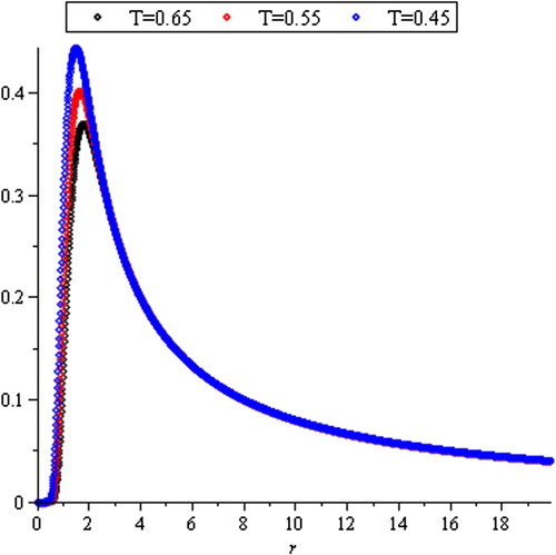
Figure 3 represents the Wiener process range density function after deleting a few stochastic volatility interval $[1,3]$ with increasing the value of $T$.

Figure 3. Probability density function of R(T).

It is clear that the probability of the truncated area is equally distributed between the remaining parts and make the probability of some values of R(T) attain its maximum value (approximately 0.73). On the contrary, the maximum probability of some values of R(T) is approximately 0.43 (see Figure 1). But the two curves confine two equal areas. From here, we can delete the few stochastic volatility interval from the domain of the Wiener process range by using the probability density function (4).

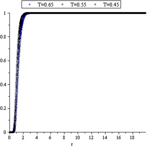
The cumulative distribution function of (4) is given by $G_{R\left(T\right)}\left(r\right)=\left\{\begin{array}{ll}{\int }_0^r{g}_{R\left(T\right)}\left(r\right)\text{d}r,& 0<r<\alpha ,\\ {\int }_0^r{g}_{R\left(T\right)}\left(r\right)\text{d}r+{\int }_{\alpha }^{\beta }{g}_{R\left(T\right)}\left(r\right)& \\ \text{d}r+{\int }_{\beta }^r{g}_{R\left(T\right)}\left(r\right)\text{d}r,& \beta <r<\mathrm{\infty }.\end{array}\right.$

Since the time interval which not containing any random fluctuations was deleted, the probability of this interval should be distributed on the other parts. Consequently, we have

(5) $\begin{array}{rl}& \\ G_{R\left(T\right)}\left(r\right)& =\left\{\begin{array}{ll}{\int }_0^r{g}_{R\left(T\right)}\left(r\right)\text{d}r,& 0<r<\alpha ,\\ {\int }_0^{\alpha }{g}_{R\left(T\right)}\left(r\right)dr+{\int }_{\beta }^r{g}_{R\left(T\right)}\left(r\right)\text{d}r,& \beta <r<\mathrm{\infty },\end{array}\right.\\ & =\left\{\begin{array}{l}\frac{\sum _{k=1}^{\mathrm{\infty }}\left(\frac{8}{{(2k-1)}^2{\pi }^2}+\frac{8T}{r^2}\right)\exp \left[-\frac{{(2k-1)}^2{\pi }^{2}T}{2r^2}\right]}{1-\sum _{k=1}^{\mathrm{\infty }}\left(\frac{8}{{(2k-1)}^2{\pi }^2}+\frac{8T}{{\beta }^2}\right)\exp \left[-\frac{{(2k-1)}^2{\pi }^{2}T}{2{\beta }^2}\right]+\sum _{k=1}^{\mathrm{\infty }}\left(\frac{8}{{(2k-1)}^2{\pi }^2}+\frac{8T}{{\alpha }^2}\right)\exp \left[-\frac{{(2k-1)}^2{\pi }^{2}T}{2{\alpha }^2}\right]},\\ \\ 0<r<\alpha ,\\ \frac{\sum _{k=1}^{\mathrm{\infty }}\left(\frac{8}{{(2k-1)}^2{\pi }^2}+\frac{8T}{{\alpha }^2}\right)\exp \left[-\frac{{(2k-1)}^2{\pi }^{2}T}{2{\alpha }^2}\right]}{1-\sum _{k=1}^{\mathrm{\infty }}\left(\frac{8}{{(2k-1)}^2{\pi }^2}+\frac{8T}{{\beta }^2}\right)\exp \left[-\frac{{(2k-1)}^2{\pi }^{2}T}{2{\beta }^2}\right]+\sum _{k=1}^{\mathrm{\infty }}\left(\frac{8}{{(2k-1)}^2{\pi }^2}+\frac{8T}{{\alpha }^2}\right)\exp \left[-\frac{{(2k-1)}^2{\pi }^{2}T}{2{\alpha }^2}\right]}+\\ \frac{\sum _{k=1}^{\mathrm{\infty }}\left(\frac{8}{{(2k-1)}^2{\pi }^2}+\frac{8T}{r^2}\right)\exp \left[-\frac{{(2k-1)}^2{\pi }^{2}T}{2r^2}\right]-\sum _{k=1}^{\mathrm{\infty }}\left(\frac{8}{{(2k-1)}^2{\pi }^2}+\frac{8T}{{\beta }^2}\right)\exp \left[-\frac{{(2k-1)}^2{\pi }^{2}T}{2{\beta }^2}\right]}{1-\sum _{k=1}^{\mathrm{\infty }}\left(\frac{8}{{(2k-1)}^2{\pi }^2}+\frac{8T}{{\beta }^2}\right)\exp \left[-\frac{{(2k-1)}^2{\pi }^{2}T}{2{\beta }^2}\right]+\sum _{k=1}^{\mathrm{\infty }}\left(\frac{8}{{(2k-1)}^2{\pi }^2}+\frac{8T}{{\alpha }^2}\right)\exp \left[-\frac{{(2k-1)}^2{\pi }^{2}T}{2{\alpha }^2}\right]},\\ \\ \beta <r<\mathrm{\infty },\end{array}\right.\end{array}$(5)

and it is represented in Figure 4.

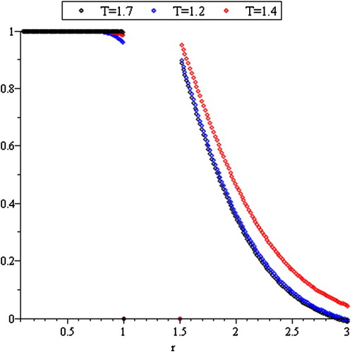
Figure 4. Cumulative distribution function of $R\left(T\right)$.

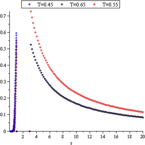
We know that the survival function is given by ${\overline{G}}_{R\left(T\right)}(.)=1-G_{R\left(T\right)}\left(r\right)$, but according to Definition 2.1, the internal truncated survival function of $R\left(T\right)$ is given by

(6) $\begin{array}{rl}{\overline{G}}_{R\left(T\right)}\left(r\right)& =\left\{\begin{array}{ll}1-{\int }_0^r{g}_{R\left(T\right)}\left(r\right)\text{d}r,& 0<r<\alpha ,\\ \left(1-{\int }_0^{\alpha }{g}_{R\left(T\right)}\left(r\right)\text{d}r\right)& \\ -\left({\int }_0^{\alpha }{g}_{R\left(T\right)}\left(r\right)\text{d}r+{\int }_{\beta }^r{g}_{R\left(T\right)}\left(r\right)\text{d}r\right),\\ & \beta <r<\mathrm{\infty },\end{array}\right.\\ & =\left\{\begin{array}{ll}1-{\int }_0^r{g}_{R\left(T\right)}\left(r\right)\text{d}r,& 0<r<\alpha ,\\ 1-2{\int }_0^{\alpha }{g}_{R\left(T\right)}\left(r\right)\text{d}r-{\int }_{\beta }^r{g}_{R\left(T\right)}\left(r\right)\text{d}r,& \beta <r<\mathrm{\infty },\end{array}\right.\\ & =\left\{\begin{array}{l}1-\frac{\sum _{k=1}^{\mathrm{\infty }}\left(\frac{8}{{(2k-1)}^2{\pi }^2}+\frac{8T}{r^2}\right)\exp \left[-\frac{{(2k-1)}^2{\pi }^{2}T}{2r^2}\right]}{1-\sum _{k=1}^{\mathrm{\infty }}\left(\frac{8}{{(2k-1)}^2{\pi }^2}+\frac{8T}{{\beta }^2}\right)\exp \left[-\frac{{(2k-1)}^2{\pi }^{2}T}{2{\beta }^2}\right]+\sum _{k=1}^{\mathrm{\infty }}\left(\frac{8}{{(2k-1)}^2{\pi }^2}+\frac{8T}{{\alpha }^2}\right)\exp \left[-\frac{{(2k-1)}^2{\pi }^{2}T}{2{\alpha }^2}\right]},\\ 0<r<\alpha ,\\ 1-\frac{2\sum _{k=1}^{\mathrm{\infty }}\left(\frac{8}{{(2k-1)}^2{\pi }^2}+\frac{8T}{{\alpha }^2}\right)\exp \left[-\frac{{(2k-1)}^2{\pi }^{2}T}{2{\alpha }^2}\right]}{1-\sum _{k=1}^{\mathrm{\infty }}\left(\frac{8}{{(2k-1)}^2{\pi }^2}+\frac{8T}{{\beta }^2}\right)\exp \left[-\frac{{(2k-1)}^2{\pi }^{2}T}{2{\beta }^2}\right]+\sum _{k=1}^{\mathrm{\infty }}\left(\frac{8}{{(2k-1)}^2{\pi }^2}+\frac{8T}{{\alpha }^2}\right)\exp \left[-\frac{{(2k-1)}^2{\pi }^{2}T}{2{\alpha }^2}\right]}\\ -\frac{\sum _{k=1}^{\mathrm{\infty }}\left(\frac{8}{{(2k-1)}^2{\pi }^2}+\frac{8T}{r^2}\right)\exp \left[-\frac{{(2k-1)}^2{\pi }^{2}T}{2r^2}\right]-\sum _{k=1}^{\mathrm{\infty }}\left(\frac{8}{{(2k-1)}^2{\pi }^2}+\frac{8T}{{\beta }^2}\right)\exp \left[-\frac{{(2k-1)}^2{\pi }^{2}T}{2{\beta }^2}\right]}{1-\sum _{k=1}^{\mathrm{\infty }}\left(\frac{8}{{(2k-1)}^2{\pi }^2}+\frac{8T}{{\beta }^2}\right)\exp \left[-\frac{{(2k-1)}^2{\pi }^{2}T}{2{\beta }^2}\right]+\sum _{k=1}^{\mathrm{\infty }}\left(\frac{8}{{(2k-1)}^2{\pi }^2}+\frac{8T}{{\alpha }^2}\right)\exp \left[-\frac{{(2k-1)}^2{\pi }^{2}T}{2{\alpha }^2}\right]},\\ \beta <r<\mathrm{\infty },\end{array}\right.\end{array}$(6)

From Figure 5, we notice that the internal truncated survival function is decreasing by increasing the value of $T.$

Figure 5. Survival function of R(T).

3. Some statistical properties

Teamah et al. [3] studied various statistical properties of the stock price distributions that arise when prices follow a Wiener process range distribution (truncated and nontruncated). Rather than presenting the shape of the probability distribution and the hazard rate functions, a comprehensive treatment of the statistical properties of this distribution is presented including, moments, Bonferroni curve, stress-strength parameter, Lorenz curve and Gini's index.

3.1. Reliability properties

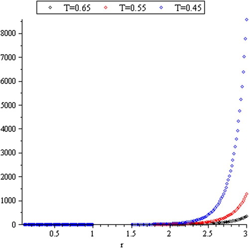
In some cases, the stock price may be changed to a large extent, over a day or a month or a year. This differs continuous movement which known as the price fluctuations, where the price of the stock price is more volatile than other stock price. Thus, the swings between fall and rise of the stock price during the time interval $(0,T)$ affect the risk rate (hazard rate). The hazard function is a very useful function in lifetime analysis, see Marshall and Olkin [12]. Generally, Teamah et al. [3] studied this effect when the range is bounded. In the case of deleting a few stochastic volatility interval from the range, the hazard rate function is given by

(7) $\begin{array}{rl}{z}_{R\left(T\right)}\left(r\right)& =\left\{\begin{array}{ll}\frac{g_{R\left(T\right)}\left(r\right)}{1-G_{R\left(t\right)}\left(r\right)},& 0<r<\alpha ,\\ \frac{g_{R\left(T\right)}\left(r\right)}{1-2G_{R\left(t\right)}\left(\alpha \right)-G_{R\left(t\right)}\left(r\right)},& \beta <r<\mathrm{\infty },\end{array}\right.\\ & =\left\{\begin{array}{ll}\frac{\frac{{\left(\frac{2}{\pi }\right)}^{\frac{1}{2}}{r}^{-1}{\left(2\pi \right)}^{\frac{1}{2}}{\left(\frac{r{T}^{-\frac{1}{2}}}{2}\right)}^{-1}\sum _{k=1}^{\mathrm{\infty }}\exp \left[-\frac{{(2k-1)}^2{\pi }^2}{8}.{\left(\frac{r{T}^{-\frac{1}{2}}}{2}\right)}^{-2}\right]}{1-\sum _{k=1}^{\mathrm{\infty }}\left(\frac{8}{{(2k-1)}^2{\pi }^2}+\frac{8T}{{\beta }^2}\right)\exp \left[-\frac{{(2k-1)}^2{\pi }^{2}T}{2{\beta }^2}\right]+\sum _{k=1}^{\mathrm{\infty }}\left(\frac{8}{{(2k-1)}^2{\pi }^2}+\frac{8T}{{\alpha }^2}\right)\exp \left[-\frac{{(2k-1)}^2{\pi }^{2}T}{2{\alpha }^2}\right]}}{1-\left(\frac{\sum _{k=1}^{\mathrm{\infty }}\left(\frac{8}{{(2k-1)}^2{\pi }^2}+\frac{8T}{r^2}\right)\exp \left[-\frac{{(2k-1)}^2{\pi }^{2}T}{2r^2}\right]}{1-\sum _{k=1}^{\mathrm{\infty }}\left(\frac{8}{{(2k-1)}^2{\pi }^2}+\frac{8T}{{\beta }^2}\right)\exp \left[-\frac{{(2k-1)}^2{\pi }^{2}T}{2{\beta }^2}\right]+\sum _{k=1}^{\mathrm{\infty }}\left(\frac{8}{{(2k-1)}^2{\pi }^2}+\frac{8T}{{\alpha }^2}\right)\exp \left[-\frac{{(2k-1)}^2{\pi }^{2}T}{2{\alpha }^2}\right]}\right)},& 0<r<\alpha \\ \frac{\frac{{\left(\frac{2}{\pi }\right)}^{\frac{1}{2}}{r}^{-1}{\left(2\pi \right)}^{\frac{1}{2}}{\left(\frac{r{T}^{-\frac{1}{2}}}{2}\right)}^{-1}\sum _{k=1}^{\mathrm{\infty }}\exp \left[-\frac{{(2k-1)}^2{\pi }^2}{8}.{\left(\frac{r{T}^{-\frac{1}{2}}}{2}\right)}^{-2}\right]}{1-\sum _{k=1}^{\mathrm{\infty }}\left(\frac{8}{{(2k-1)}^2{\pi }^2}+\frac{8T}{{\beta }^2}\right)\exp \left[-\frac{{(2k-1)}^2{\pi }^{2}T}{2{\beta }^2}\right]+\sum _{k=1}^{\mathrm{\infty }}\left(\frac{8}{{(2k-1)}^2{\pi }^2}+\frac{8T}{{\alpha }^2}\right)\exp \left[-\frac{{(2k-1)}^2{\pi }^{2}T}{2{\alpha }^2}\right]}}{\begin{array}{l}\left[1-\left(\frac{\sum _{k=1}^{\mathrm{\infty }}\left(\frac{8}{{(2k-1)}^2{\pi }^2}+\frac{8T}{{\alpha }^2}\right)\exp \left[-\frac{{(2k-1)}^2{\pi }^{2}T}{2{\alpha }^2}\right]}{1-\sum _{k=1}^{\mathrm{\infty }}\left(\frac{8}{{(2k-1)}^2{\pi }^2}+\frac{8T}{{\beta }^2}\right)\exp \left[-\frac{{(2k-1)}^2{\pi }^{2}T}{2{\beta }^2}\right]+\sum _{k=1}^{\mathrm{\infty }}\left(\frac{8}{{(2k-1)}^2{\pi }^2}+\frac{8T}{{\alpha }^2}\right)\exp \left[-\frac{{(2k-1)}^2{\pi }^{2}T}{2{\alpha }^2}\right]}\right)\right.\\ \left.\begin{array}{c}\end{array}-\left(\frac{\sum _{k=1}^{\mathrm{\infty }}\left(\frac{8}{{(2k-1)}^2{\pi }^2}+\frac{8T}{r^2}\right)\exp \left[-\frac{{(2k-1)}^2{\pi }^{2}T}{2r^2}\right]-\sum _{k=1}^{\mathrm{\infty }}\left(\frac{8}{{(2k-1)}^2{\pi }^2}+\frac{8T}{{\beta }^2}\right)\exp \left[-\frac{{(2k-1)}^2{\pi }^{2}T}{2{\beta }^2}\right]}{1-\sum _{k=1}^{\mathrm{\infty }}\left(\frac{8}{{(2k-1)}^2{\pi }^2}+\frac{8T}{{\beta }^2}\right)\exp \left[-\frac{{(2k-1)}^2{\pi }^{2}T}{2{\beta }^2}\right]+\sum _{k=1}^{\mathrm{\infty }}\left(\frac{8}{{(2k-1)}^2{\pi }^2}+\frac{8T}{{\alpha }^2}\right)\exp \left[-\frac{{(2k-1)}^2{\pi }^{2}T}{2{\alpha }^2}\right]}\right)\right],\end{array}}& \beta <r<\mathrm{\infty },\end{array}\right.\end{array}$(7)

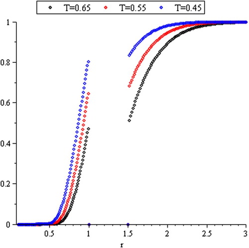
and it is represented in Figure 6.

Figure 6. Hazard rate function of R(T).

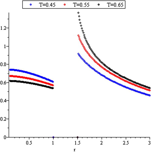
Also, the reversed hazard rate function is

(8) $\begin{array}{rl}{\tilde{z}}_{R\left(T\right)}\left(r\right)& =\left\{\begin{array}{ll}\frac{g_{R\left(T\right)}\left(r\right)}{G_{R\left(t\right)}\left(r\right)},& 0<r<\alpha ,\\ \frac{g_{R\left(T\right)}\left(r\right)}{G_{R\left(t\right)}\left(\alpha \right)+G_{R\left(t\right)}\left(r\right)},& \beta <r<\mathrm{\infty },\end{array}\right.\\ & =\left\{\begin{array}{ll}\frac{\frac{{\left(\frac{2}{\pi }\right)}^{\frac{1}{2}}{r}^{-1}{\left(2\pi \right)}^{\frac{1}{2}}{\left(\frac{r{T}^{-\frac{1}{2}}}{2}\right)}^{-1}\sum _{k=1}^{\mathrm{\infty }}\exp \left[-\frac{{(2k-1)}^2{\pi }^2}{8}.{\left(\frac{r{T}^{-\frac{1}{2}}}{2}\right)}^{-2}\right]}{1-\sum _{k=1}^{\mathrm{\infty }}\left(\frac{8}{{(2k-1)}^2{\pi }^2}+\frac{8T}{{\beta }^2}\right)\exp \left[-\frac{{(2k-1)}^2{\pi }^{2}T}{2{\beta }^2}\right]+\sum _{k=1}^{\mathrm{\infty }}\left(\frac{8}{{(2k-1)}^2{\pi }^2}+\frac{8T}{{\alpha }^2}\right)\exp \left[-\frac{{(2k-1)}^2{\pi }^{2}T}{2{\alpha }^2}\right]}}{\frac{\sum _{k=1}^{\mathrm{\infty }}\left(\frac{8}{{(2k-1)}^2{\pi }^2}+\frac{8T}{r^2}\right)\exp \left[-\frac{{(2k-1)}^2{\pi }^{2}T}{2r^2}\right]}{1-\sum _{k=1}^{\mathrm{\infty }}\left(\frac{8}{{(2k-1)}^2{\pi }^2}+\frac{8T}{{\beta }^2}\right)\exp \left[-\frac{{(2k-1)}^2{\pi }^{2}T}{2{\beta }^2}\right]+\sum _{k=1}^{\mathrm{\infty }}\left(\frac{8}{{(2k-1)}^2{\pi }^2}+\frac{8T}{{\alpha }^2}\right)\exp \left[-\frac{{(2k-1)}^2{\pi }^{2}T}{2{\alpha }^2}\right]},}& 0<r<\alpha ,\\ \frac{\frac{{\left(\frac{2}{\pi }\right)}^{\frac{1}{2}}{r}^{-1}{\left(2\pi \right)}^{\frac{1}{2}}{\left(\frac{r{T}^{-\frac{1}{2}}}{2}\right)}^{-1}\sum _{k=1}^{\mathrm{\infty }}\exp \left[-\frac{{(2k-1)}^2{\pi }^2}{8}.{\left(\frac{r{T}^{-\frac{1}{2}}}{2}\right)}^{-2}\right]}{1-\sum _{k=1}^{\mathrm{\infty }}\left(\frac{8}{{(2k-1)}^2{\pi }^2}+\frac{8T}{{\beta }^2}\right)\exp \left[-\frac{{(2k-1)}^2{\pi }^{2}T}{2{\beta }^2}\right]+\sum _{k=1}^{\mathrm{\infty }}\left(\frac{8}{{(2k-1)}^2{\pi }^2}+\frac{8T}{{\alpha }^2}\right)\exp \left[-\frac{{(2k-1)}^2{\pi }^{2}T}{2{\alpha }^2}\right]}}{\begin{array}{l}\left[\left(\frac{\sum _{k=1}^{\mathrm{\infty }}\left(\frac{8}{{(2k-1)}^2{\pi }^2}+\frac{8T}{{\alpha }^2}\right)\exp \left[-\frac{{(2k-1)}^2{\pi }^{2}T}{2{\alpha }^2}\right]}{1-\sum _{k=1}^{\mathrm{\infty }}\left(\frac{8}{{(2k-1)}^2{\pi }^2}+\frac{8T}{{\beta }^2}\right)\exp \left[-\frac{{(2k-1)}^2{\pi }^{2}T}{2{\beta }^2}\right]+\sum _{k=1}^{\mathrm{\infty }}\left(\frac{8}{{(2k-1)}^2{\pi }^2}+\frac{8T}{{\alpha }^2}\right)\exp \left[-\frac{{(2k-1)}^2{\pi }^{2}T}{2{\alpha }^2}\right]}\right)\right.\\ \left.\begin{array}{c}\end{array}+\frac{\sum _{k=1}^{\mathrm{\infty }}\left(\frac{8}{{(2k-1)}^2{\pi }^2}+\frac{8T}{r^2}\right)\exp \left[-\frac{{(2k-1)}^2{\pi }^{2}T}{2r^2}\right]-\sum _{k=1}^{\mathrm{\infty }}\left(\frac{8}{{(2k-1)}^2{\pi }^2}+\frac{8T}{{\beta }^2}\right)\exp \left[-\frac{{(2k-1)}^2{\pi }^{2}T}{2{\beta }^2}\right]}{1-\sum _{k=1}^{\mathrm{\infty }}\left(\frac{8}{{(2k-1)}^2{\pi }^2}+\frac{8T}{{\beta }^2}\right)\exp \left[-\frac{{(2k-1)}^2{\pi }^{2}T}{2{\beta }^2}\right]+\sum _{k=1}^{\mathrm{\infty }}\left(\frac{8}{{(2k-1)}^2{\pi }^2}+\frac{8T}{{\alpha }^2}\right)\exp \left[-\frac{{(2k-1)}^2{\pi }^{2}T}{2{\alpha }^2}\right]}\right],\end{array}}& \beta <r<\mathrm{\infty }.\end{array}\right.\end{array}$(8)

Clearly, when the range $R\left(T\right)$ increases, the hazard rate approaches zero and increases rapidly as $R\left(T\right)$ falls to zero (see Figure 7).

Figure 7. Reversed hazard rate function of R(T).

3.2. Moments

Moments are useful for the internal truncated distribution of the Wiener range. The generating, characteristic functions and moments of the range distribution (1) [2] are found. Also, Teamah et al. [3] presented some statistical properties of the double truncated Wiener range distribution including moments. Here, if $R\left(T\right)$ has one internal truncation and $r>0,$ $T>0$ then the moment generating function (m.g.f.) of $R\left(T\right)$ takes the form

(9) $\begin{array}{rl}M\left(t\right)=E\left(e^{tr}\right)& =\underset{\upsilon \to 0}{lim}{\int }_{\upsilon }^{\alpha }\frac{e^{tr}{\left(\frac{2}{\pi }\right)}^{\frac{1}{2}}{r}^{-1}{\left(2\pi \right)}^{\frac{1}{2}}{\left(\frac{r{T}^{-\frac{1}{2}}}{2}\right)}^{-1}\sum _{k=1}^{\mathrm{\infty }}\exp \left[-\frac{{(2k-1)}^2{\pi }^2}{8}.{\left(\frac{r{T}^{-\frac{1}{2}}}{2}\right)}^{-2}\right]}{1-\sum _{k=1}^{\mathrm{\infty }}\left(\frac{8}{{(2k-1)}^2{\pi }^2}+\frac{8T}{{\beta }^2}\right)\exp \left[-\frac{{(2k-1)}^2{\pi }^{2}T}{2{\beta }^2}\right]+\sum _{k=1}^{\mathrm{\infty }}\left(\frac{8}{{(2k-1)}^2{\pi }^2}+\frac{8T}{{\alpha }^2}\right)\exp \left[-\frac{{(2k-1)}^2{\pi }^{2}T}{2{\alpha }^2}\right]}\text{d}r\\ & +\underset{\hslash \to \mathrm{\infty }}{lim}{\int }_{\beta }^{\hslash }\frac{e^{tr}{\left(\frac{2}{\pi }\right)}^{\frac{1}{2}}{r}^{-1}{\left(2\pi \right)}^{\frac{1}{2}}{\left(\frac{r{T}^{-\frac{1}{2}}}{2}\right)}^{-1}\sum _{k=1}^{\mathrm{\infty }}\exp \left[-\frac{{(2k-1)}^2{\pi }^2}{8}.{\left(\frac{r{T}^{-\frac{1}{2}}}{2}\right)}^{-2}\right]}{1-\sum _{k=1}^{\mathrm{\infty }}\left(\frac{8}{{(2k-1)}^2{\pi }^2}+\frac{8T}{{\beta }^2}\right)\exp \left[-\frac{{(2k-1)}^2{\pi }^{2}T}{2{\beta }^2}\right]+\sum _{k=1}^{\mathrm{\infty }}\left(\frac{8}{{(2k-1)}^2{\pi }^2}+\frac{8T}{{\alpha }^2}\right)\exp \left[-\frac{{(2k-1)}^2{\pi }^{2}T}{2{\alpha }^2}\right]}\text{d}r,\end{array}$(9)

where $\upsilon \to 0$ and not equal to 0, because when displaying stock for sale (at the moment 0) the difference between the highest and the lowest prices is greater than zero, even by a small percentage $\upsilon$. At this moment, there is only the highest price either the lower price equal to 0.

Assuming that $\upsilon =a,\alpha =b$, $\begin{array}{rl}& I(\upsilon ,\alpha ,t,T)={\int }_{\upsilon }^{\alpha }{e}^{tr}{\left(\frac{2}{\pi }\right)}^{\frac{1}{2}}{r}^{-1}{\left(2\pi \right)}^{\frac{1}{2}}{\left(\frac{r{T}^{-\frac{1}{2}}}{2}\right)}^{-1}\\ & \times \sum _{k=1}^{\mathrm{\infty }}\exp \left[-\frac{{(2k-1)}^2{\pi }^2}{8}.{\left(\frac{r{T}^{-\frac{1}{2}}}{2}\right)}^{-2}\right]\text{d}r,\end{array}$ and $\begin{array}{rl}& J(\beta ,t,T)={\int }_{\beta }^{\mathrm{\infty }}{e}^{tr}{\left(\frac{2}{\pi }\right)}^{\frac{1}{2}}{r}^{-1}{\left(2\pi \right)}^{\frac{1}{2}}{\left(\frac{r{T}^{-\frac{1}{2}}}{2}\right)}^{-1}\\ & \times \sum _{k=1}^{\mathrm{\infty }}\exp \left[-\frac{{(2k-1)}^2{\pi }^2}{8}.{\left(\frac{r{T}^{-\frac{1}{2}}}{2}\right)}^{-2}\right]\text{d}r.\end{array}$ Thus, one can get (10) $I(a,b,t,T)={\int }_a^b\sum _{k=1}^{\mathrm{\infty }}\left({\alpha }_k+\frac{\hat{a}}{r^2}\right)e^{\left(tr-\frac{{\beta }_k}{r^2}\right)}\text{d}r.$(10)

And ${\alpha }_k=\frac{8}{{(2k-1)}^2{\pi }^2},\hat{a}=8T,{\beta }_k=\frac{{(2k-1)}^2{\pi }^{2}T}{2}.$ It is known that the expansion of the exponential function is valid for $r\in (-\mathrm{\infty },\mathrm{\infty })$ and gives a uniformly convergent series, then we get $\begin{array}{rl}{e}^{\left(tr-\frac{{\beta }_k}{r^2}\right)}& =\sum _{m=0}^{\mathrm{\infty }}\frac{{e^{\left(tr-\frac{{\beta }_k}{r^2}\right)}}^m}{m!}=1+tr-\frac{{\beta }_k}{r^2}+\sum _{m=2}^{\mathrm{\infty }}\frac{{e^{\left(tr-\frac{{\beta }_k}{r^2}\right)}}^m}{m!}\\ & =1+tr-\frac{{\beta }_k}{r^2}+\sum _{m=2}^{\mathrm{\infty }}\sum _{\mu =0}^m\frac{t^{m-\mu }}{m!}\left(\begin{array}{l}m\\ \mu \end{array}\right)(-{\beta }_k{)}^{\mu }{r}^{m-3\mu }.\end{array}$Let $I(a,b,t,T)=I_1(a,b,t,T)+I_2(a,b,t,T)$, where (11) $\begin{array}{rl}{I}_1(a,b,t,T)& =\sum _{k=1}^{\mathrm{\infty }}{\int }_a^b{\alpha }_k{e}^{\left(tr-\frac{{\beta }_k}{r^2}\right)}\text{d}r=\sum _{k=1}^{\mathrm{\infty }}{\int }_a^b{\alpha }_k\left(1+tr-\frac{{\beta }_k}{r^2}\right.\\ & \left.+\sum _{m=2}^{\mathrm{\infty }}\sum _{\mu =0}^m\frac{t^{m-\mu }}{m!}\left(\begin{array}{l}m\\ \mu \end{array}\right){(-{\beta }_k)}^{\mu }{r}^{m-3\mu }\right)\text{d}r,\end{array}$(11) and (12) $\begin{array}{rl}& I_2(a,b,t,T)=\sum _{k=1}^{\mathrm{\infty }}{\int }_a^b\frac{\hat{a}}{r^2}{e}^{\left(tr-\frac{{\beta }_k}{r^2}\right)}\text{d}r=\hat{a}\sum _{k=1}^{\mathrm{\infty }}{\int }_a^b{r}^{-2}\\ & +t{r}^{-1}-\frac{{\beta }_k}{r^2}+\sum _{m=2}^{\mathrm{\infty }}\sum _{\mu =0}^m\frac{t^{m-\mu }}{m!}\left(\begin{array}{l}m\\ \mu \end{array}\right){(-{\beta }_k)}^{\mu }{r}^{m-2-3\mu }\text{d}r.\end{array}$(12) By solving the following equations, (13) $m-3\mu =-1,$(13) (14) $m-2-3\mu =-1,$(14) as diophantine equations, we have the set solution for (13) given by (15) $S_1=(m_{S_1},{\mu }_{S_1})=\left\{\right(2,1),(5,2),(8,3),(11,4),\dots \},$(15) and for (14) (16) $S_2=(m_{S_2},{\mu }_{S_2})=\left\{\right(4,1),(7,2),(10,3),(13,4),\dots \}.$(16)

Hence, $I_1(a,b,t,T)$ can be written as follows: (17) $\begin{array}{rl}& I_1(a,b,t,T)\\ & =\sum _{k=1}^{\mathrm{\infty }}{\alpha }_k\left[(b-a)+\frac{t}{2}(b^2-a^2)-{\beta }_k\left(\frac{1}{a}-\frac{1}{b}\right)\right]\\ & +\sum _{k=1}^{\mathrm{\infty }}{\alpha }_k\stackrel{\mathrm{\forall }m,(\mu \ne {\mu }_{S_1}\wedge m=m_{S_1})}{\overbrace{\left[\begin{array}{c}\sum _{m=2}^{\mathrm{\infty }}\sum _{\mu =0}^m\left(\begin{array}{l}m\\ \mu \end{array}\right)\frac{{(-{\beta }_k)}^{\mu }{t}^{m-\mu }}{m!(m+1-3\mu )}\\ \left(b^{m+1-3\mu }-a^{m+1-3\mu }\right)\end{array}\right]}}\\ & +\sum _{k=1}^{\mathrm{\infty }}{\alpha }_k\left(\sum _{(m,\mu )\in S_1}\left(\begin{array}{l}m\\ \mu \end{array}\right)\frac{{(-{\beta }_k)}^{\mu }}{m!}{t}^{m-\mu }\ln \frac{b}{a}\right),\end{array}$(17)

Also, $I_2(a,b,t,T)$ can be written as follows: (18) $\begin{array}{rl}& I_2(a,b,t,T)\\ & =\hat{a}\sum _{k=1}^{\mathrm{\infty }}\left[(a^{-1}-b^{-1})+t\ln \frac{b}{a}-\frac{{\beta }_k}{3}\left(\frac{1}{a^3}-\frac{1}{b^3}\right)\right]\\ & +\hat{a}\sum _{k=1}^{\mathrm{\infty }}\stackrel{\mathrm{\forall }m,(\mu \ne {\mu }_{S_2}\wedge m=m_{S_2})}{\overbrace{\left[\begin{array}{c}\sum _{m=2}^{\mathrm{\infty }}\sum _{\mu =0}^m\left(\begin{array}{l}m\\ \mu \end{array}\right)\frac{{(-{\beta }_k)}^{\mu }{t}^{m-\mu }}{m!(m-1-3\mu )}\\ \left(b^{m-1-3\mu }-a^{m-1-3\mu }\right)\end{array}\right]}}\\ & +\hat{a}\sum _{k=1}^{\mathrm{\infty }}\left(\sum _{(m,\mu )\in S_2}\left(\begin{array}{l}m\\ \mu \end{array}\right)\frac{{(-{\beta }_k)}^{\mu }}{m!}{t}^{m-\mu }\ln \frac{b}{a}\right).\end{array}$(18)

In real-life problem and at any time, we do not have the ability to see that the difference between the highest and the lowest prices tends to infinity. Infinity here means that the difference attains its maximum which the statistician and the economists consider them as a known value. Thus, in mathematical calculations we can consider that the greatest and the maximum value of the difference is equal to $\hslash$ which tends to infinity (i.e. $\hslash \to \mathrm{\infty }$).

Now, the integral $J(\beta ,t,T)$ is equivalent to the integral $J(\beta ,\hslash ,t,T)$ which can be calculated as (10). Compensation for $\upsilon =\beta ,\alpha =\hslash$ in (17) and (18) we have, $J(\beta ,t,T)$=$I_1(\beta ,\hslash ,t,T)+I_2(\beta ,\hslash ,t,T)$

(19) $\begin{array}{rl}& =\sum _{k=1}^{\mathrm{\infty }}{\alpha }_k\left[(\hslash -\beta )+\frac{t}{2}({\hslash }^2-{\beta }^2)-{\beta }_k\left(\frac{1}{\beta }-\frac{1}{\hslash }\right)\right]+\sum _{k=1}^{\mathrm{\infty }}{\alpha }_k\stackrel{\mathrm{\forall }m,(\mu \ne {\mu }_{S_1}\wedge m=m_{S_1})}{\overbrace{\left[\sum _{m=2}^{\mathrm{\infty }}\sum _{\mu =0}^m\left(\begin{array}{l}m\\ \mu \end{array}\right)\frac{{(-{\beta }_k)}^{\mu }{t}^{m-\mu }}{m!(m+1-3\mu )}\left({\hslash }^{m+1-3\mu }-{\beta }^{m+1-3\mu }\right)\right]}}\\ & +\sum _{k=1}^{\mathrm{\infty }}{\alpha }_k\left(\sum _{(m,\mu )\in S_1}\left(\begin{array}{l}m\\ \mu \end{array}\right)\frac{{(-{\beta }_k)}^{\mu }}{m!}{t}^{m-\mu }\ln \frac{\hslash }{\beta }\right)+\hat{a}\sum _{k=1}^{\mathrm{\infty }}\left[({\beta }^{-1}-{\hslash }^{-1})+t\ln \frac{\hslash }{\beta }-\frac{{\beta }_k}{3}\left(\frac{1}{{\beta }^3}-\frac{1}{{\hslash }^3}\right)\right]\\ & +\hat{a}\sum _{k=1}^{\mathrm{\infty }}\stackrel{\mathrm{\forall }m,(\mu \ne {\mu }_{S_2}\wedge m=m_{S_2})}{\overbrace{\left[\sum _{m=2}^{\mathrm{\infty }}\sum _{\mu =0}^m\left(\begin{array}{l}m\\ \mu \end{array}\right)\frac{{(-{\beta }_k)}^{\mu }{t}^{m-\mu }}{m!(m-1-3\mu )}\left({\hslash }^{m-1-3\mu }-{\beta }^{m-1-3\mu }\right)\right]}}+\hat{a}\sum _{k=1}^{\mathrm{\infty }}\left(\sum _{(m,\mu )\in S_2}\left(\begin{array}{l}m\\ \mu \end{array}\right)\frac{{(-{\beta }_k)}^{\mu }}{m!}{t}^{m-\mu }\ln \frac{\hslash }{\beta }\right).\end{array}$(19)

Consequently, from (17), (18) and (19) we have,

(20) $M\left(t\right)=E\left(e^{tr}\right)=\frac{\left|\frac{T^{\frac{-1}{2}}}{2}\right|\left(\underset{\upsilon \to 0}{lim}\left[I_1(\upsilon ,\alpha ,t,T)+I_2(\upsilon ,\alpha ,t,T)\right]+\underset{\hslash \to \mathrm{\infty }}{lim}J(\beta ,\hslash ,t,T)\right)}{1-\sum _{k=1}^{\mathrm{\infty }}\left(\frac{8}{{(2k-1)}^2{\pi }^2}+\frac{8T}{{\beta }^2}\right)\exp \left[-\frac{{(2k-1)}^2{\pi }^{2}T}{2{\beta }^2}\right]+\sum _{k=1}^{\mathrm{\infty }}\left(\frac{8}{{(2k-1)}^2{\pi }^2}+\frac{8T}{{\alpha }^2}\right)\exp \left[-\frac{{(2k-1)}^2{\pi }^{2}T}{2{\alpha }^2}\right]}.$(20)

According to the solution method by Teamah et al. [3] and using (4), one can obtain the moments of $R\left(T\right)$ about the origin by

(21a) $\begin{array}{rl}E\left(r^q\right)& ={\int }_{\upsilon }^{\alpha }{r}^q{g}_{R\left(T\right)}\left(r\right)\text{d}r+{\int }_{\beta }^{\hslash }{g}_{R\left(T\right)}\left(r\right)\text{d}r\\ & =\frac{2^q{T}^{\frac{q}{2}}\sum _{k=1}^{\mathrm{\infty }}\left({\upsilon }^{-2+q}\xi \left[\frac{q}{2},\frac{{\left(2k-1\right)}^2{\pi }^2}{8{\upsilon }^2}\right]-{\alpha }^{-2+q}\xi \left[\frac{q}{2},\frac{{\left(2k-1\right)}^2{\pi }^2}{8{\alpha }^2}\right]+{\text{ƛ}}_k\right)}{\sum _{k=1}^{\mathrm{\infty }}\left(\frac{8}{{(2k-1)}^2{\pi }^2}+8T{\alpha }^{-2}\right)e^{-\frac{{(2k-1)}^2{\pi }^{2}T{\alpha }^{-2}}{2}}-\sum _{k=1}^{\mathrm{\infty }}\left(\frac{8}{{(2k-1)}^2{\pi }^2}+8T{\upsilon }^{-2}\right)e^{-\frac{{(2k-1)}^2{\pi }^{2}T{\upsilon }^{-2}}{2}}}\\ & +\frac{2^q{T}^{\frac{q}{2}}\sum _{k=1}^{\mathrm{\infty }}\left({\beta }^{-2+q}\xi \left[\frac{q}{2},\frac{{\left(2k-1\right)}^2{\pi }^2}{8{\beta }^2}\right]-{\hslash }^{-2+q}\xi \left[\frac{q}{2},\frac{{\left(2k-1\right)}^2{\pi }^2}{8{\hslash }^2}\right]+{\mathrm{\perp }}_k\right)}{\sum _{k=1}^{\mathrm{\infty }}\left(\frac{8}{{(2k-1)}^2{\pi }^2}+8T{\hslash }^{-2}\right)e^{-\frac{{(2k-1)}^2{\pi }^{2}T{\hslash }^{-2}}{2}}-\sum _{k=1}^{\mathrm{\infty }}\left(\frac{8}{{(2k-1)}^2{\pi }^2}+8T{\beta }^{-2}\right)e^{-\frac{{(2k-1)}^2{\pi }^{2}T{\beta }^{-2}}{2}}},\end{array}$(21a)

where $\xi$ is the exponential integral function and $\begin{array}{rl}{\text{ƛ}}_k& =\frac{{\left(2k-1\right)}^2{\pi }^2}{4}\left[{\upsilon }^{-4+q}\xi \left[-1+\frac{q}{2},\frac{{\left(2k-1\right)}^2{\pi }^2}{8{\upsilon }^2}\right]\right.\\ & \left.+{\alpha }^{-4+q}\xi \left[-1+\frac{q}{2},\frac{{\left(2k-1\right)}^2{\pi }^2}{8{\alpha }^2}\right]\right],\end{array}$ $\begin{array}{rl}{\mathrm{\perp }}_k& =\frac{{\left(2k-1\right)}^2{\pi }^2}{4}\left[{\beta }^{-4+q}\xi \left[-1+\frac{q}{2},\frac{{\left(2k-1\right)}^2{\pi }^2}{8{\beta }^2}\right]\right.\\ & \left.+{\hslash }^{-4+q}\xi \left[-1+\frac{q}{2},\frac{{\left(2k-1\right)}^2{\pi }^2}{8{\hslash }^2}\right]\right].\end{array}$

In addition, the characteristic function is given by

(21) $\begin{array}{rl}\hat{M}\left(t\right)=E\left(e^{itr}\right)& =\underset{\upsilon \to 0}{lim}{\int }_{\upsilon }^{\alpha }\frac{e^{itr}{\left(\frac{2}{\pi }\right)}^{\frac{1}{2}}{r}^{-1}{\left(2\pi \right)}^{\frac{1}{2}}{\left(\frac{r{T}^{-\frac{1}{2}}}{2}\right)}^{-1}\sum _{k=1}^{\mathrm{\infty }}\exp \left[-\frac{{(2k-1)}^2{\pi }^2}{8}.{\left(\frac{r{T}^{-\frac{1}{2}}}{2}\right)}^{-2}\right]}{1-\sum _{k=1}^{\mathrm{\infty }}\left(\frac{8}{{(2k-1)}^2{\pi }^2}+\frac{8T}{{\beta }^2}\right)\exp \left[-\frac{{(2k-1)}^2{\pi }^{2}T}{2{\beta }^2}\right]+\sum _{k=1}^{\mathrm{\infty }}\left(\frac{8}{{(2k-1)}^2{\pi }^2}+\frac{8T}{{\alpha }^2}\right)\exp \left[-\frac{{(2k-1)}^2{\pi }^{2}T}{2{\alpha }^2}\right]}\text{d}r\\ & +\underset{\hslash \to \mathrm{\infty }}{lim}{\int }_{\beta }^{\hslash }\frac{e^{itr}{\left(\frac{2}{\pi }\right)}^{\frac{1}{2}}{r}^{-1}{\left(2\pi \right)}^{\frac{1}{2}}{\left(\frac{r{T}^{-\frac{1}{2}}}{2}\right)}^{-1}\sum _{k=1}^{\mathrm{\infty }}\exp \left[-\frac{{(2k-1)}^2{\pi }^2}{8}.{\left(\frac{r{T}^{-\frac{1}{2}}}{2}\right)}^{-2}\right]}{1-\sum _{k=1}^{\mathrm{\infty }}\left(\frac{8}{{(2k-1)}^2{\pi }^2}+\frac{8T}{{\beta }^2}\right)\exp \left[-\frac{{(2k-1)}^2{\pi }^{2}T}{2{\beta }^2}\right]+\sum _{k=1}^{\mathrm{\infty }}\left(\frac{8}{{(2k-1)}^2{\pi }^2}+\frac{8T}{{\alpha }^2}\right)\exp \left[-\frac{{(2k-1)}^2{\pi }^{2}T}{2{\alpha }^2}\right]}\text{d}r\\ & =\frac{\left|\frac{T^{\frac{-1}{2}}}{2}\right|\left(\underset{\upsilon \to 0}{lim}\left[{\hat{I}}_1(\upsilon ,\alpha ,t,T)+{\hat{I}}_2(\upsilon ,\alpha ,t,T)\right]+\underset{\hslash \to \mathrm{\infty }}{lim}\hat{J}(\beta ,\hslash ,t,T)\right)}{1-\sum _{k=1}^{\mathrm{\infty }}\left(\frac{8}{{(2k-1)}^2{\pi }^2}+\frac{8T}{{\beta }^2}\right)\exp \left[-\frac{{(2k-1)}^2{\pi }^{2}T}{2{\beta }^2}\right]+\sum _{k=1}^{\mathrm{\infty }}\left(\frac{8}{{(2k-1)}^2{\pi }^2}+\frac{8T}{{\alpha }^2}\right)\exp \left[-\frac{{(2k-1)}^2{\pi }^{2}T}{2{\alpha }^2}\right]},\end{array}$(21) where $\text{i}=\sqrt{-1}$,

$\begin{array}{rl}{\hat{I}}_1(\upsilon ,\alpha ,t,T)& =\sum _{k=1}^{\mathrm{\infty }}{\alpha }_k\left[(\alpha -\upsilon )+\frac{\text{i}t}{2}({\alpha }^2-{\upsilon }^2)-{\beta }_k\left(\frac{1}{\upsilon }-\frac{1}{\alpha }\right)\right]\\ & +\sum _{k=1}^{\mathrm{\infty }}{\alpha }_k\stackrel{\mathrm{\forall }m,(\mu \ne {\mu }_{S_1}\wedge m=m_{S_1})}{\overbrace{\left[\sum _{m=2}^{\mathrm{\infty }}\sum _{\mu =0}^m\left(\begin{array}{l}m\\ \mu \end{array}\right)\frac{{(-{\beta }_k)}^{\mu }{\left(\text{i}t\right)}^{m-\mu }}{m!(m+1-3\mu )}\left({\alpha }^{m+1-3\mu }-{\upsilon }^{m+1-3\mu }\right)\right]}}\\ & +\sum _{k=1}^{\mathrm{\infty }}{\alpha }_k\left(\sum _{(m,\mu )\in S_1}\left(\begin{array}{l}m\\ \mu \end{array}\right)\frac{{(-{\beta }_k)}^{\mu }}{m!}{\left(\text{i}t\right)}^{m-\mu }\ln \frac{\alpha }{\upsilon }\right),\end{array}$

$\begin{array}{rl}{\hat{I}}_2(\beta ,\hslash ,t,T)& =\hat{a}\sum _{k=1}^{\mathrm{\infty }}\left[({\beta }^{-1}-{\hslash }^{-1})+\text{i}t\ln \frac{\hslash }{\beta }-\frac{{\beta }_k}{3}\left(\frac{1}{{\beta }^2}-\frac{1}{{\hslash }^2}\right)\right]\\ & +\hat{a}\sum _{k=1}^{\mathrm{\infty }}\stackrel{\mathrm{\forall }m,(\mu \ne {\mu }_{S_2}\wedge m=m_{S_2})}{\overbrace{\left[\sum _{m=2}^{\mathrm{\infty }}\sum _{\mu =0}^m\left(\begin{array}{l}m\\ \mu \end{array}\right)\frac{{(-{\beta }_k)}^{\mu }{\left(\text{i}t\right)}^{m-\mu }}{m!(m-1-3\mu )}\left({\hslash }^{m-1-3\mu }-{\beta }^{m-1-3\mu }\right)\right]}}\\ & +\hat{a}\sum _{k=1}^{\mathrm{\infty }}\left(\sum _{(m,\mu )\in S_2}\left(\begin{array}{l}m\\ \mu \end{array}\right)\frac{{(-{\beta }_k)}^{\mu }}{m!}{\left(\text{i}t\right)}^{m-\mu }\ln \frac{\hslash }{\beta }\right),\end{array}$ and

$\begin{array}{rl}\hat{J}(\beta ,\hslash ,t,T)& =\sum _{k=1}^{\mathrm{\infty }}{\alpha }_k\left[(\hslash -\beta )+\frac{\text{i}t}{2}({\hslash }^2-{\beta }^2)-{\beta }_k\left(\frac{1}{\beta }-\frac{1}{\hslash }\right)\right]+\sum _{k=1}^{\mathrm{\infty }}{\alpha }_k\stackrel{\mathrm{\forall }m,(\mu \ne {\mu }_{S_1}\wedge m=m_{S_1})}{\overbrace{\left[\begin{array}{c}\sum _{m=2}^{\mathrm{\infty }}\sum _{\mu =0}^m\left(\begin{array}{l}m\\ \mu \end{array}\right)\frac{{(-{\beta }_k)}^{\mu }{\left(\text{i}t\right)}^{m-\mu }}{m!(m+1-3\mu )}\\ \left({\hslash }^{m+1-3\mu }-{\beta }^{m+1-3\mu }\right)\end{array}\right]}}\\ & +\sum _{k=1}^{\mathrm{\infty }}{\alpha }_k\left(\sum _{(m,\mu )\in S_1}\left(\begin{array}{l}m\\ \mu \end{array}\right)\frac{{(-{\beta }_k)}^{\mu }}{m!}{\left(\text{i}t\right)}^{m-\mu }\ln \frac{\hslash }{\beta }\right)+\hat{a}\sum _{k=1}^{\mathrm{\infty }}\left[({\beta }^{-1}-{\hslash }^{-1})+t\ln \frac{\hslash }{\beta }-\frac{{\beta }_k}{3}\left(\frac{1}{{\beta }^3}-\frac{1}{{\hslash }^3}\right)\right]\\ & +\hat{a}\sum _{k=1}^{\mathrm{\infty }}\stackrel{\mathrm{\forall }m,(\mu \ne {\mu }_{S_2}\wedge m=m_{S_2})}{\overbrace{\left[\begin{array}{c}\sum _{m=2}^{\mathrm{\infty }}\sum _{\mu =0}^m\left(\begin{array}{l}m\\ \mu \end{array}\right)\frac{{(-{\beta }_k)}^{\mu }{\left(\text{i}t\right)}^{m-\mu }}{m!(m-1-3\mu )}\\ \left({\hslash }^{m-1-3\mu }-{\beta }^{m-1-3\mu }\right)\end{array}\right]}}+\hat{a}\sum _{k=1}^{\mathrm{\infty }}\left(\sum _{(m,\mu )\in S_2}\left(\begin{array}{l}m\\ \mu \end{array}\right)\frac{{(-{\beta }_k)}^{\mu }}{m!}{\left(\text{i}t\right)}^{m-\mu }\ln \frac{\hslash }{\beta }\right).\end{array}$

For a wider view of the main idea of this paper, it could be useful to consider Milev et al. [13,14]. They obtained via moments and entropy valuation for the probability distributions.

3.3. Stress-strength parameter

The probability of mechanical component failure is based on the probability of stress exceeding strength. Thus, let $Y=P\left(R\right(T_2)<R(T_1\left)\right)$, where $R\left(T_1\right)$ and $R\left(T_2\right)$ are two independent random variables distributed as in (4) and represent the strength and stress of $R\left(T\right)$, respectively. We consider $Y$as the stress-strength parameter which describes the change of stock price. Church and Harris [15] showed that the changing of $R\left(T\right)$ at the instant times $T_1<T_2$ that the stress applied to it exceeds the strength. They showed that this function changes satisfactorily whenever $R\left(T_2\right)>R\left(T_1\right)$. Thus, for one internal truncated distribution of the range, $Y$ can be expressed as $\begin{array}{rl}Y& =\underset{\upsilon \to 0}{lim}{\int }_{\upsilon }^{\alpha }{G}_{R\left(T\right)}(r;T_2).g_{R\left(T\right)}(r;T_1)\text{d}r\\ & +\underset{\hslash \to \mathrm{\infty }}{lim}{\int }_{\beta }^{\hslash }{G}_{R\left(T\right)}(r;T_2).g_{R\left(T\right)}(r;T_1)\text{d}r.\end{array}$

Now, we find $Y$ by assuming that $\begin{array}{rl}{Q}_1& =\sum _{k=1}^{\mathrm{\infty }}\left(\frac{8}{{(2k-1)}^2{\pi }^2}+8T_1{\alpha }^{-2}\right)e^{-\frac{{(2k-1)}^2{\pi }^{2}T{\alpha }^{-2}}{2}}\\ & -\sum _{k=1}^{\mathrm{\infty }}\left(\frac{8}{{(2k-1)}^2{\pi }^2}+8T_1{\upsilon }^{-2}\right)e^{-\frac{{(2k-1)}^2{\pi }^2{T}_1{\upsilon }^{-2}}{2}},\end{array}$ $\begin{array}{rl}{\mathrm{\Pi }}_1& =\sum _{k=1}^{\mathrm{\infty }}\left(\frac{8}{{(2k-1)}^2{\pi }^2}+8T_1{\hslash }^{-2}\right)e^{-\frac{{(2k-1)}^2{\pi }^{2}T{\hslash }^{-2}}{2}}\\ & -\sum _{k=1}^{\mathrm{\infty }}\left(\frac{8}{{(2k-1)}^2{\pi }^2}+8T_1{\beta }^{-2}\right)e^{-\frac{{(2k-1)}^2{\pi }^2{T}_1{\beta }^{-2}}{2}},\end{array}$ $\begin{array}{rl}{Q}_2& =\sum _{k=1}^{\mathrm{\infty }}\left(\frac{8}{{(2k-1)}^2{\pi }^2}+8T_2{\alpha }^{-2}\right)e^{-\frac{{(2k-1)}^2{\pi }^2{T}_2{\alpha }^{-2}}{2}}\\ & -\sum _{k=1}^{\mathrm{\infty }}\left(\frac{8}{{(2k-1)}^2{\pi }^2}+8T_2{\upsilon }^{-2}\right)e^{-\frac{{(2k-1)}^2{\pi }^2{T}_2{\upsilon }^{-2}}{2}},\end{array}$ $\begin{array}{rl}{\mathrm{\Pi }}_2& =\sum _{k=1}^{\mathrm{\infty }}\left(\frac{8}{{(2k-1)}^2{\pi }^2}+8T_2{\hslash }^{-2}\right)e^{-\frac{{(2k-1)}^2{\pi }^2{T}_2{\hslash }^{-2}}{2}}\\ & -\sum _{k=1}^{\mathrm{\infty }}\left(\frac{8}{{(2k-1)}^2{\pi }^2}+8T_2{\beta }^{-2}\right)e^{-\frac{{(2k-1)}^2{\pi }^2{T}_2{\beta }^{-2}}{2}},\end{array}$ $\begin{array}{rl}{C}_{1k}& =\frac{-8\upsilon }{{(\pi -2k\pi )}^2},C_{2k}=\frac{-8\beta }{{(\pi -2k\pi )}^2},\\ B_k& =\frac{8}{{(\pi -2k\pi )}^2},N_k=\frac{{(1-2k)}^2{\pi }^2}{2},\\ D_L& =\frac{8}{{(2L-1)}^2{\pi }^2}\text{and}{F}_L=\frac{{(2L-1)}^2{\pi }^2}{2}.\end{array}$

Then,

$\begin{array}{rl}Y& =\left|\frac{T_1^{-\frac{1}{2}}}{2}\right|\left|\frac{T_2^{-\frac{1}{2}}}{2}\right|\sum _{k=1}^{\mathrm{\infty }}\sum _{L=1}^{\mathrm{\infty }}\left\{\underset{\upsilon \to 0}{lim}\frac{1}{Q_1{Q}_2}{\int }_{\upsilon }^{\alpha }\left(C_{1k}{e}^{-N_k{\upsilon }^{-2}{T}_2}+B_{k}r{e}^{-N_k{r}^{-2}{T}_2}\right)\left(D_L{e}^{-F_L{r}^{-2}{T}_1}+8r^{-2}{T}_1{e}^{-F_l{r}^{-2}{T}_1}\right)\right.\text{d}r\\ & +\left.\underset{\hslash \to \mathrm{\infty }}{lim}\frac{1}{{\mathrm{\Pi }}_1{\mathrm{\Pi }}_2}{\int }_{\beta }^{\hslash }\left(C_{2k}{e}^{-N_k{\beta }^{-2}{T}_2}+B_{k}r{e}^{-N_k{r}^{-2}{T}_2}\right)\left(D_L{e}^{-F_L{r}^{-2}{T}_1}+8r^{-2}{T}_1{e}^{-F_l{r}^{-2}{T}_1}\right)\text{d}r\right\}.\end{array}$

Assuming that

$\begin{array}{rl}{J}_1(\upsilon ,\alpha ,T_1,T_2)& ={\int }_{\upsilon }^{\alpha }\left(C_{1k}{e}^{-N_k{\upsilon }^{-2}{T}_2}+B_{k}r{e}^{-N_k{r}^{-2}{T}_2}\right)\left(D_L{e}^{-F_L{r}^{-2}{T}_1}+8r^{-2}{T}_1{e}^{-F_l{r}^{-2}{T}_1}\right)\text{d}r\\ & ={\int }_{\upsilon }^{\alpha }(C_{1k}{e}^{-N_k{\upsilon }^{-2}{T}_2}{D}_L{e}^{-F_L{r}^{-2}{T}_1}+C_{1k}{e}^{-N_k{\upsilon }^{-2}{T}_2}8r^{-2}{T}_1{e}^{-F_l{r}^{-2}{T}_1}+B_{k}r{e}^{-N_k{r}^{-2}{T}_2}{D}_L{e}^{-F_L{r}^{-2}{T}_1}\\ & +B_{k}r{e}^{-N_k{r}^{-2}{T}_2}8r^{-2}{T}_1{e}^{-F_l{r}^{-2}{T}_1})\text{d}r\\ & =C_{1k}{e}^{-N_k{\upsilon }^{-2}{T}_2}{D}_L{\int }_{\upsilon }^{\alpha }{e}^{-F_L{r}^{-2}{T}_1}dr+C_{1k}{e}^{-N_k{\upsilon }^{-2}{T}_2}8T_1{\int }_{\upsilon }^{\alpha }{r}^{-2}{e}^{-F_l{r}^{-2}{T}_1}dr\\ & +B_k{D}_L{\int }_{\upsilon }^{\alpha }r{e}^{-N_k{r}^{-2}{T}_2}{e}^{-F_L{r}^{-2}{T}_1}\text{d}r+B_{k}8T_1{\int }_{\upsilon }^{\alpha }{r}^{-1}{e}^{-N_k{r}^{-2}{T}_2}{e}^{-F_l{r}^{-2}{T}_1}\text{d}r.\\ & =C_{1k}{e}^{-N_k{\upsilon }^{-2}{T}_2}{D}_L{J}_{11}(\upsilon ,\alpha ,T_1,T_2)+C_{1k}{e}^{-N_k{\upsilon }^{-2}{T}_2}8T_1{J}_{12}(\upsilon ,\alpha ,T_1,T_2)\\ & +B_k{D}_L{J}_{13}(\upsilon ,\alpha ,T_1,T_2)+B_{k}8T_1{J}_{14}(\upsilon ,\alpha ,T_1,T_2),\end{array}$ where $\begin{array}{rl}& J_{11}(\upsilon ,\alpha ,T_1,T_2)={\int }_{\upsilon }^{\alpha }{e}^{-F_L{r}^{-2}{T}_1}dr=-\upsilon e^{-\frac{F_l{T}_1}{{\upsilon }^2}}+\alpha e^{-\frac{F_l{T}_1}{{\alpha }^2}}\\ & +\sqrt{\pi F_L{T}_1}\left(-Erf\left(\frac{\sqrt{F_L{T}_1}}{\upsilon }\right)+Erf\left(\frac{\sqrt{F_L{T}_1}}{\alpha }\right)\right),\end{array}$ $\begin{array}{rl}& J_{12}(\upsilon ,\alpha ,T_1,T_2)={\int }_{\upsilon }^{\alpha }{r}^{-2}{e}^{-F_l{r}^{-2}{T}_1}\text{d}r\\ & =\frac{\sqrt{\pi }\left(Erf\left(\frac{\sqrt{F_L{T}_1}}{\upsilon }\right)-Erf\left(\frac{\sqrt{F_L{T}_1}}{\alpha }\right)\right)}{2\sqrt{F_L{T}_1}},\end{array}$

$\begin{array}{rl}{J}_{13}(\upsilon ,\alpha ,T_1,T_2)& ={\int }_{\upsilon }^{\alpha }r{e}^{-N_k{r}^{-2}{T}_2}{e}^{-F_L{r}^{-2}{T}_1}\text{d}r=\frac{1}{2}{F}_L{T}_1\left(\mathrm{\Gamma }\left(0,\frac{F_L{T}_1+N_K{T}_2}{{\upsilon }^2}\right)-\mathrm{\Gamma }\left(0,\frac{F_L{T}_1+N_K{T}_2}{{\alpha }^2}\right)\right)\\ & +\frac{1}{2}\left(-{\upsilon }^2{e}^{-\frac{F_L{T}_1+N_K{T}_2}{{\upsilon }^2}}+{\alpha }^2{e}^{-\frac{F_L{T}_1+N_K{T}_2}{{\alpha }^2}}+N_K{T}_2\left(\mathrm{\Gamma }\left(0,\frac{F_L{T}_1+N_K{T}_2}{{\upsilon }^2}\right)-\mathrm{\Gamma }\left(0,\frac{F_L{T}_1+N_K{T}_2}{{\alpha }^2}\right)\right)\right),\end{array}$

and $\begin{array}{rl}& J_{14}(\upsilon ,\alpha ,T_1,T_2)={\int }_{\upsilon }^{\alpha }{r}^{-1}{e}^{-N_k{r}^{-2}{T}_2}{e}^{-F_l{r}^{-2}{T}_1}\text{d}r\\ & =\frac{1}{2}\left(-\mathrm{\Gamma }\left(0,\frac{F_L{T}_1+N_K{T}_2}{{\upsilon }^2}\right)+\mathrm{\Gamma }\left(0,\frac{F_L{T}_1+N_K{T}_2}{{\alpha }^2}\right)\right).\end{array}$

By the same method, if we let $J_2(\beta ,\hslash ,T_1,T_2)={\int }_{\beta }^{\hslash }\left(C_{2k}{e}^{-N_k{\beta }^{-2}{T}_2}+B_{k}r{e}^{-N_k{r}^{-2}{T}_2}\right)(D_L{e}^{-F_L{r}^{-2}{T}_1}+8r^{-2}{T}_1{e}^{-F_l{r}^{-2}{T}_1})\text{d}r,$ then we have $\begin{array}{rl}{J}_2(\beta ,\hslash ,T_1,T_2)& =C_{2k}{e}^{-N_k{\beta }^{-2}{T}_2}{D}_L{J}_{21}(\beta ,\hslash ,T_1,T_2)\\ & +C_{2k}{e}^{-N_k{\beta }^{-2}{T}_2}8T_1{J}_{22}(\beta ,\hslash ,T_1,T_2)\\ & +B_k{D}_L{J}_{23}(\beta ,\hslash ,T_1,T_2)\\ & +B_{k}8T_1{J}_{24}(\beta ,\hslash ,T_1,T_2),\end{array}$ where $\begin{array}{rl}& J_{21}(\beta ,\hslash ,T_1,T_2)={\int }_{\beta }^{\hslash }{e}^{-F_L{r}^{-2}{T}_1}\text{d}r=-\beta e^{-\frac{F_l{T}_1}{{\beta }^2}}\\ & +\hslash e^{-\frac{F_l{T}_1}{{\hslash }^2}}+\sqrt{\pi F_L{T}_1}\left(-Erf\left(\frac{\sqrt{F_L{T}_1}}{\beta }\right)\right.\\ & +\left.Erf\left(\frac{\sqrt{F_L{T}_1}}{\hslash }\right)\right),\end{array}$ $\begin{array}{rl}& J_{22}(\beta ,\hslash ,T_1,T_2)={\int }_{\beta }^{\hslash }{r}^{-2}{e}^{-F_l{r}^{-2}{T}_1}\text{d}r\\ & =\frac{\sqrt{\pi }\left(Erf\left(\frac{\sqrt{F_L{T}_1}}{\beta }\right)-Erf\left(\frac{\sqrt{F_L{T}_1}}{\hslash }\right)\right)}{2\sqrt{F_L{T}_1}},\end{array}$ $\begin{array}{rl}& J_{23}(\beta ,\hslash ,T_1,T_2)={\int }_{\beta }^{\hslash }r{e}^{-N_k{r}^{-2}{T}_2}{e}^{-F_L{r}^{-2}{T}_1}\text{d}r\\ & =\frac{1}{2}{F}_L{T}_1\left(\mathrm{\Gamma }\left(0,\frac{F_L{T}_1+N_K{T}_2}{{\beta }^2}\right)-\mathrm{\Gamma }\left(0,\frac{F_L{T}_1+N_K{T}_2}{{\hslash }^2}\right)\right)\\ & +\frac{1}{2}\left(-{\beta }^2{e}^{-\frac{F_L{T}_1+N_K{T}_2}{{\beta }^2}}+{\hslash }^2{e}^{-\frac{F_L{T}_1+N_K{T}_2}{{\hslash }^2}}\right.\\ & +\left.N_K{T}_2\left(\mathrm{\Gamma }\left(0,\frac{F_L{T}_1+N_K{T}_2}{{\beta }^2}\right)-\mathrm{\Gamma }\left(0,\frac{F_L{T}_1+N_K{T}_2}{{\hslash }^2}\right)\right)\right),\end{array}$ and $\begin{array}{rl}& J_{24}(\beta ,\hslash ,T_1,T_2)={\int }_{\beta }^{\hslash }{r}^{-1}{e}^{-N_k{r}^{-2}{T}_2}{e}^{-F_l{r}^{-2}{T}_1}\text{d}r\\ & =\frac{1}{2}\left(-\mathrm{\Gamma }\left(0,\frac{F_L{T}_1+N_K{T}_2}{{\beta }^2}\right)+\mathrm{\Gamma }\left(0,\frac{F_L{T}_1+N_K{T}_2}{{\hslash }^2}\right)\right).\end{array}$

Consequently, (22) $\begin{array}{rl}Y& =\left|\frac{T_1^{-\frac{1}{2}}}{2}\right|\left|\frac{T_2^{-\frac{1}{2}}}{2}\right|\sum _{k=1}^{\mathrm{\infty }}\sum _{L=1}^{\mathrm{\infty }}\left\{\underset{\upsilon \to 0}{lim}\frac{J_1(\upsilon ,\alpha ,T_1,T_2)}{Q_1{Q}_2}\right.\\ & +\left.\underset{\hslash \to \mathrm{\infty }}{lim}\frac{J_2(\beta ,\hslash ,T_1,T_2)}{{\mathrm{\Pi }}_1{\mathrm{\Pi }}_2}\right\}.\end{array}$(22)

3.4. Bonferroni curve, Lorenz curve and Gini's index

Lorenz curve and Gini's index are important measures for income inequality. They are useful in business modelling, for example, Lorenz curve is used in consumer finance, to measure the actual percentage of delinquencies attributable to the percentage of people with worst risk scores. Bonferroni curve can also be related to the Lorenz Curve and Gini ratio, see Giorgi and Mondani [16] and Giorgi [17]. These measures have useful applications in reliability and life testing as in Giorgi and Crescenzi [18].

The Lorenz curve can be obtained by using the equation (23) $\begin{array}{rl}& L\left(g_{R\left(T\right)}\right(r\left)\right)\\ & =\underset{\upsilon \to 0}{lim}\frac{{\int }_{\upsilon }^{r}r{g}_{R\left(T\right)}\left(r\right)\text{d}r}{{\int }_{\upsilon }^{\alpha }r{g}_{R\left(T\right)}\left(r\right)\text{d}r}+\underset{\hslash \to \mathrm{\infty }}{lim}\frac{{\int }_{\beta }^{\hslash }r{g}_{R\left(T\right)}\left(r\right)\text{d}r}{{\int }_{\beta }^{\hslash }r{g}_{R\left(T\right)}\left(r\right)\text{d}r}\\ & =\underset{\upsilon \to 0}{lim}\frac{\begin{array}{c}\sum _{k=1}^{\mathrm{\infty }}\left[-4T\left(\mathrm{\Gamma }\left[0,\frac{{(1-2k)}^2{\pi }^{2}T}{2{\upsilon }^2}\right]\right.\right.\\ \left.\left.-\mathrm{\Gamma }\left[0,\frac{{(1-2k)}^2{\pi }^{2}T}{2r^2}\right]\right)+\frac{A}{{(\pi -2k\pi )}^2}\right]\end{array}}{\begin{array}{c}\sum _{k=1}^{\mathrm{\infty }}\left[-4T\left(\mathrm{\Gamma }\left[0,\frac{{(1-2k)}^2{\pi }^{2}T}{2{\upsilon }^2}\right]\right.\right.\\ \left.\left.-\mathrm{\Gamma }\left[0,\frac{{(1-2k)}^2{\pi }^{2}T}{2{\alpha }^2}\right]\right)+\frac{C}{{(\pi -2k\pi )}^2}\right]\end{array}}\\ & +\underset{\hslash \to \mathrm{\infty }}{lim}\frac{\begin{array}{c}\sum _{k=1}^{\mathrm{\infty }}\left[-4T\left(\mathrm{\Gamma }\left[0,\frac{{(1-2k)}^2{\pi }^{2}T}{2{\beta }^2}\right]\right.\right.\\ \left.\left.-\mathrm{\Gamma }\left[0,\frac{{(1-2k)}^2{\pi }^{2}T}{2r^2}\right]\right)+\frac{\hat{A}}{{(\pi -2k\pi )}^2}\right]\end{array}}{\begin{array}{c}\sum _{k=1}^{\mathrm{\infty }}\left[-4T\left(\mathrm{\Gamma }\left[0,\frac{{(1-2k)}^2{\pi }^{2}T}{2{\beta }^2}\right]\right.\right.\\ \left.\left.-\mathrm{\Gamma }\left[0,\frac{{(1-2k)}^2{\pi }^{2}T}{2{\hslash }^2}\right]\right)+\frac{\hat{C}}{{(\pi -2k\pi )}^2}\right]\end{array}}.\end{array}$(23) where $\begin{array}{rl}A& =2\left[-2{\upsilon }^2{e}^{-\frac{{(1-2k)}^2{\pi }^{2}T}{2{\upsilon }^2}}+2r^2{e}^{-\frac{{(1-2k)}^2{\pi }^{2}T}{2r^2}}\right.\\ & +{(1-2k)}^2{\pi }^{2}T.\mathrm{\Gamma }\left[0,\frac{{(1-2k)}^2{\pi }^{2}T}{2{\upsilon }^2}\right]\\ & \left.-{(1-2k)}^2{\pi }^{2}T.\mathrm{\Gamma }\left[0,\frac{{(1-2k)}^2{\pi }^{2}T}{2r^2}\right]\right],\end{array}$ $\begin{array}{rl}C& =2\left[-2{\upsilon }^2{e}^{-\frac{{(1-2k)}^2{\pi }^{2}T}{2{\upsilon }^2}}+2{\alpha }^2{e}^{-\frac{{(1-2k)}^2{\pi }^{2}T}{2{\alpha }^2}}\right.\\ & +{(1-2k)}^2{\pi }^{2}T.\mathrm{\Gamma }\left[0,\frac{{(1-2k)}^2{\pi }^{2}T}{2{\upsilon }^2}\right]\\ & \left.-{(1-2k)}^2{\pi }^{2}T.\mathrm{\Gamma }\left[0,\frac{{(1-2k)}^2{\pi }^{2}T}{2{\alpha }^2}\right]\right],\end{array}$ $\begin{array}{rl}\hat{A}& =2\left[-2{\beta }^2{e}^{-\frac{{(1-2k)}^2{\pi }^{2}T}{2{\beta }^2}}+2r^2{e}^{-\frac{{(1-2k)}^2{\pi }^{2}T}{2r^2}}\right.\\ & +{(1-2k)}^2{\pi }^{2}T.\mathrm{\Gamma }\left[0,\frac{{(1-2k)}^2{\pi }^{2}T}{2{\beta }^2}\right]\\ & \left.-{(1-2k)}^2{\pi }^{2}T.\mathrm{\Gamma }\left[0,\frac{{(1-2k)}^2{\pi }^{2}T}{2r^2}\right]\right],\end{array}$ $\begin{array}{rl}\hat{C}& =2\left[-2{\beta }^2{e}^{-\frac{{(1-2k)}^2{\pi }^{2}T}{2{\beta }^2}}+2{\hslash }^2{e}^{-\frac{{(1-2k)}^2{\pi }^{2}T}{2{\hslash }^2}}\right.\\ & +{(1-2k)}^2{\pi }^{2}T.\mathrm{\Gamma }\left[0,\frac{{(1-2k)}^2{\pi }^{2}T}{2{\beta }^2}\right]\\ & \left.-{(1-2k)}^2{\pi }^{2}T.\mathrm{\Gamma }\left[0,\frac{{(1-2k)}^2{\pi }^{2}T}{2{\hslash }^2}\right]\right].\end{array}$

The Gini index which is defined as a ratio of the areas on the Lorenez curve is given by $\begin{array}{rl}G& =1-\left[\frac{2}{Z}\sum _{k=1}^{\mathrm{\infty }}\left[-4T\left(\alpha -\upsilon \right)\mathrm{\Gamma }\left[0,\frac{{(1-2k)}^2{\pi }^{2}T}{2{\upsilon }^2}\right]\right.\right.\\ & \left.+4T\left(W+\chi \right)+\frac{\begin{array}{c}\mathrm{\Lambda }+4Y+S-(2k{\left(1-2k\right)}^2\\ {\left(1-2k\right)}^2{\pi }^{2}T\left(W+\chi \right))\end{array}}{{(\pi -2k\pi )}^2}\right]\\ & \frac{2}{\hat{Z}}\sum _{k=1}^{\mathrm{\infty }}\left[-4T\left(\hslash -\beta \right)\mathrm{\Gamma }\left[0,\frac{{(1-2k)}^2{\pi }^{2}T}{2{\beta }^2}\right]\right.\\ & \left.\left.+4T\left(\hat{W}+\hat{\chi }\right)+\frac{\begin{array}{c}\hat{\mathrm{\Lambda }}+4\hat{Y}+\hat{S}-(2k{\left(1-2k\right)}^2\\ {\left(1-2k\right)}^2{\pi }^{2}T\left(\hat{W}+\hat{\chi }\right))\end{array}}{{(\pi -2k\pi )}^2}\right]\right],\end{array}$

where $\begin{array}{rl}W& =-\sqrt{2}(1-2k){\pi }^{\frac{3}{2}}\sqrt{T}Erf\left[\frac{(-1+2k)\pi \sqrt{T}}{\sqrt{2}\upsilon }\right]\\ & +\sqrt{2}(1-2k){\pi }^{\frac{3}{2}}\sqrt{T}Erf\left[\frac{(-1+2k)\pi \sqrt{T}}{\sqrt{2}\alpha }\right],\end{array}$ $\begin{array}{rl}\hat{W}& =-\sqrt{2}(1-2k){\pi }^{\frac{3}{2}}\sqrt{T}Erf\left[\frac{(-1+2k)\pi \sqrt{T}}{\sqrt{2}\beta }\right]\\ & +\sqrt{2}(1-2k){\pi }^{\frac{3}{2}}\sqrt{T}Erf\left[\frac{(-1+2k)\pi \sqrt{T}}{\sqrt{2}\hslash }\right],\end{array}$ $\begin{array}{rl}\chi & =-\upsilon \left[-2e^{-\frac{{(1-2k)}^2{\pi }^{2}T}{2{\upsilon }^2}}+\mathrm{\Gamma }\left[0,\frac{{(1-2k)}^2{\pi }^{2}T}{2{\upsilon }^2}\right]\right]\\ & +\alpha \left[-2e^{-\frac{{(1-2k)}^2{\pi }^{2}T}{2{\alpha }^2}}+\mathrm{\Gamma }\left[0,\frac{{(1-2k)}^2{\pi }^{2}T}{2{\alpha }^2}\right]\right],\end{array}$ $\begin{array}{rl}\hat{\chi }& =-\beta \left[-2e^{-\frac{{(1-2k)}^2{\pi }^{2}T}{2{\beta }^2}}+\mathrm{\Gamma }\left[0,\frac{{(1-2k)}^2{\pi }^{2}T}{2{\beta }^2}\right]\right]\\ & +\hslash \left[-2e^{-\frac{{(1-2k)}^2{\pi }^{2}T}{2{\hslash }^2}}+\mathrm{\Gamma }\left[0,\frac{{(1-2k)}^2{\pi }^{2}T}{2{\hslash }^2}\right]\right],\end{array}$ $\begin{array}{rl}Y& =-\frac{1}{6}{e}^{-\frac{(1+4k^{2)}{\pi }^{2}T}{2{\upsilon }^2}}\left[2\upsilon e^{\frac{{}^{2k{\pi }^{2}T}}{{\upsilon }^2}}({\upsilon }^2-{(1-2k)}^2{\pi }^{2}T)\right.\\ & -\sqrt{2}{e}^{-\frac{(1+4k^{2)}{\pi }^{2}T}{2{\upsilon }^2}}{(-1+2k)}^3{\pi }^{\frac{7}{2}}{T}^{\frac{3}{2}}\\ & \left.Erf\left[\frac{(-1+2k)\pi \sqrt{T}}{\sqrt{2}\upsilon }\right]\right]\\ & +\frac{1}{6}{e}^{-\frac{(1+4k^{2)}{\pi }^{2}T}{2{\alpha }^2}}\left[2\alpha e^{\frac{{}^{2k{\pi }^{2}T}}{{\alpha }^2}}({\alpha }^2-{(1-2k)}^2{\pi }^{2}T)\right.\\ & -\sqrt{2}{e}^{-\frac{(1+4k^{2)}{\pi }^{2}T}{2{\alpha }^2}}{(-1+2k)}^3{\pi }^{\frac{7}{2}}{T}^{\frac{3}{2}}\\ & \left.Erf\left[\frac{(-1+2k)\pi \sqrt{T}}{\sqrt{2}\alpha }\right]\right],\end{array}$ $\begin{array}{rl}\hat{Y}& =-\frac{1}{6}{e}^{-\frac{(1+4k^{2)}{\pi }^{2}T}{2{\beta }^2}}\left[2\beta e^{\frac{{}^{2k{\pi }^{2}T}}{{\beta }^2}}({\beta }^2-{(1-2k)}^2{\pi }^{2}T)\right.\\ & -\sqrt{2}{e}^{-\frac{(1+4k^{2)}{\pi }^{2}T}{2{\beta }^2}}{(-1+2k)}^3{\pi }^{\frac{7}{2}}{T}^{\frac{3}{2}}\\ & \left.Erf\left[\frac{(-1+2k)\pi \sqrt{T}}{\sqrt{2}\beta }\right]\right]\\ & +\frac{1}{6}{e}^{-\frac{(1+4k^{2)}{\pi }^{2}T}{2{\hslash }^2}}\left[2\hslash e^{\frac{{}^{2k{\pi }^{2}T}}{{\hslash }^2}}({\hslash }^2-{(1-2k)}^2{\pi }^{2}T)\right.\\ & -\sqrt{2}{e}^{-\frac{(1+4k^{2)}{\pi }^{2}T}{2{\hslash }^2}}{(-1+2k)}^3{\pi }^{\frac{7}{2}}{T}^{\frac{3}{2}}\\ & \left.Erf\left[\frac{(-1+2k)\pi \sqrt{T}}{\sqrt{2}\hslash }\right]\right];\end{array}$ $\begin{array}{rl}Z& =\sum _{k=1}^{\mathrm{\infty }}\left[-4T\left(\mathrm{\Gamma }\left[0,\frac{{(1-2k)}^2{\pi }^{2}T}{2{\upsilon }^2}\right]\right.\right.\\ & \left.\left.-\mathrm{\Gamma }\left[0,\frac{{(1-2k)}^2{\pi }^{2}T}{2{\alpha }^2}\right]\right)+\frac{C}{{(\pi -2k\pi )}^2}\right].\end{array}$

$C$ is given above; $\begin{array}{rl}\hat{Z}& =\sum _{k=1}^{\mathrm{\infty }}\left[-4T\left(\mathrm{\Gamma }\left[0,\frac{{(1-2k)}^2{\pi }^{2}T}{2{\beta }^2}\right]\right.\right.\\ & \left.\left.-\mathrm{\Gamma }\left[0,\frac{{(1-2k)}^2{\pi }^{2}T}{2{\hslash }^2}\right]\right)+\frac{\hat{C}}{{(\pi -2k\pi )}^2}\right],\end{array}$

$\hat{C}$ is given above and $\begin{array}{rl}S& =2(1-2k{)}^2(\alpha -\upsilon ){\pi }^{2}T.\mathrm{\Gamma }\left[0,\frac{{(1-2k)}^2{\pi }^{2}T}{2{\upsilon }^2}\right],\\ \hat{S}& =2(1-2k{)}^2(\hslash -\beta ){\pi }^{2}T.\mathrm{\Gamma }\left[0,\frac{{(1-2k)}^2{\pi }^{2}T}{2{\beta }^2}\right],\\ \mathrm{\Lambda }& =-4{\upsilon }^2(\alpha -\upsilon )e^{-{(1-2k)}^2{\pi }^{2}T};\\ \hat{\mathrm{\Lambda }}& =-4{\beta }^2(\hslash -\beta )e^{-{(1-2k)}^2{\pi }^{2}T}.\end{array}$

In (21) we showed that the first moment of $R\left(T\right)$about zero is finite, exists and non-zero where $R\left(T\right)$ is a positive random variable with the smooth cumulative distribution function (5) (i.e. continuous function and the derivatives of all orders exist). Thus, as in Giorgi and Mondani and Giorgi the Bonferroni curve is given by $B_g\left(g_{R\left(T\right)}\right(r\left)\right)=\frac{L\left(g_{R\left(T\right)}\right(r\left)\right)}{G_{R\left(T\right)}\left(r\right)},$ where $L\left(g_{R\left(T\right)}\right(r\left)\right)$ is given by (23) and from (5) we get $G_{R\left(T\right)}\left(r\right)$.

4. Application

Economists consider a Wiener process is the best representation for the oscillation between the fall and rise of the stock price within a time period $T$. The Wiener process range $R\left(T\right)$ is the best random variable which illustrates the difference between the highest and the lowest value of the sale price. In some time intervals, we found that the values of $R\left(T\right)$ have approximately the same values under the effect of PDF (1). This phenomenon clearly appear in the long tail distributions. Thus, to get more accurate distribution for $R$_, we need to delete these intervals. For studying the behaviour of $R\left(T\right),$ we should study some its statistical properties by using a data set which considered in Withers and Nadarajah [2] and Teamah et al. [3]. Here, we cannot get the real data for $R\left(T\right)$ because in stochastic models the data are dependent. When the owners of companies displaying the stock for sale (at the moment 0) the difference between the highest and the lowest prices is greater than zero, even by a small percentage $\upsilon$. Also, after time periods $T_{\nu },\nu =1,2,3$, the maximum value of the difference is equal to $\hslash .$ In this example, we let the small value of $R\left(T\right)$ is $\upsilon =0.0001$ (singular point) and the maximum is $\hslash =1000$. Also, we the values of $\alpha$ and $\beta$ as in Table 1 to get the probability density function, cumulative distribution function and the mean value of $R\left(T\right)$. Using (21) we get the mean value of $R\left(T\right)$ by $\begin{array}{rl}& M_1\left(T\right)\\ & =\left|\frac{T^{\frac{-1}{2}}}{2}\right|\left[\frac{\sum _{k=1}^{\mathrm{\infty }}\left(\frac{4{\left({\alpha }^2-{\left(0.0001\right)}^2\right)}^2}{(2k-1){\pi }^2}+8T\ln \left(\frac{\alpha }{0.0001}\right)\right)}{\begin{array}{c}\sum _{k=1}^{\mathrm{\infty }}\left(\frac{8}{{(2k-1)}^2{\pi }^2}+8T{\alpha }^{-2}\right)\\ e^{-\frac{{(2k-1)}^2{\pi }^{2}T{\alpha }^{-2}}{2}}\\ -\sum _{k=1}^{\mathrm{\infty }}\left(\frac{8}{{(2k-1)}^2{\pi }^2}+8T{\left(0.0001\right)}^{-2}\right)\\ e^{-\frac{{(2k-1)}^2{\pi }^{2}T{\left(0.0001\right)}^{-2}}{2}}\end{array}}\right.\\ & \left.+\frac{\sum _{k=1}^{\mathrm{\infty }}\left(\frac{4{\left({\left(1000\right)}^2-{\beta }^2\right)}^2}{(2k-1){\pi }^2}+8T\ln \left(\frac{1000}{\beta }\right)\right)}{\begin{array}{c}\sum _{k=1}^{\mathrm{\infty }}\left(\frac{8}{{(2k-1)}^2{\pi }^2}+8T{\left(1000\right)}^{-2}\right)e^{-\frac{{(2k-1)}^2{\pi }^{2}T{\left(100\right)}^{-2}}{2}}\\ -\sum _{k=1}^{\mathrm{\infty }}\left(\frac{8}{{(2k-1)}^2{\pi }^2}+8T{\beta }^{-2}\right)e^{-\frac{{(2k-1)}^2{\pi }^{2}T{\beta }^{-2}}{2}}\end{array}}\right].\end{array}$

Table 1. The cumulative distribution function and the mean values of $R\left(T\right)$.

			r		$G_{R\left(T\right)}\left(r\right)$
$T_v$	$\alpha$	$\beta$	$0<r<\alpha$	$\beta <r<\mathrm{\infty }$	$0<r<\alpha$	$\beta <r<\mathrm{\infty }$	$M_1\left(T\right)$
50	1	2	0.0001	2.0001	0	1.05967940010^−27	5.82394824710^110
			0.2	5	5.87305581910^−2673	0.0008782816312
			0.4	10	2.18921372410^−666	0.4090517634
			0.6	15	4.86469350710^−295	0.8658348072
			0.8	20	3.40404482510^−165	0.9823686576
			0.85	25	3.79149608610^−146	0.9993962512
75	5	10	0.0001	10.0001	0	0.00002271565807	5.97742326610^11
			1	15	1.92833638610^−158	0.6059423057
			2	20	1.30401169210^−38	0.9007829441
			3	25	1.16932798910^−16	0.9825565074
			4	30	4.24400555210^−9	0.9986745990
			4.5	35	4.30725204110^−7	1
150	50	60	0.0001	60.0001	0	1	4.25986873510^16
			10	65	0.007873975506	1
			20	70	0.6001910845	1
			30	75	0.9441013896	1
			40	80	0.9968448720	1
			45	85	1	1

5. Concluding remarks

In this paper, we introduced a new approach for the truncation method for the statistical distributions. The principal idea of this approach is to delete a certain period from its random variable domain and then find its conditional distribution. The probability of the truncated part is distributed on the other part until the area under the new curve (curve after truncated) becomes equal to one. The idea of the previous approach was to delete the right part or the left part of the random variable definition interval. Our approach (multi-internal truncated distribution) that presented here is more general than this approach as it is possible to delete parts of the left, right and middle of the random variable definition interval.

We considered the distribution of the range for the Wiener process. This distribution is the best for the stock price in a limited range. In this paper, we presented one internal truncated distribution of a Wiener process range (i.e. we deleted one interval $[\alpha ,\beta ]$ from the range such that $0<r<\alpha$ and $\beta <r<\mathrm{\infty }$). We provided a mathematical treatment to find some statistical properties including reliability properties, moments, stress-strength parameter, Bonferroni curve, Lorenz curve and Gini's index. A data set is analysed to clarify the effectiveness of this distribution. We hope that this distribution may attract a wide application in lifetime modelling.

In future research, one can introduce a new type of middle and random truncation for the range of a Wiener process.

Disclosure statement

No potential conflict of interest was reported by the authors.

References

- Feller W. The asymptotic distribution of the range of sums of independent random variables. Ann Math Stat. 1951;22:427–432. doi: 10.1214/aoms/1177729589
- Withers C, Nadarajah S. The distribution and quantiles of the range of a Wiener process. Appl Math Comput. 2014;232:766–770.
- Teamah A, El-Hadidy M, El-Ghoul M. On bounded range distribution of a Wiener process. Commun Stat - Theory Methods. 2017; forthcoming. doi:10.1080/03610926.2016.1267766.
- Pender J. The truncated normal distribution: applications to queues with impatient customers. Oper Res Lett. 2015;43:40–45. doi: 10.1016/j.orl.2014.10.008
- Chattopadhyay S, Murthy CA, Pal SK. Fitting truncated geometric distributions in large scale real world networks. Theor Comput Sci. 2014;551:22–38. doi: 10.1016/j.tcs.2014.05.003
- Zaninetti L. A right and left truncated gamma distribution with application to the stars. Adv Stud Theor Phys. 2014;23:1139–1147.
- Dodge Y. The Oxford dictionary of statistical terms. 6th ed. Oxford: Oxford University Press; 2003. ISBN 0-19-920613-9.
- Johnson NL, Kotz S, Balakrishnan N. Continuous Univariate distributions, Volume 1. New York: Wiley; 1994. ISBN 0-471-58495-9.
- Ali M, Nadarajah S. A truncated Pareto distribution. Comput. Commun. 2006;30:1–4. doi: 10.1016/j.comcom.2006.07.003
- Nadarajah S. Some truncated distributions. Acta Appl Math 2009;106:105–123. doi: 10.1007/s10440-008-9285-4
- Zaninetti L, Ferraro M. On the truncated Pareto distribution with applications. Cent. Eur. J. Phys. 2008;6(1):1–6.
- Marshall A, Olkin I. Life distributions: structure of nonparametric, semiparametric, and parametric families. Springer New York: Springer Series in Statistics; 2007.
- Milev M, Inverardi P, Tagliani A. Moment information and entropy valuation for probability Densities. Appl Math Comput. 2012;218(9):5782–5795.
- Milev M, Tagliani A. Entropy convergence of finite moment approximations in Hamburger and Stieltjes problems. Stat Probab Lett. 2017;120:114–117. doi: 10.1016/j.spl.2016.09.017
- Church JD, Harris B. The estimation of reliability from stress strength relationships. Technometrics. 1970;12:49–54. doi: 10.1080/00401706.1970.10488633
- Giorgi GM, Mondani R. Sampling distribution of Bonferroni inequality index from exponential population. Sankhya B. 1995;57:10–18.
- Giorgi GM. Concentration index, Bonferroni. In: Encyclopedia of Statistical Sciences. Vol. 2 New York: Wiley; 1998. p. 141–146.
- Giorgi GM, Crescenzi M. A look at the Bonferroni inequality measure in a reliability framework. StatisticaLXL. 2001;4:571–583.