Estimation of entropy for inverse Weibull distribution under multiple censored data

ABSTRACT

Entropy is a measure of uncertainty in a random variable which quantifies the expected value of the information contained in that random variable. This article estimates the Shannon entropy of the inverse Weibull distribution in case of multiple censored data. The maximum likelihood estimator and the approximate confidence interval are derived. Simulation studies are performed to investigate the performance of the estimates at different sample sizes. Real data are analysed for illustration purposes. In general, based on the outcomes of study we reveal that the mean square errors values decrease as the sample size increases. The maximum likelihood of entropy estimates approaches the true value as the censoring level decreases. The intervals of the entropy estimates appear to be narrow as the sample size increases with high probability.

KEYWORDS:

• Shannon entropy
• multiple censored
• inverse Weibull distribution
• maximum likelihood estimators

Nomenclature

X	=	the lifetime of items
$x_i$	=	observed lifetime of item i tested
n	=	sample size (total number of test items)
$n_f$	=	number of failed items
$n_c$	=	number of censored items
CL	=	censoring level
PDF	=	probability density function
H(x)	=	Shannon entropy
CDF	=	cumulative distribution function.
IW	=	inverse Weibull
$\alpha$,$\beta$	=	shape and scale parameters 0, $(\alpha >0,\beta >0)$.
ML	=	maximum likelihood
${\epsilon }_{i,f}$	=	indicator function (indicate that, the unit i is failure)
${\epsilon }_{i,c}$	=	indicator function (indicate that, the unit i is censored)
$\gamma$	=	Euler’s constant
$\nu$	=	the confidence level
$z_{\frac{\nu }{2}}$	=	$100(1-\nu /2)$ the standard normal percentile
$\sigma$	=	standard deviation
$L_H$	=	lower confidence limits for entropy
$U_H$	=	upper confidence limits for entropy
MSE	=	mean square error
Rbias	=	relative bias
AL	=	average length
CP	=	coverage probability

1. Introduction

It is logically expected that smaller samples include less information as compared with larger samples; however, few attempts have been made to quantify the information loss due to the use of sub-samples rather than complete samples. Measuring of entropy is an important concept in many areas such as statistics, economics, physical, chemical and biological phenomenon. More entropy is referred to less information that found in sample.

Every probability distribution has some kind of uncertainty associated with it and entropy is used to measure this uncertainty. The concept of entropy was introduced by Shannon in 1948 as a measure of information, which provides a quantitative measure of the uncertainty.

Let X be a random variable with a cumulative distribution function (CDF) F(x) and probability density function (PDF) f (x). The Shannon entropy, denoted by H(x), of the random variable was defined (see Cover and Thomas [1]) by: (1) $H\left(x\right)=-{\int }_{-\mathrm{\infty }}^{\mathrm{\infty }}f\left(x\right)\log f\left(x\right)dx.$(1)

Many researchers discussed the entropy in case of ordered data. Wong and Chan [2] showed that the amount of entropy is reduced when the sample is ordered. Morabbi and Razmkhah [3] studied entropy in hybrid censoring data. Abo-Eleneen [4] studied the entropy and the optimal scheme in progressive censoring of Type-II. Cho et al. [5] provided the Bayesian estimators of entropy of Rayleigh distribution based on doubly-generalized Type II hybrid censoring scheme. Cho et al. [6] provided the Bayesian estimators of entropy of a Weibull distribution based on generalized progressive hybrid censoring scheme. Lee [7] considered the maximum likelihood and Bayesian estimators of the entropy of an inverse Weibull distribution under generalized progressive hybrid censoring scheme. Bader [8] provided an exact expression for entropy information contained in both types of progressively hybrid censored data and applied it in exponential distribution. Estimation of entropy for generalized exponential distribution via record values was studied by Manoj and Asha [9].

Many applications of Shannon entropy can be found in the literature. Lee et al. [10] discussed the entropy in prices of agriculture product for various situations so that the stability of farmers’ income can be increased (as known, the price of agriculture products have a great variability as they are affected by various unpredictable factors such as weather conditions, this is the reason why it is difficult for the farmers to maintain their stable income through agricultural production and marketing). An entropy model was developed which can quantify the uncertainties of price changes using the probability distribution of price changes. Chang et al. [11] applied an entropy theory to determine the optimal locations for water pressure monitoring. The entropy is defined as the amount of information was calculated from the pressure change due to the variation of demand reflected the abnormal conditions at nodes. They found that, the entropy theory provide general guideline to select the locations of pressure sensors installation for optimal design and monitoring of the water distribution systems. Rass and König [12] discussed different concepts of entropy to measure the quality of password choice process by applying multi-objective game theory to the password security problem. More applications for entropy in physics and other fields can be found in [13–19].

In the most life testing experiments, it is usually to terminate the test before the failure of all items. This is due to the lack of funds and/or time constrains. Observations that result from that situation are called censored samples. There are several censoring schemes, such as; Type I censoring in which the test is terminated when a prefixed censoring time arrives or Type II censoring in which the test is terminated at a predetermined number of failures. However, Type I and Type II censoring schemes don’t allow units to be removed from the test during the life testing duration. Progressive censoring schemes allow for units to be removed only under control conditions. However, multiple censoring allows for units to be removed from the test at any time during the life test duration. So, multiple censored is an interval censored where the time of censored not equal. According to Tobias and Trindade [20], multiple censoring may also occur when some units on test are damaged, removed prematurely, or failed due to more than one failure mode.

This study estimates the entropy of the inverse Weibull (IW) distribution when a sample is available from the multiple censored samples. Maximum likelihood (ML) estimators and approximate confidence interval of entropy are obtained. Application to real data and simulation issues is implemented. This paper can be organized as follows. Section 2 defines entropy for IW distribution. Section 3 provides point and approximate confidence interval of entropy for IW distribution under multiple censored data. Simulation issues and application to real data are given in Section 4. The paper ends with some concluding remarks.

2. Inverse Weibull distribution

The inverse Weibull distribution is one of the most popular models that can used to analyse the life time data with some monotone failure rates. It can be applied in a wide range of situations including applications in medicine, reliability and ecology. Keller et al. [21] obtained the IW model by investigating failures of mechanical components subject to degradation. The IW with shape parameter $\alpha ,$ and scale parameter $\beta$ has the following PDF and CDF. (2) $f\left(x;\alpha ,\beta \right)=\alpha \beta x^{-\left(\alpha +1\right)}{e}^{-\beta x^{-\alpha }},x,\alpha ,\beta >0;$(2) and, (3) $F\left(x;\alpha ,\beta \right)=e^{-\beta x^{-\alpha }}.$(3)

Many applications of the IW distribution can be found in the literature. Calabria and Pulcini [22] dealt with parameter estimation of the IW distribution. Jiang et al. [23] obtained some useful measures for the IW distribution. Sultan [24] derived the Bayesian estimators of parameters, reliability and hazard rate functions using lower record values. Bayes estimators under a squared error loss function in case of Type-II censored data have been discussed by Kundu and Howlader [25]. Hassan and Al-Thobety [26] considered optimum simple failure step stress partial accelerated life test (PALT) for the population parameters and acceleration factor for IW model. Hassan et al. [27] discussed the constant stress-PALT for IW model based on multiple censored data.

The Shannon entropy of IW distribution can be obtained by substituting (2) in (1) as follows (4) $\begin{array}{rl}H\left(x\right)& =-{\int }_0^{\mathrm{\infty }}\alpha \beta x^{-\left(\alpha +1\right)}{e}^{-\beta x^{-\alpha }}\\ & \times \log \left(\alpha \beta x^{-\left(\alpha +1\right)}{e}^{-\beta x^{-\alpha }}\right)dx.\end{array}$(4) The integral (4) can be written as follows (5) $\begin{array}{rl}H\left(x\right)& =-\log \left(\alpha \beta \right){\int }_0^{\mathrm{\infty }}\alpha \beta x^{-\left(\alpha +1\right)}{e}^{-\beta x^{-\alpha }}dx\\ & +\left(\alpha +1\right){\int }_0^{\mathrm{\infty }}\alpha \beta x^{-\left(\alpha +1\right)}{e}^{-\beta x^{-\alpha }}\log \left(x\right)dx\\ & +\alpha {\beta }^2{\int }_0^{\mathrm{\infty }}{x}^{-\alpha }{x}^{-\left(\alpha +1\right)}{e}^{-\beta x^{-\alpha }}dx=I_1+I_2+I_3.\end{array}$(5) To compute the entropy in the above expression we need to find $I_1,I_2$ and $I_3$ as follows (6) $\begin{array}{r}{I}_1=-\log \left(\alpha \beta \right){\int }_0^{\mathrm{\infty }}\alpha \beta x^{-\left(\alpha +1\right)}{e}^{-\beta x^{-\alpha }}dx=-\log \left(\alpha \beta \right).\end{array}$(6) To obtain $I_2$, let $u=\beta x^{-\alpha }$ then $du=-\alpha \beta x^{-\left(\alpha +1\right)}dxand\log \left(x\right)=\frac{-1}{\alpha }\log \left(\frac{u}{\beta }\right),$ so $I_2$ will be (7) $I_2=-\left(\alpha +1\right){\int }_0^{\mathrm{\infty }}\frac{1}{\alpha }{e}^{-u}\log \left(\frac{u}{\beta }\right)du,$(7) (8) $\begin{array}{r}{I}_2=\frac{\left(\alpha +1\right)}{\alpha }[\gamma +\log \beta ],\mathrm{where}\gamma \mathrm{is}\mathrm{Euler}\mathrm{constant}.\end{array}$(8) To obtain $I_3$, let also, $u=\beta x^{-\alpha }$, then we have (9) $I_3={\int }_0^{\mathrm{\infty }}u{e}^{-u}du=1.$(9) Hence the Shannon entropy of IW model takes the following form (10) $H\left(x\right)=-\log \left(\alpha \beta \right)+\frac{\left(\alpha +1\right)}{\alpha }[\gamma +\log \beta ]+1.$(10) This is the required expression of entropy of IW distribution which can be seen as a function of parameters $\alpha$ and $\beta$.

3. Entropy estimation

Let n components are put on life-testing experiment at time zero. X₁ hours later, all the components are examined and failures are removed. Let’s r₁ failure are found, then n–r₁ components go back on test. At time X₂, after X₂−X₁ more hours of test, r₂ failures are found and n-r₁-r₂ units go back on test. The process is continued at time X₃, X₄, and so on to the end of the experiment. The likelihood function of the observed values of the total lifetime x₍₁₎ < … < x_(n) under multiple censored data (see Tobias and Trindade [20]) is given by. (11) $L=K\prod _{i=1}^n[f\left(x_i\right){]}^{{\epsilon }_{i,f}}[1-F\left(x_i\right){]}^{{\epsilon }_{i,c}},$(11) where, ${\epsilon }_{i,f}=\left\{\begin{array}{ll}1& \mathrm{the}\mathrm{failed}\mathrm{unit}\\ 0& \mathrm{otherwise}\end{array}\right.\text{and}{\epsilon }_{i,c}=\left\{\begin{array}{ll}1& \mathrm{the}\mathrm{censored}\mathrm{unit}\\ 0& \mathrm{otherwise}\end{array}\right.$ indicator functions, such that ${\sum }_{i=1}^n{\epsilon }_{i,f}=n_f$ and ${\sum }_{i=1}^n{\epsilon }_{i,c}=n_c,$ where, $n_f$ and $n_c$ are the number of failed and censored units, respectively, and K is constant.

The likelihood function of IW distribution, based on multiple censored sample, is obtained by inserting (2) and (3) in (11), as follows. (12) $L=K\prod _{i=1}^n[\alpha \beta x_i^{-\left(\alpha +1\right)}{e}^{-\beta x_i^{-\alpha }}{]}^{{\epsilon }_{i,f}}[1-e^{-\beta x_i^{-\alpha }}{]}^{{\epsilon }_{i,c}}.$(12) It is usually easier to maximize the natural logarithm of the likelihood function rather than the likelihood function itself. Therefore, the logarithm of likelihood function is (13) $\begin{array}{rl}\ln \mathrm{L}& =\ln \mathrm{K}+{\mathrm{n}}_{\mathrm{f}}\ln \left(\alpha \beta \right)-(\alpha +1)\sum _{\mathrm{i}=1}^{\mathrm{n}}{\epsilon }_{\mathrm{i},\mathrm{f}}\ln x_i\\ & -\beta \sum _{\mathrm{i}=1}^{\mathrm{n}}{\epsilon }_{\mathrm{i},\mathrm{f}}{x}_{\mathrm{i}}^{-\alpha }+\sum _{\mathrm{i}=1}^{\mathrm{n}}{\epsilon }_{\mathrm{i},\mathrm{c}}\ln (1-{\mathrm{e}}^{-\beta x_i^{-\alpha }}).\end{array}$(13) The partial derivatives of the log-likelihood function with respect to $\alpha$ and $\beta$, are obtained as follows (14) $\begin{array}{rl}\frac{\mathrm{\partial }\ln \mathrm{L}}{\mathrm{\partial }\alpha }& =\frac{n_f}{\alpha }-\sum _{\mathrm{i}=1}^{\mathrm{n}}{\epsilon }_{\mathrm{i},\mathrm{f}}\ln x_i+\beta \sum _{\mathrm{i}=1}^{\mathrm{n}}{\epsilon }_{\mathrm{i},\mathrm{f}}{x}_{\mathrm{i}}^{-\alpha }\ln x_i\\ & -\beta \sum _{\mathrm{i}=1}^{\mathrm{n}}{\epsilon }_{\mathrm{i},\mathrm{c}}\frac{x_i^{-\alpha }\ln x_i}{\left(e^{\beta x_i^{-\alpha }}-1\right)},\end{array}$(14) and, (15) $\frac{\mathrm{\partial }\ln \mathrm{L}}{\mathrm{\partial }\beta }=\frac{n_f}{\beta }+\sum _{\mathrm{i}=1}^{\mathrm{n}}{\mathrm{x}}_{\mathrm{i}}^{-\alpha }\left[-{\epsilon }_{\mathrm{i},\mathrm{f}}+\frac{{\epsilon }_{\mathrm{i},\mathrm{c}}}{\left(e^{\beta x_i^{-\alpha }}-1\right)}\right].$(15)

The ML estimators of the model parameters are determined by setting $\mathrm{\partial }\mathrm{lnL}/\mathrm{\partial }\alpha$ and $\mathrm{\partial }\mathrm{lnL}/\mathrm{\partial }\beta$ to zeroes and solving the equations simultaneously. Further, the resulting equations cannot be solved analytically, so numerical technique must be applied to solve these equations simultaneously to obtain $\hat{\alpha }$ and $\hat{\beta }.$ Hence, by using the invariance property of ML estimation, then ML estimator of $H\left(x\right),$ denoted by $\hat{H}\left(x\right),$ becomes (16) $\hat{H}\left(x\right)=-\log \left(\hat{\alpha }\hat{\beta }\right)+\frac{\left(\hat{\alpha }+1\right)}{\hat{\alpha }}[\gamma +\log \hat{\beta }]+1.$(16)

Furthermore, a confidence interval of entropy is the probability that a real value of entropy will fall between an upper and lower bounds of a probability distribution. For large sample size, the ML estimators, under appropriate regularity conditions, are consistent and asymptotically normally distributed. Therefore, the two-sided approximate confidence limits for $\hat{H}\left(x\right)$ can be constructed, such that (17) $P\left[-z_{\frac{\nu }{2}}\le \frac{\hat{H}\left(x\right)-H\left(x\right)}{{\sigma }_{\left(\hat{H}\left(x\right)\right)}}\le z_{\frac{\nu }{2}}\right]=1-\nu ,$(17) where $z_{\frac{\nu }{2}}$ is $100(1-\nu /2)$ the standard normal percentile, and $\nu$ is the significant level. Therefore, an approximate confidence limits for entropy can be obtained, such that (18) $\begin{array}{r}P\left[\hat{H}\left(x\right)-z_{\frac{\nu }{2}}{\sigma }_{\left(\hat{H}\left(x\right)\right)}\le H\left(x\right)\le \hat{H}\left(x\right)+z_{\frac{\nu }{2}}{\sigma }_{\left(\hat{H}\left(x\right)\right)}\right]\cong 1-\nu ,\end{array}$(18) where $L_H=\hat{H}\left(x\right)-z_{\frac{\nu }{2}}{\sigma }_{\left(\hat{H}\left(x\right)\right)},U_H=\hat{H}\left(x\right)+z_{\frac{\nu }{2}}{\sigma }_{\left(\hat{H}\left(x\right)\right)}$ are the lower and upper confidence limits for $H\left(x\right)$ and $\sigma$ is the standard deviation. The two-sided approximate confidence limits for entropy will be constructed with confidence levels 95%.

4. Application

This section assesses the performance of the estimators and provides an example to illustrate the theoretical results.

4.1 Numerical study

A simulation study is carried out to investigate the performance of the entropy estimators for IW distribution in terms of their relative bias (Rbias), mean square error (MSE), average length (AL) and coverage probability (CP) based on multiple censored samples. Simulated procedures can be described as follows:

• 1000 random samples of sizes n = 30, 50, 70, 100 and 150 are generated from IW distribution based on multiple censored sample.

• The values of parameters are selected as $\alpha =1.5,8$ and $\beta =0.2,2.$ The exact values of entropy are $H\left(x\right)=$ 0.659, 1.32 and 1.987. The test is terminated after predetermined number of failure at censoring level; say CL = 0.5 and = 0.7.

• The ML estimates of $\alpha$ and $\beta$ are obtained from (14) and (15), then the ML estimate of $H\left(x\right)$ is obtained by substituting $\hat{\alpha }$ and $\hat{\beta }$ in (16). The approximate confidence interval of $H\left(x\right)$ using (18) are constructed with confidence level at $\nu =0.05$.

• Compute the average estimates of $\hat{H}\left(x\right)$, Rbias, MSEs, CP, and AL.

4.2. Numerical results

Here, some observations can be detected about the performance of the entropy estimators according to Tables 1, 2, and Figures 1–4.

Figure 1. $\hat{H}\left(x\right)$ at different values of parameters for different sample size at CL = 0.5.

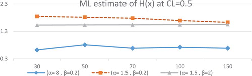
Figure 2. $\hat{H}\left(x\right)$ at different values of parameters for different sample size at CL = 0.7.

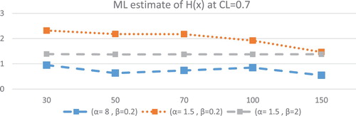
Figure 3. MSE of $\hat{H}\left(x\right)$ at different values of parameters for different sample size at CL = 0.5.

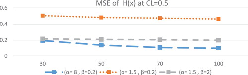
Figure 4. MSE of $\hat{H}\left(x\right)$ at different values of parameters for different sample size at CL = 0.7.

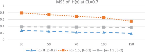
Table 1. Rbias, MSE, AL and CP of Entropy estimates at CL = 0.5.

	(α =  8, β = 0.2)						(α = 1.5, β = 0.2)						(α =  1.5, β = 2)
n	Exact value	Estimate	Rbias	MSE	AL	CP	Exact value	estimate	Rbias	MSE	AL	CP	Exact value	estimate	Rbias	MSE	AL	CP
30		0.622	0.056	0.195	0.689	0.959		1.845	0.398	0.505	1.324	0.92		1.528	0.231	0.215	0.21	0.935
50		0.809	0.228	0.139	0.639	0.951		1.815	0.375	0.482	1.264	0.922		1.535	0.227	0.208	0.155	0.93
70	0.659	0.685	0.039	0.109	0.638	0.979	1.32	1.78	0.348	0.474	0.656	0.98	1.987	1.538	0.226	0.204	0.131	0.951
100		0.72	0.093	0.1	0.634	0.976		1.695	0.284	0.463	0.607	0.985		1.543	.223	0.199	0.088	0.945
150		0.686	0.04	0.1	0.617	0.968		1.629	0.234	0.457	0.553	0.99		1.548	.221	0.193	0.059	0.947

Table 2. Rbias, MSE, AL and CP of Entropy estimates at CL = 0.7.

	(α = 8, β = 0.2)						(α = 1.5, β = 0.2)						(α = 1.5, β = 2)
N	Exact value	estimate	Rbias	MSE	AL	CP	Exact value	Estimate	Rbias	MSE	AL	CP	Exact value	estimate	Rbias	MSE	AL	CP
30		0.949	0.44	0.275	0.392	0.972		2.32	0.345	0.793	0.543	0.982		1.387	0.302	0.381	0.143	0.945
50		0.633	0.039	0.253	0.318	0.981		2.18	0.322	0.741	0.369	0.985		1.372	0.304	0.378	0.130	0.94
70	0.659	0.737	0.119	0.225	0.178	0.986	1.32	2.175	0.648	0.692	0.333	0.99	1.987	1.375	0.308	0.375	0.097	0.952
100		0.848	0.286	0.224	0.169	0.974		1.922	0.456	0.653	0.273	0.99		1.376	0.307	0.373	0.084	0.948
150		0.546	0.172	0.189	0.167	0.982		1.468	0.112	0.549	0.151	0.99		1.379	0.306	0.37	0.049	0.953

Figures 1 and 2 describe the ML estimates of $H\left(x\right)$. The following conclusions can be observed:

• The ML estimates of $H\left(x\right)$ decrease as the value of scale parameter $\beta$ increases for fixed value of shape parameter α.

• The ML estimates of $H\left(x\right)$ decrease as the parameter $\alpha$ increases for fixed value of parameter $\beta$.

• The ML estimates of $H\left(x\right)$ for α=8, $\beta$=0.2 have the smallest value compared with the corresponding estimates of the other sets of parameters.

• The ML estimates of $H\left(x\right)$ at CL = 0.5 approaches the true value than the ML estimates of $H\left(x\right)$ at CL = 0.7

Figures 3 and 4 describe the MSE of ML estimates for $H\left(x\right)$. The following conclusions can be observed in the properties of the ML estimates for $H\left(x\right)$ as follows:

• The MSE of ML estimates for $H\left(x\right)$ decreases as the sample size increases.

• For fixed value of scale parameter $\beta$, the MSE of $\hat{H}\left(x\right)$ decreases as the value of parameter $\alpha$ increases.

• For fixed value of shape parameter $\alpha$, the MSE of $\hat{H}\left(x\right)$ decreases as the value of parameter $\beta$ increases.

• The MSE of ML estimates of $\hat{H}\left(x\right)$ at α = 8, $\beta$ = 0.2 has the smallest value compared to the MSE of ML estimates for the corresponding other sets of parameters.

• The MSE of $\hat{H}\left(x\right)$ at CL = 0.5 is smaller than the MSE of $\hat{H}\left(x\right)$ at CL = 0.7.

Generally as seen from above tables that the coverage probabilities is very close to their corresponding nominal levels in approximately most cases. The maximum likelihood of entropy estimates decreases as the scale parameter of distribution decreases.

4.3. Real life data

The real-life data are a failure time of aircraft windshields that given by Blischke and Murthy [28]. They prove that the IW distribution fits this data. The failure time of aircraft windshields that measured in 1000 h are listed as follows (Table 3).

Table 3. Failure time of aircraft windshields (1000 h).

0.301	1.432	1.795	2.085	2.3	2.688	3.117	3.699	4.376
0.309	1.48	1.866	2.089	2.324	2.823	3.166	3.779	4.449
0.557	1.505	1.876	2.097	2.349	2.89	3.344	3.924	4.485
0.943	1.506	1.899	2.135	2.385	2.902	3.376	4.035	4.57
1.07	1.568	1.911	2.154	2.481	2.934	3.385	4.121	4.602
1.124	1.615	1.912	2.19	2.61	2.962	3.443	4.167	4.663
1.248	1.619	1.914	2.194	2.625	2.964	3.467	4.24	4.694
1.281	1.652	1.981	2.223	2.632	3.0	3.478	4.255
1.281	1.652	2.01	2.224	2.646	3.103	3.578	4.278
1.303	1.757	2.038	2.229	2.661	3.114	3.595	4.305

Using this data to estimate the entropy at CL = 0.7, 0.5 and complete sample (i.e. CL = 0). We find that $\hat{H}\left(x\right)=3.95$ at CL = 0.7, $\hat{H}\left(x\right)=3.185$ at CL = 0.5 and $\hat{H}\left(x\right)=2.513$ in case of complete sample.

5. Conclusion

This paper provides an estimation of Shanon entropy for inverse Weibull distribution using multiple censored data. The maximum likelihood estimators and approximate two-sided confidence limits of entropy are obtained. The performance of the entropy estimators for IW distribution is investigated in terms of their relative bias, mean square error, average length and coverage probability. Application to real data and simulation issues are provided.

From simulation results we conclude that, as the sample size increases, the mean square error of estimated entropy decreases. Regarding the average length of estimators, it can be observed that, as a sample size increases the length of the interval of ML estimate of entropy decreases and coverage probability increases. As censoring level increases, the mean square error of entropy estimate increases.

Disclosure statement

No potential conflict of interest was reported by the authors.

ORCID

Ahmed N. Zaky http://orcid.org/0000-0002-2236-4935

References

- Cover TM, Thomas JA. Elements of information theory. Hoboken (NJ): Wiley; 2005.
- Wong KM, Chan S. The entropy of ordered sequences and order statistics. IEEE Trans Inf Theory. 1990;36:276–284. doi: 10.1109/18.52473
- Morabbi H, Razmkhah M. Entropy of hybrid censoring schemes. J. Statist Res. 2010;6(2):161–176. doi: 10.18869/acadpub.jsri.6.2.161
- Abo-Eleneen ZA. The entropy of progressively censored samples. Entropy. 2011;13:437–449. DOI:10.3390/e13020437.
- Cho Y, Sun H, Lee K. An estimation of the entropy for a Rayleigh distribution based on doubly generalized Type-II hybrid censored samples. Entropy. 2014;16:3655–3669. DOI:10.3390/e16073655.
- Cho Y, Sun H, Lee K. Estimating the entropy of a Weibull distribution under generalized progressive hybrid censoring. Entropy. 2015;17(1):102–122. DOI:10.3390/e17010102.
- Lee K. Estimation of entropy of the inverse Weibull distribution under generalized progressive hybrid censored data. J Korea Inf Sci Soc. 2017;28(3):659–668. DOI:10.7465/jkdi.2017.28.3.659.
- Bader A. On the entropy of progressive hybrid censoring schemes. Appl Math Inf Sci. 2017;11(6):1811–1814. DOI:10.18576/amis/110629.
- Manoj C, Asha PS. Estimation of entropy for generalized exponential distribution based on record values. J Indian Soc Probab Stat. 2018;19(1):79–96. DOI:10.1007/s41096-018-0033-4.
- Lee NS, Jung ES, Bae JJ, et al. Uncertainty of agricultural product prices by information entropy model using probability distribution for monthly prices. J Korean Soc Agric Eng. 2012;54(2):7–14. DOI:10.5389/KSAE.2012.54.2.007.
- Chang DE, Ha KR, Jun HD, et al. Determination of optimal pressure monitoring locations of water distribution systems using entropy theory and genetic algorithm. J Korean Soc Water Wastewater. 2012;26(1):1–12. www.jksww.or.kr/journal/article.php?code=18843. doi: 10.11001/jksww.2012.26.1.001
- Rass S, König S. Password security as a game of entropies. Entropy. 2018;20:312. DOI:10.3390/e20050312.
- Rashidi S, Akar S, Bovand M, et al. Volume of fluid model to simulate the nanofluid flow and entropy generation in a single slope solar still. Renewable Energy. 2018;115:400–410. DOI:10.1016/j.renene.2017.08.059.
- Ellahi R, Alamri SZ, Basit A, et al. Effects of MHD and slip on heat transfer boundary layer flow over a moving plate based on specific entropy generation. J Taibah Univ Sci. 2018;12(4):476–482. DOI:10.1080/16583655.2018.1483795.
- Shehzad N, Zeeshan A, Ellahi R, et al. Modelling study on internal energy loss due to entropy generation for non-darcy poiseuille flow of silver-water nanofluid: an application of purification. Entropy. 2018;20(11):851. DOI:10.3390/e20110851.
- Bhatti MM, Abbas T, Rashidi MM, et al. Numerical simulation of entropy generation with thermal radiation on MHD carreau nanofluid towards a shrinking sheet. Entropy. 2016;18:200. DOI:10.3390/e18060200.
- Esfahani JA, Akbarzadeh M, Rashidi S, et al. Influences of wavy wall and nanoparticles on entropy generation over heat exchanger plat. Int J Heat Mass Transf. 2017;109(1):1162–1171. DOI:10.1016/j.ijheatmasstransfer.2017.03.006.
- Mamourian M, Shirvan KM, Ellahi R, et al. Optimization of mixed convection heat transfer with entropy generation in a wavy surface square lid-driven cavity by means of Taguchi approach. Int J Heat Mass Transf. 2016;102:544–554. DOI:10.1016/j.ijheatmasstransfer.2016.06.056.
- Bhatti MM, Abbas T, Rashidi MM, et al. Entropy generation on MHD eyring–powell Nanofluid through a permeable stretching surface. Entropy. 2016;18(6):224. DOI:10.3390/e18060224.
- Tobias PA, Trindade DC. Applied reliability. 2nd ed. New York: Chapman and Hall/CRC; 1995.
- Keller AZ, Giblin MT, Farnworth NR. Reliability analysis of commercial vehicle engines. Reliab Eng. 1985;10(1):15–25. DOI:10.1016/0143-8174(85)90039-3.
- Calabria R, Pulcini G. Bayes 2-sample prediction for the inverse Weibull distribution. Commun Stat Theory Methods. 1994;23(6):1811–1824. DOI:10.1080/03610929408831356.
- Jiang R, Murthy DNP, Ping JI. Models involving two inverse Weibull distributions. Reliab Eng Syst Safe. 2001;73(1):73–81. DOI:10.1016/S0951-8320(01)00030-8.
- Sultan KS. Bayesian estimates based on record values from the inverse Weibull lifetime model. Qual Technol Quant Manag. 2008;5:363–374. DOI:10.1080/16843703.2008.11673408.
- Kundu D, Howlader H. Bayesian inference and prediction of the inverse Weibull distribution for type-II censored data. Comput Stat Data Anal. 2010;54:1547–1558. DOI:10.1016/j.csda.2010.01.003.
- Hassan AS, Al-Thobety AK. Optimal design of failure step stress partially accelerated life tests with type II censored inverted Weibull data. IJERA. 2012;2(3):3242–3253.
- Hassan AS, Assar MS, Zaky AN. Constant-stress partially accelerated life tests for inverted Weibull distribution with multiple censored data. IJASP. 2015;3(1):72–82. DOI:10.14419/ijasp.v3i1.4418.
- Blischke WR, Murthy DNP. Reliability: modeling, prediction, and optimization. New York: Wiley; 2000.