New operational matrices of orthogonal Legendre polynomials and their operational

Abstract

Many conventional physical and engineering phenomena have been identified to be well expressed by making use of the fractional order partial differential equations (FOPDEs). For that reason, a proficient and stable numerical method is needed to find the approximate solution of FOPDEs. This article is designed to develop the numerical scheme able to find the approximate solution of generalized fractional order coupled systems (FOCSs) with mixed partial derivative terms of fractional order. Our main objective in this article is the development of a new operational matrix for fractional mixed partial derivatives based on the orthogonal shifted Legendre polynomials (SLPs). The fractional derivatives are considered herein in the sense of Caputo. The proposed method has the advantage to reduce the considered problems to a system of algebraic equations which are simple in handling by any computational software. Being easily solvable, the associated algebraic system leads to finding the solution of the problem. Some examples are included to demonstrate the accuracy and validity of the proposed method.

Keywords:

• Operational matrices of fractional order
• generalized fractional coupled systems
• Riemann-Liouville fractional integral
• Caputo fractional derivative
• orthogonal shifted Legendre polynomials

AMS Classifications:

• 26A33
• 35R11

1. Introduction

For the last few decades, the subject fractional calculus (FC) has gotten considerable attention of the researchers round the globe due to its non-local behaviour. For that reason, various conventional physical and engineering phenomena have found to be well described by making use of FC. The applications of FC has been observed in the fluid-dynamic traffic model, nonlinear oscillation of earthquakes, viscoelasticity, biomedical engineering, dynamics of interfaces between nano-particles and substrates, anomalous transport, and control theory, see for example [1–7], and references therein.

Owing to the formulation of many developed models in terms of fractional derivatives and integrals there is a strong need of the stable and efficient numerical methods to solve the problems consisting of derivatives and integrals of fractional order, i.e. fractional differential equations (FDEs). In recent years, several methods have been developed to solve FDEs, FOPDEs, and dynamic systems formulated using mathematical tools from FC. The names of few of them are Galerkin method [8], collocation method [9], Adomian's decomposition method [10,11], and operational matrices approach [12–21].

Orthogonal functions play a very important role in the development of the numerical methods for solving various types of problems. The solutions of many problems appearing in the various field of science have been approximated with the help of an orthogonal family of basis functions. The prime idea behind the technique of applying an orthogonal basis is that it reduces the under consideration problem into a system of algebraic equations, thus greatly simplifying the problem and simple in handling using any computational software. In this approach, a truncated orthogonal series is used for numerical integration of differential equations, with the goal of obtaining efficient computational solutions. The applications of orthogonal SLPs have been discussed in several existing articles [12,14,22,23].

In this study, we are eager to extend the applications of orthogonal SLPs to solve generalized FOCSs with mixed partial derivative terms of fractional order employing operational matrices approach. The differential equations consisting of mixed partial derivative terms are used to describe the very important physical phenomena: the flow through fissured rock [24], and the shearing motion of a fluid of second grade [25].

It is worth mentioning that the operational matrix for mixed partial derivatives of fractional order is not to be developed yet using SLPs along-with the use of fractional derivative in Caputo sense. In this study, we also address this research gap by developing the following result: (1) $\frac{{\mathrm{\partial }}^{\eta }}{\mathrm{\partial }{x}^{\left(\eta /2\right)}\mathrm{\partial }{y}^{\left(\eta /2\right)}}\left({\mathbf{\Lambda }}_{N^2}\right(x,y\left)\right)\simeq {\mathbf{D}}_{N^2\times N^2}^{\eta ,x,y}{\mathbf{\Lambda }}_{N^2}(x,y),$(1) where ${\mathbf{D}}_{N^2\times N^2}^{\eta ,x,y}$ is the operational matrix of mixed partial derivatives of order η studied in Section 3, and ${\mathbf{\Lambda }}_{N^2}(x,y)$ indicates the column vector of dimensions $N^2\times 1$, defined as $\begin{array}{rl}{\mathbf{\Lambda }}_{N^2}(x,y)& =\left[S_1\right(x\left)S_1\right(y),S_1(x\left)S_2\right(y),\dots ,S_1(x\left)S_N\right(y),\\ & S_2\left(x\right)S_1\left(y\right),S_2\left(x\right)S_2\left(y\right),\dots ,S_2\left(x\right)S_N\left(y\right),\\ & \cdots ,S_N\left(x\right)S_1\left(y\right),S_N\left(x\right)S_2\left(y\right),\dots ,\\ & S_N\left(x\right)S_N\left(y\right){]}^{\mathrm{T}},\end{array}$ where $S_l\left(x\right)$ and $S_k\left(y\right)$ with $l,m=0,1,\dots ,n$ are orthogonal SLPs [14].

The rest of the article is organized as follows: Some mathematical preliminaries and necessary definitions of FC theory and orthogonal SLPs which are necessary to develop the operational matrices are mentioned in Section 2. The Legendre operational matrices (LOMs) of fractional derivatives and integrals are obtained in Section 3. Section 4 is devoted to applying LOMs for finding the approximate solutions of generalized FOCSs. In Section 5, the convergence analysis of the proposed method is investigated. In Section 6, the proposed method is applied to several illustrative examples to check its validity and applicability. Also a conclusion is given in Section 7.

2. Preliminary remarks on FC

The subject FC has an advantage over integer order calculus being its generalization and is able to treat a wider class of the problems. The unique definition of the fractional differential operator does not exist: The frequently used are proposed by Riemann–Liouville (RL) and Caputo [26]. Unlike the Caputo proposed definition, the RL definition has certain limitations when trying to model the real-world phenomena with FDEs. Therefore in this study, we present the fractional differential operator proposed by Caputo [27].

Definition 2.1

RL fractional-order integral is given by (2) $J^{\eta }g\left(t\right)=\left\{\begin{array}{ll}\frac{1}{\mathit{\Gamma }\left(\eta \right)}{\int }_a^t(t-s{)}^{\eta -1}g(s)\mathrm{d}s,& \eta >0,\\ g\left(t\right),& \eta =0.\end{array}\right.$(2)

Definition 2.2

Caputo fractional derivative is given by (3) ${\mathcal{D}}^{\eta }g\left(t\right)=\left\{\begin{array}{ll}\frac{{\mathrm{d}}^{n}g\left(t\right)}{\mathrm{d}{t}^n},& \eta =n\in \\ & \{1,2,3,\dots \},\\ \frac{1}{\mathrm{\Gamma }(n-\eta )}\\ \times {\int }_a^t\frac{g^{\left(n\right)}\left(t\right)}{(t-s{)}^{\eta +1-n}}\mathrm{d}s,& n-1<\eta <n,\\ & n\in \{1,2,3,\dots \}.\end{array}\right.$(3)

The following well known properties of Caputo fractional derivative are proved in [28]: (4) $\begin{array}{rl}& {\mathcal{D}}^{\eta }C=0,C\mathrm{is}\mathrm{a}\mathrm{constant}.\\ & {\mathcal{D}}^{\eta }{t}^{\mu }=\left\{\begin{array}{ll}0,& \mathrm{for}\mu \in \{0,1,2,\dots \},\\ \mathrm{and}\mu <\lceil \eta \rceil ,\\ \frac{\mathrm{\Gamma }(\mu +1)}{\mathrm{\Gamma }(\mu +1-\eta )}{t}^{\mu -\eta },& \mathrm{for}\mu \in \{0,1,2,\dots \},\mathrm{and}\mu \ge \lceil \eta \rceil ,\\ & \mathrm{or}\mu \notin \{1,2,\dots \},\mathrm{and}\mu >\lfloor \eta \rfloor .\end{array}\right.\end{array}$(4)

2.1. Some properties of SLPs

The following recurrence formulae is used to describe the Legendre polynomials (LPs) on the interval $[-1,1]$ (see [12]) (5) $\begin{array}{rl}& P_{l+1}\left(s\right)=\frac{1+2l}{1+l}s{P}_l\left(s\right)-\frac{l}{1+l}s{P}_{l-1}\left(s\right),\\ & l=1,2,\dots ,\\ \mathrm{with}& P_0\left(s\right)=1\mathrm{and}{P}_1\left(s\right)=s.\end{array}$(5) We are interested in using the LPs on the interval $[0,1]$ instead of $[-1,1]$. For this, by introducing the change of variable s=2x−1, the analytic form of SLPs in variable x can be expressed as (see [12]) (6) $S_l\left(x\right)=\sum _{i=0}^l(-1{)}^{l+i}\frac{(l+i)!}{(l-i)!}\frac{x^i}{\left(\right(i)!{)}^2}.$(6) The orthogonality expression can be described as (7) ${\int }_0^1{S}_l\left(x\right)S_k\left(x\right)\mathrm{d}x=\left\{\begin{array}{ll}0& \mathrm{if}l\ne k,\\ \frac{1}{1+2l}& \mathrm{if}l=k.\end{array}\right.$(7) Therefore, a function $g\left(x\right)\in C\left(\right[0,1\left]\right)$ can be written in the form of a generalized SLPs as (8) $\begin{array}{rl}& g\left(x\right)=\sum _{k=0}^{\mathrm{\infty }}{e}_k{S}_k\left(x\right),\\ \mathrm{with}& e_k=⟨g\left(x\right),S_k\left(x\right)⟩\\ & =(2l+1){\int }_0^{1}g\left(x\right)S_k\left(x\right),k=1,2,\dots .\end{array}$(8) For the practical use, only considering the first $(l+1)$-terms of SLPs, we have (9) $\begin{array}{rl}& g\left(x\right)\approx \sum _{k=0}^l{e}_k{S}_k\left(x\right)=E^{\mathrm{T}}\mathrm{\Lambda }\left(x\right),\\ \mathrm{with}& E^T=[e_0,e_1,\dots ,e_l],\\ \mathrm{and}& \mathrm{\Lambda }\left(x\right)=\left[S_0\right(x),S_1(x),\dots ,S_l(x){]}^{\mathrm{T}}.\end{array}$(9) On the same fashion, the SLPs in two variables can be written as (see [14]) (10) $\begin{array}{rl}{S}_m(x,y)& =S_l\left(x\right)S_k\left(y\right)\\ & =\sum _{i=0}^l\sum _{j=0}^k(-1{)}^{l+i+k+j}\\ & \times \frac{(l+i)!(k+j)!}{(l-i)!(k-j)!}\frac{x^i{y}^j}{\left(\right(i)!{)}^2(\left(j\right)!{)}^2},\\ & m=Nl+k+1,l=0,1,2,\dots ,n,\\ & k=0,1,2,\dots ,n.\end{array}$(10) The orthogonality expression can be described as (11) $\begin{array}{rl}& {\int }_0^1{\int }_0^1{S}_l\left(x\right)S_k\left(y\right)S_q\left(x\right)S_p\left(y\right)\mathrm{d}x\mathrm{d}y\\ & =\left\{\begin{array}{ll}0& \mathrm{if}l\ne q,k\ne p\\ \frac{1}{(2l+1)(2k+1)}& \mathrm{if}l=q,k=p.\end{array}\right.\end{array}$(11) Therefore, a function $g(x,y)\in C\left(\right[0,1\left]\right)\times [0,1])$ can be written in the form of a generalized SLPs as (12) $\begin{array}{rl}& g(x,y)=\sum _{k=0}^{\mathrm{\infty }}\sum _{l=0}^{\mathrm{\infty }}{e}_{lk}{S}_m(x,y),\\ \mathrm{with}& e_{lk}=(2k+1)(2l+1)\\ & \times {\int }_0^1{\int }_0^{1}g(x,y)S_l\left(x\right)S_k\left(y\right)\mathrm{d}x\mathrm{d}y.\end{array}$(12) Equation (12(12) $\begin{array}{rl}& g(x,y)=\sum _{k=0}^{\mathrm{\infty }}\sum _{l=0}^{\mathrm{\infty }}{e}_{lk}{S}_m(x,y),\\ \mathrm{with}& e_{lk}=(2k+1)(2l+1)\\ & \times {\int }_0^1{\int }_0^{1}g(x,y)S_l\left(x\right)S_k\left(y\right)\mathrm{d}x\mathrm{d}y.\end{array}$(12) ) can also be described as (13) $\begin{array}{rl}& g(x,y)\approx \sum _{m=1}^{N^2}{e}_m{S}_m(x,y)={\mathbf{E}}^{\mathrm{T}}\mathbf{\Lambda }(x,y),\\ & e_m=e_{lk},m=Nl+k+1,\\ \mathrm{with}& {\mathbf{E}}^T=[e_{11},e_{12},\dots ,e_{1N},e_{21},e_{22},\\ & \dots ,e_{2N},\dots ,e_{N1},e_{N2},\dots ,e_{NN}],\\ \mathrm{and}& \mathbf{\Lambda }(x,y)=\left[S_1\right(x\left)S_1\right(y),S_1(x\left)S_2\right(y),\dots ,\\ & S_1\left(x\right)S_N\left(y\right),S_2\left(x\right)S_1\left(y\right),S_2\left(x\right)S_2\left(y\right),\\ & \cdots ,S_2\left(x\right)S_N\left(y\right),\dots ,S_N\left(x\right)S_1\left(y\right),S_N\left(x\right)\\ & S_2\left(y\right),\dots ,S_N\left(x\right)S_N\left(y\right){]}^{\mathrm{T}}.\end{array}$(13)

Lemma 2.3

Let $\mathbf{\Lambda }(x,y)$ be the shifted Legendre function vector in two variables defined in (13(13) $\begin{array}{rl}& g(x,y)\approx \sum _{m=1}^{N^2}{e}_m{S}_m(x,y)={\mathbf{E}}^{\mathrm{T}}\mathbf{\Lambda }(x,y),\\ & e_m=e_{lk},m=Nl+k+1,\\ \mathrm{with}& {\mathbf{E}}^T=[e_{11},e_{12},\dots ,e_{1N},e_{21},e_{22},\\ & \dots ,e_{2N},\dots ,e_{N1},e_{N2},\dots ,e_{NN}],\\ \mathrm{and}& \mathbf{\Lambda }(x,y)=\left[S_1\right(x\left)S_1\right(y),S_1(x\left)S_2\right(y),\dots ,\\ & S_1\left(x\right)S_N\left(y\right),S_2\left(x\right)S_1\left(y\right),S_2\left(x\right)S_2\left(y\right),\\ & \cdots ,S_2\left(x\right)S_N\left(y\right),\dots ,S_N\left(x\right)S_1\left(y\right),S_N\left(x\right)\\ & S_2\left(y\right),\dots ,S_N\left(x\right)S_N\left(y\right){]}^{\mathrm{T}}.\end{array}$(13) ), and also assume that $\eta >0,$ then (14) $J^{\eta }\mathbf{\Lambda }(x,y)\simeq {\mathbf{Q}}^{\left(\eta \right)}\mathbf{\Lambda }(x,y),$(14) where ${\mathbf{Q}}^{\left(\eta \right)}$ is the $N^2\times N^2$ operational matrix of fractional integration of order η studied in [14].

Lemma 2.4

Let $\mathbf{\Lambda }(x,y)$ be the shifted Legendre function vector in two variables defined in (13(13) $\begin{array}{rl}& g(x,y)\approx \sum _{m=1}^{N^2}{e}_m{S}_m(x,y)={\mathbf{E}}^{\mathrm{T}}\mathbf{\Lambda }(x,y),\\ & e_m=e_{lk},m=Nl+k+1,\\ \mathrm{with}& {\mathbf{E}}^T=[e_{11},e_{12},\dots ,e_{1N},e_{21},e_{22},\\ & \dots ,e_{2N},\dots ,e_{N1},e_{N2},\dots ,e_{NN}],\\ \mathrm{and}& \mathbf{\Lambda }(x,y)=\left[S_1\right(x\left)S_1\right(y),S_1(x\left)S_2\right(y),\dots ,\\ & S_1\left(x\right)S_N\left(y\right),S_2\left(x\right)S_1\left(y\right),S_2\left(x\right)S_2\left(y\right),\\ & \cdots ,S_2\left(x\right)S_N\left(y\right),\dots ,S_N\left(x\right)S_1\left(y\right),S_N\left(x\right)\\ & S_2\left(y\right),\dots ,S_N\left(x\right)S_N\left(y\right){]}^{\mathrm{T}}.\end{array}$(13) ), and also assume that $\eta >0,$ then (15) ${\mathcal{D}}_x^{\eta }\mathbf{\Lambda }(x,y)\simeq {\mathbf{D}}^{\left(\eta \right)}\mathbf{\Lambda }(x,y),$(15) where ${\mathbf{D}}^{\left(\eta \right)}$ is the $N^2\times N^2$ operational matrix of fractional derivative of order η in the Caputo sense studied in [14].

3. Main results

In this section, we generalize the operational matrix for fractional derivatives of SLPs able to find the numerical solution of generalized FOCSs with mixed partial derivative terms of fractional order.

Theorem 3.1

Let ${\mathbf{\Lambda }}_{N^2}(x,y)$ be the shifted Legendre function vector of dimensions $N^2\times 1$, defined in (13(13) $\begin{array}{rl}& g(x,y)\approx \sum _{m=1}^{N^2}{e}_m{S}_m(x,y)={\mathbf{E}}^{\mathrm{T}}\mathbf{\Lambda }(x,y),\\ & e_m=e_{lk},m=Nl+k+1,\\ \mathrm{with}& {\mathbf{E}}^T=[e_{11},e_{12},\dots ,e_{1N},e_{21},e_{22},\\ & \dots ,e_{2N},\dots ,e_{N1},e_{N2},\dots ,e_{NN}],\\ \mathrm{and}& \mathbf{\Lambda }(x,y)=\left[S_1\right(x\left)S_1\right(y),S_1(x\left)S_2\right(y),\dots ,\\ & S_1\left(x\right)S_N\left(y\right),S_2\left(x\right)S_1\left(y\right),S_2\left(x\right)S_2\left(y\right),\\ & \cdots ,S_2\left(x\right)S_N\left(y\right),\dots ,S_N\left(x\right)S_1\left(y\right),S_N\left(x\right)\\ & S_2\left(y\right),\dots ,S_N\left(x\right)S_N\left(y\right){]}^{\mathrm{T}}.\end{array}$(13) ), then (16) $\frac{{\mathrm{\partial }}^{\eta }}{\mathrm{\partial }{x}^{\left(\eta /2\right)}\mathrm{\partial }{y}^{\left(\eta /2\right)}}\mathbf{\Lambda }(x,y)\simeq {\mathbf{D}}^{\eta ,x,y}\mathbf{\Lambda }(x,y),$(16) where ${\mathbf{D}}^{\eta ,x,y}$ is the $N^2\times N^2$ operational matrix of mixed partial derivatives of fractional order η in the Caputo sense and is defined as follows: ${\mathbf{D}}^{\eta ,x,y}=\left(\begin{array}{cccccc}{\mathrm{\Theta }}_{1,1,n}& {\mathrm{\Theta }}_{1,2,n}& \cdots & {\mathrm{\Theta }}_{1,w,n}& \cdots & {\mathrm{\Theta }}_{1,N^2,n}\\ {\mathrm{\Theta }}_{2,1,n}& {\mathrm{\Theta }}_{2,2,n}& \cdots & {\mathrm{\Theta }}_{2,w,n}& \cdots & {\mathrm{\Theta }}_{2,N^2,n}\\ ⋮& ⋮& ⋮& ⋮& ⋮& ⋮\\ {\mathrm{\Theta }}_{c,1,n}& {\mathrm{\Theta }}_{c,2,n}& \cdots & {\mathrm{\Theta }}_{c,w,n}& \cdots & {\mathrm{\Theta }}_{c,N^2,n}\\ ⋮& ⋮& ⋮& ⋮& ⋮& ⋮\\ {\mathrm{\Theta }}_{N^2,1,n}& {\mathrm{\Theta }}_{N^2,2,n}& \cdots & {\mathrm{\Theta }}_{N^2,w,n}& \cdots & {\mathrm{\Theta }}_{N^2,N^2,n}\end{array}\right),$ where $w=N{k}^{\prime }+l^{\prime }+1,c=Nk+l+1,\mathrm{for}k,l,k^{\prime },l^{\prime }=0,1,2,\dots ,n,$ ${\mathrm{\Theta }}_{(i,j,w,c)}=\sum _{i=\lceil \eta /2\rceil }^l\sum _{j=\lceil \eta /2\rceil }^k{A}_{(i,k)}{B}_{(j,l)}\overbrace{\underset{(i,j,\eta )}{\mathrm{\Omega }}}{e}_{(l^{\prime },k^{\prime },i^{\prime },j^{\prime },\eta )},$ with $\begin{array}{rl}{e}_{(l^{\prime },k^{\prime },i^{\prime },j^{\prime },\eta )}& ={\delta }_{i^{\prime },j^{\prime },w,c}(2i^{\prime }+1)(2j^{\prime }+1)\sum _{i^{\prime }=0}^{l^{\prime }}\sum _{j^{\prime }=0}^{k^{\prime }}{A}_{(i^{\prime },l^{\prime })}{B}_{(j^{\prime },k^{\prime })}\\ & \times \frac{1}{(i+i^{\prime }-\eta /2+1)(j+j^{\prime }-\eta /2+1)},\\ A_{(i^{\prime },l^{\prime })}& =\frac{(-1{)}^{l^{\prime }+i^{\prime }}(l^{\prime }+i^{\prime })!}{(l^{\prime }-i^{\prime })!(l^{\prime }!{)}^2},B_{(j^{\prime },k^{\prime })}\\ & =\frac{(-1{)}^{k^{\prime }+j^{\prime }}(k^{\prime }+j^{\prime })!}{(k^{\prime }-j^{\prime })!(k^{\prime }!{)}^2},\end{array}$ and (17) $\overbrace{\underset{(i,j,\eta )}{\mathrm{\Omega }}}=\frac{\mathrm{\Gamma }(i+1)\mathrm{\Gamma }(j+1)}{\mathrm{\Gamma }(i+1-\eta /2)\mathrm{\Gamma }(j+1-\eta /2)}.$(17)

Proof.

Using Equations (4(4) $\begin{array}{rl}& {\mathcal{D}}^{\eta }C=0,C\mathrm{is}\mathrm{a}\mathrm{constant}.\\ & {\mathcal{D}}^{\eta }{t}^{\mu }=\left\{\begin{array}{ll}0,& \mathrm{for}\mu \in \{0,1,2,\dots \},\\ \mathrm{and}\mu <\lceil \eta \rceil ,\\ \frac{\mathrm{\Gamma }(\mu +1)}{\mathrm{\Gamma }(\mu +1-\eta )}{t}^{\mu -\eta },& \mathrm{for}\mu \in \{0,1,2,\dots \},\mathrm{and}\mu \ge \lceil \eta \rceil ,\\ & \mathrm{or}\mu \notin \{1,2,\dots \},\mathrm{and}\mu >\lfloor \eta \rfloor .\end{array}\right.\end{array}$(4) ), (10(10) $\begin{array}{rl}{S}_m(x,y)& =S_l\left(x\right)S_k\left(y\right)\\ & =\sum _{i=0}^l\sum _{j=0}^k(-1{)}^{l+i+k+j}\\ & \times \frac{(l+i)!(k+j)!}{(l-i)!(k-j)!}\frac{x^i{y}^j}{\left(\right(i)!{)}^2(\left(j\right)!{)}^2},\\ & m=Nl+k+1,l=0,1,2,\dots ,n,\\ & k=0,1,2,\dots ,n.\end{array}$(10) ) and the linear property of the Caputo differential operator, we have (18) $\begin{array}{rl}& \frac{{\mathrm{\partial }}^{\eta }}{\mathrm{\partial }{x}^{\left(\eta /2\right)}\mathrm{\partial }{y}^{\left(\eta /2\right)}}{S}_m(x,y)\\ & =\sum _{i=\lceil \eta /2\rceil }^l\sum _{j=\lceil \eta /2\rceil }^k{A}_{(i,l)}{B}_{(j,k)}\overbrace{\underset{(i,j,\eta )}{\mathrm{\Omega }}}{x}^{i-\eta /2}{y}^{j-\eta /2},\\ \mathrm{where}& A_{(i,l)}=(-1{)}^{l+i}\frac{(l+i)!}{(l-i)!}\frac{1}{\left(\right(i)!{)}^2},\\ & B_{(j,k)}=(-1{)}^{k+j}\frac{(k+j)!}{(k-j)!}\frac{1}{\left(\right(j)!{)}^2},\\ \mathrm{and}& \overbrace{\underset{(i,j,\eta )}{\mathrm{\Omega }}}=\frac{\mathrm{\Gamma }(i+1)\mathrm{\Gamma }(j+1)}{\mathrm{\Gamma }(i+1-\eta /2)\mathrm{\Gamma }(j+1-\eta /2)}.\end{array}$(18) Approximating $x^{i-\eta /2}{y}^{j-\eta /2}$ with SLPs, we have (19) $x^{i-\eta /2}{y}^{j-\eta /2}=\sum _{i^{\prime }=0}^m\sum _{j^{\prime }=0}^m{e}_{(l^{\prime },k^{\prime },i^{\prime },j^{\prime },\eta )}{S}_{i^{\prime }}\left(x\right)S_j^{\prime }\left(y\right),$(19) where (20) $\begin{array}{rl}& e_{(l^{\prime },k^{\prime },i^{\prime },j^{\prime },\eta )}=(2i^{\prime }+1)(2j^{\prime }+1)\\ & \times {\int }_0^1{\int }_0^1{x}^{i-\eta /2}{y}^{j-\eta /2}{S}_{i^{\prime }}\left(x\right)S_{j^{\prime }}\left(y\right)\mathrm{d}x\mathrm{d}y.\end{array}$(20) Evaluating the integrals involved in Equation (20(20) $\begin{array}{rl}& e_{(l^{\prime },k^{\prime },i^{\prime },j^{\prime },\eta )}=(2i^{\prime }+1)(2j^{\prime }+1)\\ & \times {\int }_0^1{\int }_0^1{x}^{i-\eta /2}{y}^{j-\eta /2}{S}_{i^{\prime }}\left(x\right)S_{j^{\prime }}\left(y\right)\mathrm{d}x\mathrm{d}y.\end{array}$(20) ) and making use of Equation (10(10) $\begin{array}{rl}{S}_m(x,y)& =S_l\left(x\right)S_k\left(y\right)\\ & =\sum _{i=0}^l\sum _{j=0}^k(-1{)}^{l+i+k+j}\\ & \times \frac{(l+i)!(k+j)!}{(l-i)!(k-j)!}\frac{x^i{y}^j}{\left(\right(i)!{)}^2(\left(j\right)!{)}^2},\\ & m=Nl+k+1,l=0,1,2,\dots ,n,\\ & k=0,1,2,\dots ,n.\end{array}$(10) ), we have (21) $\begin{array}{rl}& e_{(l^{\prime },k^{\prime },i^{\prime },j^{\prime },\eta )}={\delta }_{i^{\prime },j^{\prime },w,c}(2i^{\prime }+1)(2j^{\prime }+1)\\ & \times \sum _{i^{\prime }=0}^{l^{\prime }}\sum _{j^{\prime }=0}^{k^{\prime }}{A}_{(i^{\prime },l^{\prime })}{B}_{(j^{\prime },k^{\prime })}\\ & \times \frac{1}{(i+i^{\prime }-\frac{\eta }{2}+1)(j+j^{\prime }-\frac{\eta }{2}+1)},\\ \mathrm{with}& A_{(i^{\prime },l^{\prime })}=(-1{)}^{l^{\prime }+i^{\prime }}\frac{(l^{\prime }+i^{\prime })!}{(l^{\prime }-i^{\prime })!}\frac{1}{\left(\right(i^{\prime })!{)}^2},\\ & B_{(j^{\prime },k^{\prime })}=(-1{)}^{k^{\prime }+j^{\prime }}\frac{(k^{\prime }+j^{\prime })!}{(k^{\prime }-j^{\prime })!}\frac{1}{\left(\right(j^{\prime })!{)}^2},\end{array}$(21) where ${\delta }_{i^{\prime },j^{\prime },w,c}=\left\{\begin{array}{ll}0& \mathrm{if}{i}^{\prime }\ne w,j^{\prime }\ne c,\\ 1& \mathrm{if}{i}^{\prime }=w,j^{\prime }=c.\end{array}\right.$ Substituting the Equations (19(19) $x^{i-\eta /2}{y}^{j-\eta /2}=\sum _{i^{\prime }=0}^m\sum _{j^{\prime }=0}^m{e}_{(l^{\prime },k^{\prime },i^{\prime },j^{\prime },\eta )}{S}_{i^{\prime }}\left(x\right)S_j^{\prime }\left(y\right),$(19) ), (21(21) $\begin{array}{rl}& e_{(l^{\prime },k^{\prime },i^{\prime },j^{\prime },\eta )}={\delta }_{i^{\prime },j^{\prime },w,c}(2i^{\prime }+1)(2j^{\prime }+1)\\ & \times \sum _{i^{\prime }=0}^{l^{\prime }}\sum _{j^{\prime }=0}^{k^{\prime }}{A}_{(i^{\prime },l^{\prime })}{B}_{(j^{\prime },k^{\prime })}\\ & \times \frac{1}{(i+i^{\prime }-\frac{\eta }{2}+1)(j+j^{\prime }-\frac{\eta }{2}+1)},\\ \mathrm{with}& A_{(i^{\prime },l^{\prime })}=(-1{)}^{l^{\prime }+i^{\prime }}\frac{(l^{\prime }+i^{\prime })!}{(l^{\prime }-i^{\prime })!}\frac{1}{\left(\right(i^{\prime })!{)}^2},\\ & B_{(j^{\prime },k^{\prime })}=(-1{)}^{k^{\prime }+j^{\prime }}\frac{(k^{\prime }+j^{\prime })!}{(k^{\prime }-j^{\prime })!}\frac{1}{\left(\right(j^{\prime })!{)}^2},\end{array}$(21) ) in Equation (18(18) $\begin{array}{rl}& \frac{{\mathrm{\partial }}^{\eta }}{\mathrm{\partial }{x}^{\left(\eta /2\right)}\mathrm{\partial }{y}^{\left(\eta /2\right)}}{S}_m(x,y)\\ & =\sum _{i=\lceil \eta /2\rceil }^l\sum _{j=\lceil \eta /2\rceil }^k{A}_{(i,l)}{B}_{(j,k)}\overbrace{\underset{(i,j,\eta )}{\mathrm{\Omega }}}{x}^{i-\eta /2}{y}^{j-\eta /2},\\ \mathrm{where}& A_{(i,l)}=(-1{)}^{l+i}\frac{(l+i)!}{(l-i)!}\frac{1}{\left(\right(i)!{)}^2},\\ & B_{(j,k)}=(-1{)}^{k+j}\frac{(k+j)!}{(k-j)!}\frac{1}{\left(\right(j)!{)}^2},\\ \mathrm{and}& \overbrace{\underset{(i,j,\eta )}{\mathrm{\Omega }}}=\frac{\mathrm{\Gamma }(i+1)\mathrm{\Gamma }(j+1)}{\mathrm{\Gamma }(i+1-\eta /2)\mathrm{\Gamma }(j+1-\eta /2)}.\end{array}$(18) ), we have (22) $\begin{array}{rl}& \frac{{\mathrm{\partial }}^{\eta }}{\mathrm{\partial }{x}^{\left(\eta /2\right)}\mathrm{\partial }{y}^{\left(\eta /2\right)}}{S}_m(x,y)=\sum _{i^{\prime }=0}^m\sum _{j^{\prime }=0}^m\sum _{i=\lceil \eta /2\rceil }^l\\ & \times \sum _{j=\lceil \eta /2\rceil }^k{A}_{(i^{\prime },l^{\prime })}{B}_{(j^{\prime },k^{\prime })}\overbrace{\underset{(i,j,\eta )}{\mathrm{\Omega }}}{e}_{(l^{\prime },k^{\prime },i^{\prime },j^{\prime },\eta )}{S}_{i^{\prime }}\left(x\right)S_{j^{\prime }}\left(y\right).\end{array}$(22) Let ${\mathrm{\Theta }}_{(i,j,w,c)}=\sum _{i=\lceil \eta /2\rceil }^l\sum _{j=\frac{\eta }{/}2\rceil }^k{A}_{(i,k)}{B}_{(j,l)}\overbrace{\underset{(i,j,\eta )}{\mathrm{\Omega }}}{e}_{(l^{\prime },k^{\prime },i^{\prime },j^{\prime },\eta )}.$ Then Equation (22(22) $\begin{array}{rl}& \frac{{\mathrm{\partial }}^{\eta }}{\mathrm{\partial }{x}^{\left(\eta /2\right)}\mathrm{\partial }{y}^{\left(\eta /2\right)}}{S}_m(x,y)=\sum _{i^{\prime }=0}^m\sum _{j^{\prime }=0}^m\sum _{i=\lceil \eta /2\rceil }^l\\ & \times \sum _{j=\lceil \eta /2\rceil }^k{A}_{(i^{\prime },l^{\prime })}{B}_{(j^{\prime },k^{\prime })}\overbrace{\underset{(i,j,\eta )}{\mathrm{\Omega }}}{e}_{(l^{\prime },k^{\prime },i^{\prime },j^{\prime },\eta )}{S}_{i^{\prime }}\left(x\right)S_{j^{\prime }}\left(y\right).\end{array}$(22) ) becomes (23) $\frac{{\mathrm{\partial }}^{\eta }}{\mathrm{\partial }{x}^{\left(\eta /2\right)}\mathrm{\partial }{y}^{\left(\eta /2\right)}}{S}_m(x,y)=\sum _{i^{\prime }=0}^m\sum _{j^{\prime }=0}^m{\mathrm{\Theta }}_{(i,j,w,c)}{S}_{i^{\prime }}\left(x\right)S_{j^{\prime }}\left(y\right).$(23) The desire result is obtained employing the notations $w=N{k}^{\prime }+l^{\prime }+1,c=Nk+l+1,k,l,k^{\prime },l^{\prime }=0,1,2,\dots ,n$.

4. Applications of the operational matrices of fractional order

In this section, we ensure the applicability of the operational matrices by developing the numerical scheme able to treat the generalized FOCSs of the type: (24) $\begin{array}{rl}\frac{{\mathrm{\partial }}^{{\eta }_m}}{\mathrm{\partial }{x}^{{\eta }_m}}{u}_1(x,y)& =\sum _{j=0}^{m-1}{a}_j\frac{{\mathrm{\partial }}^{\left({\eta }_j\right)}}{\mathrm{\partial }{y}^{{\eta }_j}}{u}_1(x,y)\\ & +\sum _{j=0}^{m^{\prime }-1}{b}_j\frac{{\mathrm{\partial }}^{\left({\vartheta }_j\right)}}{\mathrm{\partial }{x}^{{\vartheta }_j}}{u}_2(x,y)\\ & +\sum _{j=0}^{m^{\prime }-1}{c}_j\frac{{\mathrm{\partial }}^{\left({\vartheta }_j\right)}}{\mathrm{\partial }{y}^{{\vartheta }_j}}{u}_2(x,y)\\ & +\sum _{j=0}^{m^{\prime }-1}{d}_j\frac{{\mathrm{\partial }}^{\left({\kappa }_j\right)}}{\mathrm{\partial }{x}^{{\kappa }_j/2}\mathrm{\partial }{y}^{{\kappa }_j/2}}{u}_2(x,y)\\ & +\sum _{j=0}^{m-1}{e}_j\frac{{\mathrm{\partial }}^{\left({\varrho }_j\right)}}{\mathrm{\partial }{x}^{{\varrho }_j/2}\mathrm{\partial }{y}^{{\varrho }_j/2}}{u}_1(x,y)+f_1(x,y),\\ \frac{{\mathrm{\partial }}^{{\vartheta }_{m^{\prime }}}}{\mathrm{\partial }{x}^{{\vartheta }_{m^{\prime }}}}{u}_2(x,y)& =\sum _{j=0}^{m^{\prime }-1}{b}_j^{\prime }\frac{{\mathrm{\partial }}^{\left({\vartheta }_j\right)}}{\mathrm{\partial }{y}^{{\vartheta }_j}}{u}_2(x,y)\\ & +\sum _{j=0}^{m-1}{a}_j^{\prime }\frac{{\mathrm{\partial }}^{\left({\eta }_j\right)}}{\mathrm{\partial }{x}^{{\eta }_j}}{u}_1(x,y)\\ & +\sum _{j=0}^{m-1}{a}_j^{″}\frac{{\mathrm{\partial }}^{\left({\eta }_j\right)}}{\mathrm{\partial }{y}^{{\eta }_j}}{u}_1(x,y)\\ & +\sum _{j=0}^{m^{\prime }-1}{d}_j^{\prime }\frac{{\mathrm{\partial }}^{\left({\kappa }_j\right)}}{\mathrm{\partial }{x}^{{\kappa }_j/2}\mathrm{\partial }{y}^{{\kappa }_j/2}}{u}_2(x,y)\\ & +\sum _{j=0}^{m-1}{e}_j^{\prime }\frac{{\mathrm{\partial }}^{\left({\varrho }_j\right)}}{\mathrm{\partial }{x}^{{\varrho }_j/2}\mathrm{\partial }{y}^{{\varrho }_j/2}}{u}_1(x,y)+f_2(x,y),\end{array}$(24) subject to the initial conditions (25) $\begin{array}{rl}& u_1^{\left(j\right)}(0,y)=g_j\left(y\right),j=0,1,2,3\cdots m,\\ & u_2^{\left(j\right)}(0,y)=h_j\left(y\right),j=0,1,2,3\cdots m^{\prime },\end{array}$(25) where $a_j,a_j^{\prime },a_j^{″},b_j,b_j^{\prime },c_j,d_j,d_j^{\prime },e_j,e_j^{\prime }\in \mathbb{R}$, $u_1(x,y),u_2(x,y),f_1(x,y),f_2(x,y)$ are assumed to be continuous functions defined on the compact region $[0,1]\times [0,1]$, $0<{\eta }_0\le 1\cdots m<{\eta }_m\le m+1$, and ${\vartheta }_j,{\varrho }_j,{\kappa }_j$ are defined analogously. It is worth mentioning that the fractional derivatives in the problem (24(24) $\begin{array}{rl}\frac{{\mathrm{\partial }}^{{\eta }_m}}{\mathrm{\partial }{x}^{{\eta }_m}}{u}_1(x,y)& =\sum _{j=0}^{m-1}{a}_j\frac{{\mathrm{\partial }}^{\left({\eta }_j\right)}}{\mathrm{\partial }{y}^{{\eta }_j}}{u}_1(x,y)\\ & +\sum _{j=0}^{m^{\prime }-1}{b}_j\frac{{\mathrm{\partial }}^{\left({\vartheta }_j\right)}}{\mathrm{\partial }{x}^{{\vartheta }_j}}{u}_2(x,y)\\ & +\sum _{j=0}^{m^{\prime }-1}{c}_j\frac{{\mathrm{\partial }}^{\left({\vartheta }_j\right)}}{\mathrm{\partial }{y}^{{\vartheta }_j}}{u}_2(x,y)\\ & +\sum _{j=0}^{m^{\prime }-1}{d}_j\frac{{\mathrm{\partial }}^{\left({\kappa }_j\right)}}{\mathrm{\partial }{x}^{{\kappa }_j/2}\mathrm{\partial }{y}^{{\kappa }_j/2}}{u}_2(x,y)\\ & +\sum _{j=0}^{m-1}{e}_j\frac{{\mathrm{\partial }}^{\left({\varrho }_j\right)}}{\mathrm{\partial }{x}^{{\varrho }_j/2}\mathrm{\partial }{y}^{{\varrho }_j/2}}{u}_1(x,y)+f_1(x,y),\\ \frac{{\mathrm{\partial }}^{{\vartheta }_{m^{\prime }}}}{\mathrm{\partial }{x}^{{\vartheta }_{m^{\prime }}}}{u}_2(x,y)& =\sum _{j=0}^{m^{\prime }-1}{b}_j^{\prime }\frac{{\mathrm{\partial }}^{\left({\vartheta }_j\right)}}{\mathrm{\partial }{y}^{{\vartheta }_j}}{u}_2(x,y)\\ & +\sum _{j=0}^{m-1}{a}_j^{\prime }\frac{{\mathrm{\partial }}^{\left({\eta }_j\right)}}{\mathrm{\partial }{x}^{{\eta }_j}}{u}_1(x,y)\\ & +\sum _{j=0}^{m-1}{a}_j^{″}\frac{{\mathrm{\partial }}^{\left({\eta }_j\right)}}{\mathrm{\partial }{y}^{{\eta }_j}}{u}_1(x,y)\\ & +\sum _{j=0}^{m^{\prime }-1}{d}_j^{\prime }\frac{{\mathrm{\partial }}^{\left({\kappa }_j\right)}}{\mathrm{\partial }{x}^{{\kappa }_j/2}\mathrm{\partial }{y}^{{\kappa }_j/2}}{u}_2(x,y)\\ & +\sum _{j=0}^{m-1}{e}_j^{\prime }\frac{{\mathrm{\partial }}^{\left({\varrho }_j\right)}}{\mathrm{\partial }{x}^{{\varrho }_j/2}\mathrm{\partial }{y}^{{\varrho }_j/2}}{u}_1(x,y)+f_2(x,y),\end{array}$(24) ) are considered in Caputo sense.

4.1. Method of solution

The unknowns $u_1(x,y)$ and $u_2(x,y)$ is approximated by SLPs to compute the solution of the problem (24(24) $\begin{array}{rl}\frac{{\mathrm{\partial }}^{{\eta }_m}}{\mathrm{\partial }{x}^{{\eta }_m}}{u}_1(x,y)& =\sum _{j=0}^{m-1}{a}_j\frac{{\mathrm{\partial }}^{\left({\eta }_j\right)}}{\mathrm{\partial }{y}^{{\eta }_j}}{u}_1(x,y)\\ & +\sum _{j=0}^{m^{\prime }-1}{b}_j\frac{{\mathrm{\partial }}^{\left({\vartheta }_j\right)}}{\mathrm{\partial }{x}^{{\vartheta }_j}}{u}_2(x,y)\\ & +\sum _{j=0}^{m^{\prime }-1}{c}_j\frac{{\mathrm{\partial }}^{\left({\vartheta }_j\right)}}{\mathrm{\partial }{y}^{{\vartheta }_j}}{u}_2(x,y)\\ & +\sum _{j=0}^{m^{\prime }-1}{d}_j\frac{{\mathrm{\partial }}^{\left({\kappa }_j\right)}}{\mathrm{\partial }{x}^{{\kappa }_j/2}\mathrm{\partial }{y}^{{\kappa }_j/2}}{u}_2(x,y)\\ & +\sum _{j=0}^{m-1}{e}_j\frac{{\mathrm{\partial }}^{\left({\varrho }_j\right)}}{\mathrm{\partial }{x}^{{\varrho }_j/2}\mathrm{\partial }{y}^{{\varrho }_j/2}}{u}_1(x,y)+f_1(x,y),\\ \frac{{\mathrm{\partial }}^{{\vartheta }_{m^{\prime }}}}{\mathrm{\partial }{x}^{{\vartheta }_{m^{\prime }}}}{u}_2(x,y)& =\sum _{j=0}^{m^{\prime }-1}{b}_j^{\prime }\frac{{\mathrm{\partial }}^{\left({\vartheta }_j\right)}}{\mathrm{\partial }{y}^{{\vartheta }_j}}{u}_2(x,y)\\ & +\sum _{j=0}^{m-1}{a}_j^{\prime }\frac{{\mathrm{\partial }}^{\left({\eta }_j\right)}}{\mathrm{\partial }{x}^{{\eta }_j}}{u}_1(x,y)\\ & +\sum _{j=0}^{m-1}{a}_j^{″}\frac{{\mathrm{\partial }}^{\left({\eta }_j\right)}}{\mathrm{\partial }{y}^{{\eta }_j}}{u}_1(x,y)\\ & +\sum _{j=0}^{m^{\prime }-1}{d}_j^{\prime }\frac{{\mathrm{\partial }}^{\left({\kappa }_j\right)}}{\mathrm{\partial }{x}^{{\kappa }_j/2}\mathrm{\partial }{y}^{{\kappa }_j/2}}{u}_2(x,y)\\ & +\sum _{j=0}^{m-1}{e}_j^{\prime }\frac{{\mathrm{\partial }}^{\left({\varrho }_j\right)}}{\mathrm{\partial }{x}^{{\varrho }_j/2}\mathrm{\partial }{y}^{{\varrho }_j/2}}{u}_1(x,y)+f_2(x,y),\end{array}$(24) ) and (25(25) $\begin{array}{rl}& u_1^{\left(j\right)}(0,y)=g_j\left(y\right),j=0,1,2,3\cdots m,\\ & u_2^{\left(j\right)}(0,y)=h_j\left(y\right),j=0,1,2,3\cdots m^{\prime },\end{array}$(25) ), as (26) $\begin{array}{rl}\frac{{\mathrm{\partial }}^{{\eta }_m}}{\mathrm{\partial }{x}^{{\eta }_m}}{u}_1(x,y)& ={{\mathbf{E}}_{\mathbf{1}}}_{N^2}^{\mathrm{T}}{\mathbf{\Lambda }}_{N^2}(x,y),\\ \frac{{\mathrm{\partial }}^{{\vartheta }_{m^{\prime }}}}{\mathrm{\partial }{x}^{{\vartheta }_{m^{\prime }}}}{u}_2(x,y)& ={{\mathbf{E}}_{\mathbf{2}}}_{N^2}^{\mathrm{T}}{\mathbf{\Lambda }}_{N^2}(x,y).\end{array}$(26) In the light of Lemma 2.3 and making use of the initial conditions, (26(26) $\begin{array}{rl}\frac{{\mathrm{\partial }}^{{\eta }_m}}{\mathrm{\partial }{x}^{{\eta }_m}}{u}_1(x,y)& ={{\mathbf{E}}_{\mathbf{1}}}_{N^2}^{\mathrm{T}}{\mathbf{\Lambda }}_{N^2}(x,y),\\ \frac{{\mathrm{\partial }}^{{\vartheta }_{m^{\prime }}}}{\mathrm{\partial }{x}^{{\vartheta }_{m^{\prime }}}}{u}_2(x,y)& ={{\mathbf{E}}_{\mathbf{2}}}_{N^2}^{\mathrm{T}}{\mathbf{\Lambda }}_{N^2}(x,y).\end{array}$(26) ) can be written as (27) $\begin{array}{rl}{u}_1(x,y)& ={{\mathbf{E}}_{\mathbf{1}}}_{N^2}^{\mathrm{T}}{\mathbf{Q}}_{(N^2\times N^2)}^{({\eta }_m,x)}{\mathbf{\Lambda }}_{N^2}(x,y)+\sum _{j=0}^m{x}^j{g}_j\left(y\right),\\ u_2(x,y)& ={{\mathbf{E}}_{\mathbf{2}}}_{N^2}^{\mathrm{T}}{\mathbf{Q}}_{(N^2\times N^2)}^{({\vartheta }_{m^{\prime }},x)}{\mathbf{\Lambda }}_{N^2}(x,y)+\sum _{j=0}^{m^{\prime }}{x}^j{h}_j\left(y\right).\end{array}$(27) The terms $\sum _{j=0}^m{x}^j{g}_j\left(y\right)$ and $\sum _{j=0}^{m^{\prime }}{x}^j{h}_j\left(y\right)$ can be easily approximated by SLPs as (28) $\begin{array}{rl}\sum _{j=0}^m{x}^j{g}_j\left(y\right)& ={H_1}_{N^2}^{\mathrm{T}}{\mathbf{\Lambda }}_{N^2}(x,y),\\ \sum _{j=0}^{m^{\prime }}{x}^j{h}_j\left(y\right)& ={H_2}_{N^2}^{\mathrm{T}}{\mathbf{\Lambda }}_{N^2}(x,y).\end{array}$(28) The simplified form of (27(27) $\begin{array}{rl}{u}_1(x,y)& ={{\mathbf{E}}_{\mathbf{1}}}_{N^2}^{\mathrm{T}}{\mathbf{Q}}_{(N^2\times N^2)}^{({\eta }_m,x)}{\mathbf{\Lambda }}_{N^2}(x,y)+\sum _{j=0}^m{x}^j{g}_j\left(y\right),\\ u_2(x,y)& ={{\mathbf{E}}_{\mathbf{2}}}_{N^2}^{\mathrm{T}}{\mathbf{Q}}_{(N^2\times N^2)}^{({\vartheta }_{m^{\prime }},x)}{\mathbf{\Lambda }}_{N^2}(x,y)+\sum _{j=0}^{m^{\prime }}{x}^j{h}_j\left(y\right).\end{array}$(27) ) can be expressed as (29) $\begin{array}{rl}{u}_1(x,y)& =\left({{\mathbf{E}}_{\mathbf{1}}}_{N^2}^{\mathrm{T}}{\mathbf{Q}}_{(N^2\times N^2)}^{({\eta }_m,x)}+{H_1}_{N^2}^{\mathrm{T}}\right){\mathbf{\Lambda }}_{N^2}(x,y),\\ u_2(x,y)& =\left({{\mathbf{E}}_{\mathbf{2}}}_{N^2}^{\mathrm{T}}{\mathbf{Q}}_{(N^2\times N^2)}^{({\vartheta }_{m^{\prime }},x)}+{H_2}_{N^2}^{\mathrm{T}}\right){\mathbf{\Lambda }}_{N^2}(x,y).\end{array}$(29) For the sake of conciseness, we assume (30) $\begin{array}{rl}{\mathbf{X}}_{N^2}& =\left({{\mathbf{E}}_{\mathbf{1}}}_{N^2}^{\mathrm{T}}{\mathbf{Q}}_{(N^2\times N^2)}^{({\eta }_m,x)}+{H_1}_{N^2}^{\mathrm{T}}\right),\\ {\mathbf{Y}}_{N^2}& =\left({{\mathbf{E}}_{\mathbf{2}}}_{N^2}^{\mathrm{T}}{\mathbf{Q}}_{(N^2\times N^2)}^{({\vartheta }_{m^{\prime }},x)}+{H_2}_{N^2}^{\mathrm{T}}\right).\end{array}$(30) Using (30(30) $\begin{array}{rl}{\mathbf{X}}_{N^2}& =\left({{\mathbf{E}}_{\mathbf{1}}}_{N^2}^{\mathrm{T}}{\mathbf{Q}}_{(N^2\times N^2)}^{({\eta }_m,x)}+{H_1}_{N^2}^{\mathrm{T}}\right),\\ {\mathbf{Y}}_{N^2}& =\left({{\mathbf{E}}_{\mathbf{2}}}_{N^2}^{\mathrm{T}}{\mathbf{Q}}_{(N^2\times N^2)}^{({\vartheta }_{m^{\prime }},x)}+{H_2}_{N^2}^{\mathrm{T}}\right).\end{array}$(30) ) in (29(29) $\begin{array}{rl}{u}_1(x,y)& =\left({{\mathbf{E}}_{\mathbf{1}}}_{N^2}^{\mathrm{T}}{\mathbf{Q}}_{(N^2\times N^2)}^{({\eta }_m,x)}+{H_1}_{N^2}^{\mathrm{T}}\right){\mathbf{\Lambda }}_{N^2}(x,y),\\ u_2(x,y)& =\left({{\mathbf{E}}_{\mathbf{2}}}_{N^2}^{\mathrm{T}}{\mathbf{Q}}_{(N^2\times N^2)}^{({\vartheta }_{m^{\prime }},x)}+{H_2}_{N^2}^{\mathrm{T}}\right){\mathbf{\Lambda }}_{N^2}(x,y).\end{array}$(29) ), the most simplified form is as (31) $\begin{array}{rl}{u}_1(x,y)& ={\mathbf{X}}_{N^2}\mathbf{\Lambda }{a}_{N^2}(x,y),\\ u_2(x,y)& ={\mathbf{Y}}_{N^2}{\mathbf{\Lambda }}_{N^2}(x,y).\end{array}$(31) The source terms $f_1$ and $f_2$ can be approximated as (32) $\begin{array}{rl}{f}_1(x,y)& ={G_1}_{N^2}^{\mathrm{T}}{\mathbf{\Lambda }}_{N^2}(x,y),\\ f_2(x,y)& ={G_2}_{N^2}^{\mathrm{T}}{\mathbf{\Lambda }}_{N^2}(x,y).\end{array}$(32) Now approximating the remaining terms of the coupled system (24(24) $\begin{array}{rl}\frac{{\mathrm{\partial }}^{{\eta }_m}}{\mathrm{\partial }{x}^{{\eta }_m}}{u}_1(x,y)& =\sum _{j=0}^{m-1}{a}_j\frac{{\mathrm{\partial }}^{\left({\eta }_j\right)}}{\mathrm{\partial }{y}^{{\eta }_j}}{u}_1(x,y)\\ & +\sum _{j=0}^{m^{\prime }-1}{b}_j\frac{{\mathrm{\partial }}^{\left({\vartheta }_j\right)}}{\mathrm{\partial }{x}^{{\vartheta }_j}}{u}_2(x,y)\\ & +\sum _{j=0}^{m^{\prime }-1}{c}_j\frac{{\mathrm{\partial }}^{\left({\vartheta }_j\right)}}{\mathrm{\partial }{y}^{{\vartheta }_j}}{u}_2(x,y)\\ & +\sum _{j=0}^{m^{\prime }-1}{d}_j\frac{{\mathrm{\partial }}^{\left({\kappa }_j\right)}}{\mathrm{\partial }{x}^{{\kappa }_j/2}\mathrm{\partial }{y}^{{\kappa }_j/2}}{u}_2(x,y)\\ & +\sum _{j=0}^{m-1}{e}_j\frac{{\mathrm{\partial }}^{\left({\varrho }_j\right)}}{\mathrm{\partial }{x}^{{\varrho }_j/2}\mathrm{\partial }{y}^{{\varrho }_j/2}}{u}_1(x,y)+f_1(x,y),\\ \frac{{\mathrm{\partial }}^{{\vartheta }_{m^{\prime }}}}{\mathrm{\partial }{x}^{{\vartheta }_{m^{\prime }}}}{u}_2(x,y)& =\sum _{j=0}^{m^{\prime }-1}{b}_j^{\prime }\frac{{\mathrm{\partial }}^{\left({\vartheta }_j\right)}}{\mathrm{\partial }{y}^{{\vartheta }_j}}{u}_2(x,y)\\ & +\sum _{j=0}^{m-1}{a}_j^{\prime }\frac{{\mathrm{\partial }}^{\left({\eta }_j\right)}}{\mathrm{\partial }{x}^{{\eta }_j}}{u}_1(x,y)\\ & +\sum _{j=0}^{m-1}{a}_j^{″}\frac{{\mathrm{\partial }}^{\left({\eta }_j\right)}}{\mathrm{\partial }{y}^{{\eta }_j}}{u}_1(x,y)\\ & +\sum _{j=0}^{m^{\prime }-1}{d}_j^{\prime }\frac{{\mathrm{\partial }}^{\left({\kappa }_j\right)}}{\mathrm{\partial }{x}^{{\kappa }_j/2}\mathrm{\partial }{y}^{{\kappa }_j/2}}{u}_2(x,y)\\ & +\sum _{j=0}^{m-1}{e}_j^{\prime }\frac{{\mathrm{\partial }}^{\left({\varrho }_j\right)}}{\mathrm{\partial }{x}^{{\varrho }_j/2}\mathrm{\partial }{y}^{{\varrho }_j/2}}{u}_1(x,y)+f_2(x,y),\end{array}$(24) ) with the support of above Lemmas and using the findings of (26(26) $\begin{array}{rl}\frac{{\mathrm{\partial }}^{{\eta }_m}}{\mathrm{\partial }{x}^{{\eta }_m}}{u}_1(x,y)& ={{\mathbf{E}}_{\mathbf{1}}}_{N^2}^{\mathrm{T}}{\mathbf{\Lambda }}_{N^2}(x,y),\\ \frac{{\mathrm{\partial }}^{{\vartheta }_{m^{\prime }}}}{\mathrm{\partial }{x}^{{\vartheta }_{m^{\prime }}}}{u}_2(x,y)& ={{\mathbf{E}}_{\mathbf{2}}}_{N^2}^{\mathrm{T}}{\mathbf{\Lambda }}_{N^2}(x,y).\end{array}$(26) ), and (32(32) $\begin{array}{rl}{f}_1(x,y)& ={G_1}_{N^2}^{\mathrm{T}}{\mathbf{\Lambda }}_{N^2}(x,y),\\ f_2(x,y)& ={G_2}_{N^2}^{\mathrm{T}}{\mathbf{\Lambda }}_{N^2}(x,y).\end{array}$(32) ), (24(24) $\begin{array}{rl}\frac{{\mathrm{\partial }}^{{\eta }_m}}{\mathrm{\partial }{x}^{{\eta }_m}}{u}_1(x,y)& =\sum _{j=0}^{m-1}{a}_j\frac{{\mathrm{\partial }}^{\left({\eta }_j\right)}}{\mathrm{\partial }{y}^{{\eta }_j}}{u}_1(x,y)\\ & +\sum _{j=0}^{m^{\prime }-1}{b}_j\frac{{\mathrm{\partial }}^{\left({\vartheta }_j\right)}}{\mathrm{\partial }{x}^{{\vartheta }_j}}{u}_2(x,y)\\ & +\sum _{j=0}^{m^{\prime }-1}{c}_j\frac{{\mathrm{\partial }}^{\left({\vartheta }_j\right)}}{\mathrm{\partial }{y}^{{\vartheta }_j}}{u}_2(x,y)\\ & +\sum _{j=0}^{m^{\prime }-1}{d}_j\frac{{\mathrm{\partial }}^{\left({\kappa }_j\right)}}{\mathrm{\partial }{x}^{{\kappa }_j/2}\mathrm{\partial }{y}^{{\kappa }_j/2}}{u}_2(x,y)\\ & +\sum _{j=0}^{m-1}{e}_j\frac{{\mathrm{\partial }}^{\left({\varrho }_j\right)}}{\mathrm{\partial }{x}^{{\varrho }_j/2}\mathrm{\partial }{y}^{{\varrho }_j/2}}{u}_1(x,y)+f_1(x,y),\\ \frac{{\mathrm{\partial }}^{{\vartheta }_{m^{\prime }}}}{\mathrm{\partial }{x}^{{\vartheta }_{m^{\prime }}}}{u}_2(x,y)& =\sum _{j=0}^{m^{\prime }-1}{b}_j^{\prime }\frac{{\mathrm{\partial }}^{\left({\vartheta }_j\right)}}{\mathrm{\partial }{y}^{{\vartheta }_j}}{u}_2(x,y)\\ & +\sum _{j=0}^{m-1}{a}_j^{\prime }\frac{{\mathrm{\partial }}^{\left({\eta }_j\right)}}{\mathrm{\partial }{x}^{{\eta }_j}}{u}_1(x,y)\\ & +\sum _{j=0}^{m-1}{a}_j^{″}\frac{{\mathrm{\partial }}^{\left({\eta }_j\right)}}{\mathrm{\partial }{y}^{{\eta }_j}}{u}_1(x,y)\\ & +\sum _{j=0}^{m^{\prime }-1}{d}_j^{\prime }\frac{{\mathrm{\partial }}^{\left({\kappa }_j\right)}}{\mathrm{\partial }{x}^{{\kappa }_j/2}\mathrm{\partial }{y}^{{\kappa }_j/2}}{u}_2(x,y)\\ & +\sum _{j=0}^{m-1}{e}_j^{\prime }\frac{{\mathrm{\partial }}^{\left({\varrho }_j\right)}}{\mathrm{\partial }{x}^{{\varrho }_j/2}\mathrm{\partial }{y}^{{\varrho }_j/2}}{u}_1(x,y)+f_2(x,y),\end{array}$(24) ) can be written as (33) $\begin{array}{rl}{{\mathbf{E}}_{\mathbf{1}}}_{N^2}^{\mathrm{T}}{\mathbf{\Lambda }}_{N^2}(x,y)& ={\mathbf{X}}_{N^2}\sum _{j=0}^m{a}_j{\mathbf{D}}_{N^2\times N^2}^{({\eta }_j,y)}{\mathbf{\Lambda }}_{N^2}(x,y)\\ & +{\mathbf{Y}}_{N^2}\sum _{j=0}^m{b}_j{\mathbf{D}}_{N^2\times N^2}^{({\vartheta }_j,x)}{\mathbf{\Lambda }}_{N^2}(x,y)\\ & +{\mathbf{Y}}_{N^2}\sum _{j=0}^m{c}_j{\mathbf{D}}_{N^2\times N^2}^{({\vartheta }_j,y)}{\mathbf{\Lambda }}_{N^2}(x,y)\\ & +{\mathbf{Y}}_{N^2}\sum _{j=0}^m{d}_j{\mathbf{D}}_{N^2\times N^2}^{({\kappa }_j,x,y)}{\mathbf{\Lambda }}_{N^2}(x,y)\\ & +{\mathbf{X}}_{N^2}\sum _{j=0}^m{e}_j{\mathbf{D}}_{N^2\times N^2}^{({\varrho }_j,x,y)}{\mathbf{\Lambda }}_{N^2}(x,y)\\ & +{G_1}_{N^2}^{\mathrm{T}}{\mathbf{\Lambda }}_{N^2}(x,y),\end{array}$(33) (34) $\begin{array}{rl}{{\mathbf{E}}_{\mathbf{2}}}_{N^2}^{\mathrm{T}}{\mathbf{\Lambda }}_{N^2}(x,y& ={\mathbf{Y}}_{N^2}\sum _{j=0}^m{b}_j^{\prime }{\mathbf{D}}_{N^2\times N^2}^{({\vartheta }_j,y)}{\mathbf{\Lambda }}_{N^2}(x,y)\\ & +{\mathbf{X}}_{N^2}\sum _{j=0}^m{a}_j^{\prime }{\mathbf{D}}_{N^2\times N^2}^{({\eta }_j,x)}{\mathbf{\Lambda }}_{N^2}(x,y)\\ & +{\mathbf{X}}_{N^2}\sum _{j=0}^m{a}_j^{″}{\mathbf{D}}_{N^2\times N^2}^{({\eta }_j,y)}{\mathbf{\Lambda }}_{N^2}(x,y)\\ & +{\mathbf{Y}}_{N^2}\sum _{j=0}^m{d}_j^{\prime }{\mathbf{D}}_{N^2\times N^2}^{({\kappa }_j,x,y)}{\mathbf{\Lambda }}_{N^2}(x,y)\\ & +{\mathbf{X}}_{N^2}\sum _{j=0}^m{e}_j^{\prime }{\mathbf{D}}_{N^2\times N^2}^{({\varrho }_j,x,y)}{\mathbf{\Lambda }}_{N^2}(x,y)\\ & +{G_2}_{N^2}^{\mathrm{T}}{\mathbf{\Lambda }}_{N^2}(x,y),\end{array}$(34) which can be rewritten in matrix form as (35) $\begin{array}{rl}& \left[\begin{array}{cc}({\mathbf{E}}_{\mathbf{1}}{)}_{N^2}^{\mathrm{T}}& ({\mathbf{E}}_{\mathbf{2}}{)}_{N^2}^{\mathrm{T}}\end{array}\right]\hat{\mathbf{B}}\\ & =\left[\begin{array}{cc}{\mathbf{X}}_{N^2}\sum _{j=0}^m{a}_j{\mathbf{D}}_{N^2\times N^2}^{({\eta }_j,y)}& {\mathbf{Y}}_{N^2}\sum _{j=0}^m{b}_j^{\prime }{\mathbf{D}}_{N^2\times N^2}^{({\vartheta }_j,y)}\end{array}\right]\hat{\mathbf{B}}\\ & +\left[\begin{array}{cc}{\mathbf{Y}}_{N^2}\sum _{j=0}^m{b}_j{\mathbf{D}}_{N^2\times N^2}^{({\vartheta }_j,x)}& {\mathbf{X}}_{N^2}\sum _{j=0}^m{a}_j^{\prime }{\mathbf{D}}_{N^2\times N^2}^{({\eta }_j,x)}\end{array}\right]\hat{\mathbf{B}}\\ & +\left[\begin{array}{cc}{\mathbf{Y}}_{N^2}\sum _{j=0}^m{c}_j{\mathbf{D}}_{N^2\times N^2}^{({\vartheta }_j,y)}& {\mathbf{X}}_{N^2}\sum _{j=0}^m{a}_j^{″}{\mathbf{D}}_{N^2\times N^2}^{({\eta }_j,y)}\end{array}\right]\hat{\mathbf{B}}\\ & +\left[\begin{array}{cc}{\mathbf{Y}}_{N^2}\sum _{j=0}^m{d}_j{\mathbf{D}}_{N^2\times N^2}^{({\kappa }_j,x,y)}& {\mathbf{X}}_{N^2}\sum _{j=0}^m{e}_j^{\prime }{\mathbf{D}}_{N^2\times N^2}^{({\varrho }_j,x,y)}\end{array}\right]\hat{\mathbf{B}}\\ & +\left[\begin{array}{cc}{\mathbf{X}}_{N^2}\sum _{j=0}^m{e}_j{\mathbf{D}}_{N^2\times N^2}^{({\varrho }_j,x,y)}& {\mathbf{Y}}_{N^2}\sum _{j=0}^m{d}_j^{\prime }{\mathbf{D}}_{N^2\times N^2}^{({\kappa }_j,x,y)}\end{array}\right]\hat{\mathbf{B}}\\ & +\left[\begin{array}{cc}{G_1}_{N^2}^{\mathrm{T}}& {G_2}_{N^2}^{\mathrm{T}}\end{array}\right]\hat{\mathbf{B}},\end{array}$(35) where $\hat{\mathbf{B}}=\left[\begin{array}{cc}{\mathbf{\Lambda }}_{N^2}(x,y)& O_N\\ O_N& {\mathbf{\Lambda }}_{N^2}(x,y)\end{array}\right].$ Using the Equation (30(30) $\begin{array}{rl}{\mathbf{X}}_{N^2}& =\left({{\mathbf{E}}_{\mathbf{1}}}_{N^2}^{\mathrm{T}}{\mathbf{Q}}_{(N^2\times N^2)}^{({\eta }_m,x)}+{H_1}_{N^2}^{\mathrm{T}}\right),\\ {\mathbf{Y}}_{N^2}& =\left({{\mathbf{E}}_{\mathbf{2}}}_{N^2}^{\mathrm{T}}{\mathbf{Q}}_{(N^2\times N^2)}^{({\vartheta }_{m^{\prime }},x)}+{H_2}_{N^2}^{\mathrm{T}}\right).\end{array}$(30) ) and after simplification we can write (36) $\begin{array}{rl}& \left[\begin{array}{cc}{{\mathbf{E}}_{\mathbf{1}}}_{N^2}^{\mathrm{T}}& {{\mathbf{E}}_{\mathbf{2}}}_{N^2}^{\mathrm{T}}\end{array}\right]-\left[\begin{array}{cc}{{\mathbf{E}}_{\mathbf{1}}}_{N^2}^{\mathrm{T}}{\mathbf{Q}}_{(N^2\times N^2)}^{({\eta }_m,x)}& {{\mathbf{E}}_{\mathbf{2}}}_{N^2}^{\mathrm{T}}{\mathbf{Q}}_{(N^2\times N^2)}^{({\vartheta }_{m^{\prime }},x)}\end{array}\right]\\ & \left[\begin{array}{cc}{\mathbf{L}}_{(a_j,e_j)}^{({\eta }_j,{\varrho }_j,x,y)}& {\mathbf{L}}_{(a_j^{\prime },a_j^{″},e_j^{\prime })}^{({\eta }_j,{\varrho }_j,x,y)}\\ {\mathbf{L}}_{(b_j,c_j,d_j)}^{({\vartheta }_j,{\kappa }_j,x,y)}& {\mathbf{L}}_{(b_j^{\prime },d_j^{\prime })}^{({\varrho }_j,{\kappa }_j,x,y)}\end{array}\right]-\left[\begin{array}{cc}{H_1}_{N^2}^{\mathrm{T}}& {H_2}_{N^2}^{\mathrm{T}}\end{array}\right]\\ & \times \left[\begin{array}{cc}{\mathbf{L}}_{(a_j,e_j)}^{({\eta }_j,{\varrho }_j,x,y)}& {\mathbf{L}}_{(a_j^{\prime },a_j^{″},e_j^{\prime })}^{({\eta }_j,{\varrho }_j,x,y)}\\ {\mathbf{L}}_{(b_j,c_j,d_j)}^{({\vartheta }_j,{\kappa }_j,x,y)}& {\mathbf{L}}_{(b_j^{\prime },d_j^{\prime })}^{({\varrho }_j,{\kappa }_j,x,y)}\end{array}\right]\\ & -\left[\begin{array}{cc}{G_1}_{N^2}^{\mathrm{T}}& {G_2}_{N^2}^{\mathrm{T}}\end{array}\right]=0,\end{array}$(36) Equation (36(36) $\begin{array}{rl}& \left[\begin{array}{cc}{{\mathbf{E}}_{\mathbf{1}}}_{N^2}^{\mathrm{T}}& {{\mathbf{E}}_{\mathbf{2}}}_{N^2}^{\mathrm{T}}\end{array}\right]-\left[\begin{array}{cc}{{\mathbf{E}}_{\mathbf{1}}}_{N^2}^{\mathrm{T}}{\mathbf{Q}}_{(N^2\times N^2)}^{({\eta }_m,x)}& {{\mathbf{E}}_{\mathbf{2}}}_{N^2}^{\mathrm{T}}{\mathbf{Q}}_{(N^2\times N^2)}^{({\vartheta }_{m^{\prime }},x)}\end{array}\right]\\ & \left[\begin{array}{cc}{\mathbf{L}}_{(a_j,e_j)}^{({\eta }_j,{\varrho }_j,x,y)}& {\mathbf{L}}_{(a_j^{\prime },a_j^{″},e_j^{\prime })}^{({\eta }_j,{\varrho }_j,x,y)}\\ {\mathbf{L}}_{(b_j,c_j,d_j)}^{({\vartheta }_j,{\kappa }_j,x,y)}& {\mathbf{L}}_{(b_j^{\prime },d_j^{\prime })}^{({\varrho }_j,{\kappa }_j,x,y)}\end{array}\right]-\left[\begin{array}{cc}{H_1}_{N^2}^{\mathrm{T}}& {H_2}_{N^2}^{\mathrm{T}}\end{array}\right]\\ & \times \left[\begin{array}{cc}{\mathbf{L}}_{(a_j,e_j)}^{({\eta }_j,{\varrho }_j,x,y)}& {\mathbf{L}}_{(a_j^{\prime },a_j^{″},e_j^{\prime })}^{({\eta }_j,{\varrho }_j,x,y)}\\ {\mathbf{L}}_{(b_j,c_j,d_j)}^{({\vartheta }_j,{\kappa }_j,x,y)}& {\mathbf{L}}_{(b_j^{\prime },d_j^{\prime })}^{({\varrho }_j,{\kappa }_j,x,y)}\end{array}\right]\\ & -\left[\begin{array}{cc}{G_1}_{N^2}^{\mathrm{T}}& {G_2}_{N^2}^{\mathrm{T}}\end{array}\right]=0,\end{array}$(36) ) can be written in the following form (37) $Y-YK-M=0,$(37) where $\begin{array}{rl}Y& =\left[\begin{array}{cc}{{\mathbf{E}}_{\mathbf{1}}}_{N^2}^{\mathrm{T}}& {{\mathbf{E}}_{\mathbf{2}}}_{N^2}^{\mathrm{T}}\end{array}\right],\\ K& =\left[\begin{array}{cc}{\mathbf{Q}}_{(N^2\times N^2)}^{({\eta }_m,x)}{\mathbf{L}}_{(a_j,e_j)}^{({\eta }_j,{\varrho }_j,x,y)}& {\mathbf{Q}}_{(N^2\times N^2)}^{({\vartheta }_{m^{\prime }},x)}{\mathbf{L}}_{(a_j^{\prime },a_j^{″},e_j^{\prime })}^{({\eta }_j,{\varrho }_j,x,y)}\\ {\mathbf{Q}}_{(N^2\times N^2)}^{({\eta }_m,x)}{\mathbf{L}}_{(b_j,c_j,d_j)}^{({\vartheta }_j,{\kappa }_j,x,y)}& {\mathbf{Q}}_{(N^2\times N^2)}^{({\vartheta }_{m^{\prime }},x)}{\mathbf{L}}_{(b_j^{\prime },d_j^{\prime })}^{({\varrho }_j,{\kappa }_j,x,y)}\end{array}\right],\\ M& =\left[\begin{array}{cc}{H_1}_{N^2}^{\mathrm{T}}& {H_2}_{N^2}^{\mathrm{T}}\end{array}\right]\left[\begin{array}{cc}{\mathbf{L}}_{(a_j,e_j)}^{({\eta }_j,{\varrho }_j,x,y)}& {\mathbf{L}}_{(a_j^{\prime },a_j^{″},e_j^{\prime })}^{({\eta }_j,{\varrho }_j,x,y)}\\ {\mathbf{L}}_{(b_j,c_j,d_j)}^{({\vartheta }_j,{\kappa }_j,x,y)}& {\mathbf{L}}_{(b_j^{\prime },d_j^{\prime })}^{({\varrho }_j,{\kappa }_j,x,y)}\end{array}\right]\\ & -\left[\begin{array}{cc}{G_1}_{N^2}^{\mathrm{T}}& {G_2}_{N^2}^{\mathrm{T}}\end{array}\right],\end{array}$ and $\begin{array}{rl}& {\mathbf{L}}_{(a_j,e_j)}^{({\eta }_j,{\varrho }_j,x,y)}=\sum _{j=0}^m{a}_j{\mathbf{D}}_{N^2\times N^2}^{({\eta }_j,y)}+\sum _{j=0}^m{e}_j{\mathbf{D}}_{N^2\times N^2}^{({\varrho }_j,x,y)},\\ & {\mathbf{L}}_{(a_j^{\prime },a_j^{″},e_j^{\prime })}^{({\eta }_j,{\varrho }_j,x,y)}=\sum _{j=0}^m{a}_j^{\prime }{\mathbf{D}}_{N^2\times N^2}^{({\eta }_j,x)}\\ & +\sum _{j=0}^m{a}_j^{″}{\mathbf{D}}_{N^2\times N^2}^{({\eta }_j,y)}+\sum _{j=0}^m{e}_j^{\prime }{\mathbf{D}}_{N^2\times N^2}^{({\varrho }_j,x,y)},\\ & {\mathbf{L}}_{(b_j,c_j,d_j)}^{({\vartheta }_j,{\kappa }_j,x,y)}=\sum _{j=0}^m{b}_j{\mathbf{D}}_{N^2\times N^2}^{({\vartheta }_j,x)}\\ & +\sum _{j=0}^m{c}_j{\mathbf{D}}_{N^2\times N^2}^{({\vartheta }_j,y)}+\sum _{j=0}^m{d}_j{\mathbf{D}}_{N^2\times N^2}^{({\kappa }_j,x,y)},\\ & {\mathbf{L}}_{(b_j^{\prime },d_j^{\prime })}^{({\varrho }_j,{\kappa }_j,x,y)}=\sum _{j=0}^m{b}_j^{\prime }{\mathbf{D}}_{N^2\times N^2}^{({\vartheta }_j,y)}+\sum _{j=0}^m{d}_j^{\prime }{\mathbf{D}}_{N^2\times N^2}^{({\kappa }_j,x,y)}.\end{array}$ Solving the Equation (37(37) $Y-YK-M=0,$(37) ) and making use of ${{\mathbf{E}}_{\mathbf{1}}}_{N^2}^{\mathrm{T}}$ and ${{\mathbf{E}}_{\mathbf{2}}}_{N^2}^{\mathrm{T}}$ in Equation (29(29) $\begin{array}{rl}{u}_1(x,y)& =\left({{\mathbf{E}}_{\mathbf{1}}}_{N^2}^{\mathrm{T}}{\mathbf{Q}}_{(N^2\times N^2)}^{({\eta }_m,x)}+{H_1}_{N^2}^{\mathrm{T}}\right){\mathbf{\Lambda }}_{N^2}(x,y),\\ u_2(x,y)& =\left({{\mathbf{E}}_{\mathbf{2}}}_{N^2}^{\mathrm{T}}{\mathbf{Q}}_{(N^2\times N^2)}^{({\vartheta }_{m^{\prime }},x)}+{H_2}_{N^2}^{\mathrm{T}}\right){\mathbf{\Lambda }}_{N^2}(x,y).\end{array}$(29) ), the solution of the problem (24(24) $\begin{array}{rl}\frac{{\mathrm{\partial }}^{{\eta }_m}}{\mathrm{\partial }{x}^{{\eta }_m}}{u}_1(x,y)& =\sum _{j=0}^{m-1}{a}_j\frac{{\mathrm{\partial }}^{\left({\eta }_j\right)}}{\mathrm{\partial }{y}^{{\eta }_j}}{u}_1(x,y)\\ & +\sum _{j=0}^{m^{\prime }-1}{b}_j\frac{{\mathrm{\partial }}^{\left({\vartheta }_j\right)}}{\mathrm{\partial }{x}^{{\vartheta }_j}}{u}_2(x,y)\\ & +\sum _{j=0}^{m^{\prime }-1}{c}_j\frac{{\mathrm{\partial }}^{\left({\vartheta }_j\right)}}{\mathrm{\partial }{y}^{{\vartheta }_j}}{u}_2(x,y)\\ & +\sum _{j=0}^{m^{\prime }-1}{d}_j\frac{{\mathrm{\partial }}^{\left({\kappa }_j\right)}}{\mathrm{\partial }{x}^{{\kappa }_j/2}\mathrm{\partial }{y}^{{\kappa }_j/2}}{u}_2(x,y)\\ & +\sum _{j=0}^{m-1}{e}_j\frac{{\mathrm{\partial }}^{\left({\varrho }_j\right)}}{\mathrm{\partial }{x}^{{\varrho }_j/2}\mathrm{\partial }{y}^{{\varrho }_j/2}}{u}_1(x,y)+f_1(x,y),\\ \frac{{\mathrm{\partial }}^{{\vartheta }_{m^{\prime }}}}{\mathrm{\partial }{x}^{{\vartheta }_{m^{\prime }}}}{u}_2(x,y)& =\sum _{j=0}^{m^{\prime }-1}{b}_j^{\prime }\frac{{\mathrm{\partial }}^{\left({\vartheta }_j\right)}}{\mathrm{\partial }{y}^{{\vartheta }_j}}{u}_2(x,y)\\ & +\sum _{j=0}^{m-1}{a}_j^{\prime }\frac{{\mathrm{\partial }}^{\left({\eta }_j\right)}}{\mathrm{\partial }{x}^{{\eta }_j}}{u}_1(x,y)\\ & +\sum _{j=0}^{m-1}{a}_j^{″}\frac{{\mathrm{\partial }}^{\left({\eta }_j\right)}}{\mathrm{\partial }{y}^{{\eta }_j}}{u}_1(x,y)\\ & +\sum _{j=0}^{m^{\prime }-1}{d}_j^{\prime }\frac{{\mathrm{\partial }}^{\left({\kappa }_j\right)}}{\mathrm{\partial }{x}^{{\kappa }_j/2}\mathrm{\partial }{y}^{{\kappa }_j/2}}{u}_2(x,y)\\ & +\sum _{j=0}^{m-1}{e}_j^{\prime }\frac{{\mathrm{\partial }}^{\left({\varrho }_j\right)}}{\mathrm{\partial }{x}^{{\varrho }_j/2}\mathrm{\partial }{y}^{{\varrho }_j/2}}{u}_1(x,y)+f_2(x,y),\end{array}$(24) )–(25(25) $\begin{array}{rl}& u_1^{\left(j\right)}(0,y)=g_j\left(y\right),j=0,1,2,3\cdots m,\\ & u_2^{\left(j\right)}(0,y)=h_j\left(y\right),j=0,1,2,3\cdots m^{\prime },\end{array}$(25) ) can be easily approximated using any computational software.

5. Error analysis

In this section, an analytical relationship is to be determined to compute the error norm of the function $u_1(x,y)\in C\left(\right[0,1]\times [0,1\left]\right)$ by considering its expansion in terms of SLPs. Suppose (38) $\begin{array}{rl}& \prod _{(N,N)}=\mathrm{span}\left\{S_l\right(x\left)S_k\right(y),l=0,1,2,\dots ,N,\\ & k=0,1,2,\dots N\}.\end{array}$(38) In this whole analysis, the term $u_{1_{N,N}}(x,y)\in \prod _{(N,N)}$ is to be treated as the best approximation of sufficiently smooth function $u_1(x,y)$, then the following relation is the outcome of the definition of best approximation (39) $\begin{array}{rl}& \parallel u_1(x,y)-u_{1_{N,N}}(x,y){\parallel }_{\mathrm{\infty }}\le \parallel u_1(x,y)-v_{1_{N,N}}(x,y){\parallel }_{\mathrm{\infty }},\\ & \mathrm{for}\mathrm{all}{v}_{1_{N,N}}(x,y)\in \prod _{(N,N)}.\end{array}$(39) (40) $\begin{array}{rl}& \parallel u_1(x,y)-v_{1_{N,N}}(x,y){\parallel }_{\mathrm{\infty }}\\ & \le \underset{(x,y)\in [0,1]\times [0,1]}{max}\left|\frac{{\mathrm{\partial }}^{N+1}{u}_1({\theta }_1,y)}{\mathrm{\partial }{x}^{N+1}}\right|\frac{{∥\prod _{i=0}^N(x-x_i)∥}_{\mathrm{\infty }}}{(N+1)!}\\ & +\underset{(x,y)\in [0,1]\times [0,1]}{max}\left|\frac{{\mathrm{\partial }}^{N+1}{u}_1(x,{\theta }_2)}{\mathrm{\partial }{y}^{N+1}}\right|\frac{{∥\prod _{j=0}^N(y-y_j)∥}_{\mathrm{\infty }}}{(N+1)!}\\ & +\underset{(x,y)\in [0,1]\times [0,1]}{max}\left|\frac{{\mathrm{\partial }}^{2(N+1)}{u}_1({\theta }_1^{\prime },{\theta }_2^{\prime })}{\mathrm{\partial }{x}^{N+1}\mathrm{\partial }{y}^{N+1}}\right|\\ & \times \frac{{∥\prod _{i=0}^N(x-x_i)∥}_{\mathrm{\infty }}{∥\prod _{j=0}^N(y-y_j)∥}_{\mathrm{\infty }}}{(N+1)!(N+1)!}.\end{array}$(40) There exist ${\hat{\lambda }}_1,{\hat{\lambda }}_2$, and ${\hat{\lambda }}_3$, such that (41) $\begin{array}{rl}& \underset{(x,y)\in [0,1]\times [0,1]}{max}\left|\frac{{\mathrm{\partial }}^{N+1}{u}_1(x,y)}{\mathrm{\partial }{x}^{N+1}}\right|\le {\hat{\lambda }}_1,\\ & \underset{(x,y)\in [0,1]\times [0,1]}{max}\left|\frac{{\mathrm{\partial }}^{N+1}{u}_1(x,y)}{\mathrm{\partial }{x}^{N+1}}\right|\le {\hat{\lambda }}_2,\\ & \underset{(x,y)\in [0,1]\times [0,1]}{max}\left|\frac{{\mathrm{\partial }}^{2(N+1)}{u}_1(x,y)}{\mathrm{\partial }{x}^{N+1}\mathrm{\partial }{y}^{N+1}}\right|\le {\hat{\lambda }}_3.\end{array}$(41) On the same lines as mentioned in [29], the factor $\parallel \prod _{i=0}^N(x-x_i){\parallel }_{\mathrm{\infty }}$ can be minimized as follows: (42) $\begin{array}{rl}& \underset{x_i\in [0,1]}{min}\underset{x\in [0,1]}{max}\left|\prod _{i=0}^N(x-x_i)\right|\\ & =\underset{z_i\in [-1,1]}{min}\underset{z\in [-1,1]}{max}\left|\prod _{i=0}^N\frac{1}{2}(z-z_i)\right|\\ & ={\left(\frac{1}{2}\right)}^{N+1}\underset{z_i\in [-1,1]}{min}\underset{z\in [-1,1]}{max}\left|\prod _{i=0}^N(z-z_i)\right|\\ & ={\left(\frac{1}{2}\right)}^{N+1}\underset{z_i\in [-1,1]}{min}\underset{z\in [-1,1]}{max}\left|\frac{S_{N+1}\left(z\right)}{C_N}\right|,\end{array}$(42) where $z_i$ are the roots of $Q_{N+1}\left(z\right)$, and $C_N=\left(2N\right)!/2^{N}N!\left(N\right)!$ is a leading coefficient of $S_{N+1}\left(z\right)$.

Equation (41(41) $\begin{array}{rl}& \underset{(x,y)\in [0,1]\times [0,1]}{max}\left|\frac{{\mathrm{\partial }}^{N+1}{u}_1(x,y)}{\mathrm{\partial }{x}^{N+1}}\right|\le {\hat{\lambda }}_1,\\ & \underset{(x,y)\in [0,1]\times [0,1]}{max}\left|\frac{{\mathrm{\partial }}^{N+1}{u}_1(x,y)}{\mathrm{\partial }{x}^{N+1}}\right|\le {\hat{\lambda }}_2,\\ & \underset{(x,y)\in [0,1]\times [0,1]}{max}\left|\frac{{\mathrm{\partial }}^{2(N+1)}{u}_1(x,y)}{\mathrm{\partial }{x}^{N+1}\mathrm{\partial }{y}^{N+1}}\right|\le {\hat{\lambda }}_3.\end{array}$(41) ) and Equation (42(42) $\begin{array}{rl}& \underset{x_i\in [0,1]}{min}\underset{x\in [0,1]}{max}\left|\prod _{i=0}^N(x-x_i)\right|\\ & =\underset{z_i\in [-1,1]}{min}\underset{z\in [-1,1]}{max}\left|\prod _{i=0}^N\frac{1}{2}(z-z_i)\right|\\ & ={\left(\frac{1}{2}\right)}^{N+1}\underset{z_i\in [-1,1]}{min}\underset{z\in [-1,1]}{max}\left|\prod _{i=0}^N(z-z_i)\right|\\ & ={\left(\frac{1}{2}\right)}^{N+1}\underset{z_i\in [-1,1]}{min}\underset{z\in [-1,1]}{max}\left|\frac{S_{N+1}\left(z\right)}{C_N}\right|,\end{array}$(42) ) provide the required following result (43) $\begin{array}{rl}& \parallel u_1(x,y)-u_{1_{N,N}}(x,y){\parallel }_{\mathrm{\infty }}\\ & \le {\hat{\lambda }}_1\frac{{\left(\frac{1}{2}\right)}^{N+1}{2}^N(N+1)!(N!{)}^2}{\left(2N\right)!\left(\right(N+1)!{)}^2}\\ & +{\hat{\lambda }}_2\frac{{\left(\frac{1}{2}\right)}^{N+1}{2}^N(N+1)!(N!{)}^2}{\left(2N\right)!\left(\right(N+1)!{)}^2}\\ & +{\hat{\lambda }}_3(\frac{{\left(\frac{1}{2}\right)}^{N+1}{2}^N(N+1)!(N!{)}^2}{\left(2N\right)!\left(\right(N+1)!{)}^2}\\ & \times \frac{{\left(\frac{1}{2}\right)}^{N+1}{2}^N(N+1)!(N!{)}^2}{\left(2N\right)!\left(\right(N+1)!{)}^2}).\end{array}$(43) Therefore, for the exact and approximate solutions, the upper bound of the absolute errors is obtained in Equation (43(43) $\begin{array}{rl}& \parallel u_1(x,y)-u_{1_{N,N}}(x,y){\parallel }_{\mathrm{\infty }}\\ & \le {\hat{\lambda }}_1\frac{{\left(\frac{1}{2}\right)}^{N+1}{2}^N(N+1)!(N!{)}^2}{\left(2N\right)!\left(\right(N+1)!{)}^2}\\ & +{\hat{\lambda }}_2\frac{{\left(\frac{1}{2}\right)}^{N+1}{2}^N(N+1)!(N!{)}^2}{\left(2N\right)!\left(\right(N+1)!{)}^2}\\ & +{\hat{\lambda }}_3(\frac{{\left(\frac{1}{2}\right)}^{N+1}{2}^N(N+1)!(N!{)}^2}{\left(2N\right)!\left(\right(N+1)!{)}^2}\\ & \times \frac{{\left(\frac{1}{2}\right)}^{N+1}{2}^N(N+1)!(N!{)}^2}{\left(2N\right)!\left(\right(N+1)!{)}^2}).\end{array}$(43) ).

6. Illustrative examples

In this section, some numerical examples corresponding to classical initial conditions with Caputo fractional derivatives are presented to demonstrate the accuracy and applicability of the proposed method. The obtained numerical results show that the proposed method is very reliable for solving generalized FOPDEs having mixed partial derivative terms. All the simulations are carried out using 5 Ghz processor. All the results are displayed using plots and tables.

Example 6.1

As a first example, we consider the following coupled system of FOPDEs (44) $\begin{array}{rl}\frac{{\mathrm{\partial }}^{\left({\eta }_1\right)}}{\mathrm{\partial }{x}^{\left({\eta }_1\right)}}{u}_1(x,y)& =\frac{314}{\mathrm{\Gamma }\left(8-\frac{3}{2}\right)}\frac{{\mathrm{\partial }}^{3/2}}{\mathrm{\partial }{y}^{3/2}}{u}_1(x,y)\\ & +\frac{817}{\mathrm{\Gamma }\left(7-\frac{3}{2}\right)}\frac{{\mathrm{\partial }}^{3/2}}{\mathrm{\partial }{x}^{3/2}}{u}_2(x,y)\\ & +\frac{32}{\mathrm{\Gamma }\left(4-\frac{3}{2}\right)}\frac{{\mathrm{\partial }}^{3/2}}{\mathrm{\partial }{y}^{3/2}}{u}_2(x,y)\\ & +\frac{8072}{\mathrm{\Gamma }\left(3-\frac{3}{2}\right)}\frac{{\mathrm{\partial }}^2}{\mathrm{\partial }x\mathrm{\partial }y}{u}_2(x,y)\\ & +\frac{517}{\mathrm{\Gamma }\left(5-\frac{3}{2}\right)}\frac{{\mathrm{\partial }}^2}{\mathrm{\partial }x\mathrm{\partial }y}{u}_1(x,y)+f_1(x,y),\\ \frac{{\mathrm{\partial }}^{\left({\vartheta }_1\right)}}{\mathrm{\partial }{x}^{\left({\vartheta }_1\right)}}{u}_2(x,y)& =\frac{817}{\mathrm{\Gamma }\left(4-\frac{3}{2}\right)}\frac{{\mathrm{\partial }}^{3/2}}{\mathrm{\partial }{y}^{3/2}}{u}_2(x,y)\\ & +\frac{6012}{\mathrm{\Gamma }\left(3-\frac{3}{2}\right)}\frac{{\mathrm{\partial }}^{3/2}}{\mathrm{\partial }{x}^{3/2}}{u}_1(x,y)\\ & +\frac{7014}{\mathrm{\Gamma }\left(5-\frac{3}{2}\right)}\frac{{\mathrm{\partial }}^{3/2}}{\mathrm{\partial }{y}^{3/2}}{u}_1(x,y)\\ & +\frac{324}{\mathrm{\Gamma }\left(4-\frac{3}{2}\right)}\frac{{\mathrm{\partial }}^2}{\mathrm{\partial }x\mathrm{\partial }y}{u}_2(x,y)\\ & +\frac{1005}{\mathrm{\Gamma }\left(3-\frac{3}{2}\right)}\frac{{\mathrm{\partial }}^2}{\mathrm{\partial }x\mathrm{\partial }y}{u}_1(x,y)+f_2(x,y),\end{array}$(44) subject to the initial conditions (45) $\begin{array}{rl}& u_1(0,y)=0=u_1^{\prime }(0,y)\\ & u_2(0,y)=0=u_2^{\prime }(0,y),\\ & \mathrm{where}1<{\eta }_1\le 2,\mathrm{and}1<{\vartheta }_1\le 2.\end{array}$(45)

The source terms $f_1$ and $f_2$ are given as $\begin{array}{rl}{f}_1& =-\frac{x}{2251799813685248{\mathrm{e}}^y}\\ & (1050909621668751360x{\mathrm{e}}^{2y}\\ & -13510798882111488{\mathrm{e}}^{2y}\\ & +2456065648315059x^2{\mathrm{e}}^{2y}\\ & +702951018516160320x^2\\ & -102550078168643133440x^3\\ & +54205525295615800x^4),\\ f2& =-\frac{x}{4398046511104{\mathrm{e}}^y}(179013217937938200{\mathrm{e}}^{2y}\\ & +14962432138026273x{\mathrm{e}}^{2y}\\ & +9282166856041240x^2{\mathrm{e}}^{2y}\\ & -87960930222080x^2-5359677183770605x^3\\ & +2702997690827521x^4).\end{array}$ The exact solution of the system (44(44) $\begin{array}{rl}\frac{{\mathrm{\partial }}^{\left({\eta }_1\right)}}{\mathrm{\partial }{x}^{\left({\eta }_1\right)}}{u}_1(x,y)& =\frac{314}{\mathrm{\Gamma }\left(8-\frac{3}{2}\right)}\frac{{\mathrm{\partial }}^{3/2}}{\mathrm{\partial }{y}^{3/2}}{u}_1(x,y)\\ & +\frac{817}{\mathrm{\Gamma }\left(7-\frac{3}{2}\right)}\frac{{\mathrm{\partial }}^{3/2}}{\mathrm{\partial }{x}^{3/2}}{u}_2(x,y)\\ & +\frac{32}{\mathrm{\Gamma }\left(4-\frac{3}{2}\right)}\frac{{\mathrm{\partial }}^{3/2}}{\mathrm{\partial }{y}^{3/2}}{u}_2(x,y)\\ & +\frac{8072}{\mathrm{\Gamma }\left(3-\frac{3}{2}\right)}\frac{{\mathrm{\partial }}^2}{\mathrm{\partial }x\mathrm{\partial }y}{u}_2(x,y)\\ & +\frac{517}{\mathrm{\Gamma }\left(5-\frac{3}{2}\right)}\frac{{\mathrm{\partial }}^2}{\mathrm{\partial }x\mathrm{\partial }y}{u}_1(x,y)+f_1(x,y),\\ \frac{{\mathrm{\partial }}^{\left({\vartheta }_1\right)}}{\mathrm{\partial }{x}^{\left({\vartheta }_1\right)}}{u}_2(x,y)& =\frac{817}{\mathrm{\Gamma }\left(4-\frac{3}{2}\right)}\frac{{\mathrm{\partial }}^{3/2}}{\mathrm{\partial }{y}^{3/2}}{u}_2(x,y)\\ & +\frac{6012}{\mathrm{\Gamma }\left(3-\frac{3}{2}\right)}\frac{{\mathrm{\partial }}^{3/2}}{\mathrm{\partial }{x}^{3/2}}{u}_1(x,y)\\ & +\frac{7014}{\mathrm{\Gamma }\left(5-\frac{3}{2}\right)}\frac{{\mathrm{\partial }}^{3/2}}{\mathrm{\partial }{y}^{3/2}}{u}_1(x,y)\\ & +\frac{324}{\mathrm{\Gamma }\left(4-\frac{3}{2}\right)}\frac{{\mathrm{\partial }}^2}{\mathrm{\partial }x\mathrm{\partial }y}{u}_2(x,y)\\ & +\frac{1005}{\mathrm{\Gamma }\left(3-\frac{3}{2}\right)}\frac{{\mathrm{\partial }}^2}{\mathrm{\partial }x\mathrm{\partial }y}{u}_1(x,y)+f_2(x,y),\end{array}$(44) ) is given as $\begin{array}{rl}{u}_1(x,y)& =x^3{\mathrm{e}}^y,\\ u_2(x,y)& =\frac{x^5}{{\mathrm{e}}^y}.\end{array}$ We examine the accuracy of our proposed method by approximating the solution of the coupled system (44(44) $\begin{array}{rl}\frac{{\mathrm{\partial }}^{\left({\eta }_1\right)}}{\mathrm{\partial }{x}^{\left({\eta }_1\right)}}{u}_1(x,y)& =\frac{314}{\mathrm{\Gamma }\left(8-\frac{3}{2}\right)}\frac{{\mathrm{\partial }}^{3/2}}{\mathrm{\partial }{y}^{3/2}}{u}_1(x,y)\\ & +\frac{817}{\mathrm{\Gamma }\left(7-\frac{3}{2}\right)}\frac{{\mathrm{\partial }}^{3/2}}{\mathrm{\partial }{x}^{3/2}}{u}_2(x,y)\\ & +\frac{32}{\mathrm{\Gamma }\left(4-\frac{3}{2}\right)}\frac{{\mathrm{\partial }}^{3/2}}{\mathrm{\partial }{y}^{3/2}}{u}_2(x,y)\\ & +\frac{8072}{\mathrm{\Gamma }\left(3-\frac{3}{2}\right)}\frac{{\mathrm{\partial }}^2}{\mathrm{\partial }x\mathrm{\partial }y}{u}_2(x,y)\\ & +\frac{517}{\mathrm{\Gamma }\left(5-\frac{3}{2}\right)}\frac{{\mathrm{\partial }}^2}{\mathrm{\partial }x\mathrm{\partial }y}{u}_1(x,y)+f_1(x,y),\\ \frac{{\mathrm{\partial }}^{\left({\vartheta }_1\right)}}{\mathrm{\partial }{x}^{\left({\vartheta }_1\right)}}{u}_2(x,y)& =\frac{817}{\mathrm{\Gamma }\left(4-\frac{3}{2}\right)}\frac{{\mathrm{\partial }}^{3/2}}{\mathrm{\partial }{y}^{3/2}}{u}_2(x,y)\\ & +\frac{6012}{\mathrm{\Gamma }\left(3-\frac{3}{2}\right)}\frac{{\mathrm{\partial }}^{3/2}}{\mathrm{\partial }{x}^{3/2}}{u}_1(x,y)\\ & +\frac{7014}{\mathrm{\Gamma }\left(5-\frac{3}{2}\right)}\frac{{\mathrm{\partial }}^{3/2}}{\mathrm{\partial }{y}^{3/2}}{u}_1(x,y)\\ & +\frac{324}{\mathrm{\Gamma }\left(4-\frac{3}{2}\right)}\frac{{\mathrm{\partial }}^2}{\mathrm{\partial }x\mathrm{\partial }y}{u}_2(x,y)\\ & +\frac{1005}{\mathrm{\Gamma }\left(3-\frac{3}{2}\right)}\frac{{\mathrm{\partial }}^2}{\mathrm{\partial }x\mathrm{\partial }y}{u}_1(x,y)+f_2(x,y),\end{array}$(44) )–(45(45) $\begin{array}{rl}& u_1(0,y)=0=u_1^{\prime }(0,y)\\ & u_2(0,y)=0=u_2^{\prime }(0,y),\\ & \mathrm{where}1<{\eta }_1\le 2,\mathrm{and}1<{\vartheta }_1\le 2.\end{array}$(45) ) at different scale level. It is noted that the approximate solution and the exact solution are in a good agreement with each other even at a very low scale level. The exact solutions $u_1(x,y)$ and $u_2(x,y)$ are compared with the approximate solutions obtained using the proposed numerical technique at scale level N=7 (see Figure 1). The accuracy of the proposed numerical technique is also investigated at various fractional values of ${\eta }_1$ and ${\vartheta }_1$, and it is observed that as both ${\eta }_1$ and ${\vartheta }_1$ approach to integer order 2, the approximate results approach to the exact solutions $u_1(x,y)$ and $u_2(x,y)$. 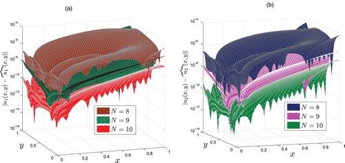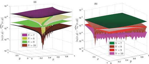The results are explained in Figure 2. We approximate the solutions at different scale level N=8,9, and 10 to analyse the amount of absolute error and noted that with the increase of scale level, the amount of absolute error decreases in a great extent. The results are visualized in Figure 3. It is worth to mention that, the absolute error at scale level N=10 is much more less than ${10}^{-8}$, which is indeed a tolerable number for such type of abstract coupled systems. The results are displayed in Figure 3.

Figure 1. Comparing approximate solutions of Example 6.1 with the exact solutions $u_1(x,y)$ and $u_2(x,y)$ at scale level N=7.

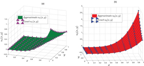
Figure 2. Comparing approximate solution with the exact solutions of Example 6.1 at fractional values of ${\eta }_1$ and ${\vartheta }_1$ at scale level N=7.

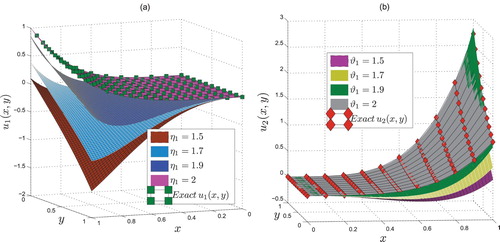
Figure 3. At different scale levels, the amount of absolute errors of Example 6.1 in $u_1(x,y)$ and $u_2(x,y)$ is noted.

Example 6.2

We consider the following coupled system of FOPDEs (46) $\begin{array}{rl}\frac{{\mathrm{\partial }}^{\left({\eta }_1\right)}}{\mathrm{\partial }{x}^{\left({\eta }_1\right)}}{u}_1(x,y)& ={\mathrm{e}}^{\left(\mathrm{\Gamma }(8-{\eta }_1)\right)}\frac{{\mathrm{\partial }}^{\left({\eta }_1-5/2\right)}}{\mathrm{\partial }{y}^{\left({\eta }_1-5/2\right)}}{u}_1(x,y)\\ & +\ln \left(\mathrm{\Gamma }\right(4-{\eta }_1\left)\right)\frac{{\mathrm{\partial }}^{\left({\eta }_1-3/2\right)}}{\mathrm{\partial }{x}^{\left({\eta }_1-3/2\right)}}{u}_2(x,y)\\ & +{\mathrm{e}}^{\left(\mathrm{\Gamma }\right({\eta }_1/2\left)\right)}\frac{{\mathrm{\partial }}^{\left({\eta }_1-7/3\right)}}{\mathrm{\partial }{y}^{\left({\eta }_1-7/3\right)}}{u}_2(x,y)\\ & +{\mathrm{e}}^{\left(\mathrm{\Gamma }\right(3\left)\right)/2}\frac{{\mathrm{\partial }}^2}{\mathrm{\partial }x\mathrm{\partial }y}{u}_2(x,y)\\ & +\mathrm{\Gamma }\left(6-\frac{3}{2}\right)\frac{{\mathrm{\partial }}^2}{\mathrm{\partial }x\mathrm{\partial }y}{u}_1(x,y)+f_1(x,y),\\ \frac{{\mathrm{\partial }}^{\left({\vartheta }_1\right)}}{\mathrm{\partial }{x}^{\left({\vartheta }_1\right)}}{u}_2(x,y)& =\sin \left(\mathrm{\Gamma }\right(8-{\vartheta }_1\left)\right)\frac{{\mathrm{\partial }}^{\left({\vartheta }_1-8/3\right)}}{\mathrm{\partial }{y}^{\left({\vartheta }_1-8/3\right)}}{u}_2(x,y)\\ & +{\mathrm{e}}^{\left(\mathrm{\Gamma }\right(7-{\vartheta }_1\left)\right)/3}\frac{{\mathrm{\partial }}^{\left({\vartheta }_1-9/4\right)}}{\mathrm{\partial }{x}^{\left({\vartheta }_1-9/4\right)}}{u}_1(x,y)\\ & +\sin \left(\mathrm{\Gamma }\right(9-{\vartheta }_1/2\left)\right)\frac{{\mathrm{\partial }}^{\left({\vartheta }_1-3/10\right)}}{\mathrm{\partial }{y}^{\left({\vartheta }_1-3/10\right)}}{u}_1(x,y)\\ & +\cos \left(\mathrm{\Gamma }\right(7-{\vartheta }_1/3\left)\right)\frac{{\mathrm{\partial }}^2}{\mathrm{\partial }x\mathrm{\partial }y}{u}_2(x,y)\\ & +\ln \left(\mathrm{\Gamma }\right(8-3/2\left)\right)\frac{{\mathrm{\partial }}^2}{\mathrm{\partial }x\mathrm{\partial }y}{u}_1(x,y)\\ & +f_2(x,y),\end{array}$(46) subject to the initial conditions (47) $\begin{array}{rl}& u_1(0,y)=u_1^{\prime }(0,y)=u_1^{″}(0,y)={\mathrm{e}}^{3y},\\ & u_2(0,y)={\mathrm{e}}^y,u_2^{\prime }(0,y)=4{\mathrm{e}}^y,u_2^{″}(0,y)=16{\mathrm{e}}^y,\\ & \mathrm{where}2<{\eta }_1\le 3,\mathrm{and}2<{\vartheta }_1\le 3.\end{array}$(47)

The source terms $f_1$ and $f_2$ are given as $\begin{array}{rl}{f}_1& =-\frac{22368075113290887286334105{\mathrm{e}}^{x+3y}}{281474976710656}\\ & -\frac{19370062200833575{\mathrm{e}}^{4x+y}}{1125899906842624},\\ f2& =\frac{277641758063497269{\mathrm{e}}^{4x+y}}{4503599627370496}\\ & -\frac{1143810618034258199{\mathrm{e}}^{x+3y}}{9007199254740992}.\end{array}$ The exact solution of the system (46(46) $\begin{array}{rl}\frac{{\mathrm{\partial }}^{\left({\eta }_1\right)}}{\mathrm{\partial }{x}^{\left({\eta }_1\right)}}{u}_1(x,y)& ={\mathrm{e}}^{\left(\mathrm{\Gamma }(8-{\eta }_1)\right)}\frac{{\mathrm{\partial }}^{\left({\eta }_1-5/2\right)}}{\mathrm{\partial }{y}^{\left({\eta }_1-5/2\right)}}{u}_1(x,y)\\ & +\ln \left(\mathrm{\Gamma }\right(4-{\eta }_1\left)\right)\frac{{\mathrm{\partial }}^{\left({\eta }_1-3/2\right)}}{\mathrm{\partial }{x}^{\left({\eta }_1-3/2\right)}}{u}_2(x,y)\\ & +{\mathrm{e}}^{\left(\mathrm{\Gamma }\right({\eta }_1/2\left)\right)}\frac{{\mathrm{\partial }}^{\left({\eta }_1-7/3\right)}}{\mathrm{\partial }{y}^{\left({\eta }_1-7/3\right)}}{u}_2(x,y)\\ & +{\mathrm{e}}^{\left(\mathrm{\Gamma }\right(3\left)\right)/2}\frac{{\mathrm{\partial }}^2}{\mathrm{\partial }x\mathrm{\partial }y}{u}_2(x,y)\\ & +\mathrm{\Gamma }\left(6-\frac{3}{2}\right)\frac{{\mathrm{\partial }}^2}{\mathrm{\partial }x\mathrm{\partial }y}{u}_1(x,y)+f_1(x,y),\\ \frac{{\mathrm{\partial }}^{\left({\vartheta }_1\right)}}{\mathrm{\partial }{x}^{\left({\vartheta }_1\right)}}{u}_2(x,y)& =\sin \left(\mathrm{\Gamma }\right(8-{\vartheta }_1\left)\right)\frac{{\mathrm{\partial }}^{\left({\vartheta }_1-8/3\right)}}{\mathrm{\partial }{y}^{\left({\vartheta }_1-8/3\right)}}{u}_2(x,y)\\ & +{\mathrm{e}}^{\left(\mathrm{\Gamma }\right(7-{\vartheta }_1\left)\right)/3}\frac{{\mathrm{\partial }}^{\left({\vartheta }_1-9/4\right)}}{\mathrm{\partial }{x}^{\left({\vartheta }_1-9/4\right)}}{u}_1(x,y)\\ & +\sin \left(\mathrm{\Gamma }\right(9-{\vartheta }_1/2\left)\right)\frac{{\mathrm{\partial }}^{\left({\vartheta }_1-3/10\right)}}{\mathrm{\partial }{y}^{\left({\vartheta }_1-3/10\right)}}{u}_1(x,y)\\ & +\cos \left(\mathrm{\Gamma }\right(7-{\vartheta }_1/3\left)\right)\frac{{\mathrm{\partial }}^2}{\mathrm{\partial }x\mathrm{\partial }y}{u}_2(x,y)\\ & +\ln \left(\mathrm{\Gamma }\right(8-3/2\left)\right)\frac{{\mathrm{\partial }}^2}{\mathrm{\partial }x\mathrm{\partial }y}{u}_1(x,y)\\ & +f_2(x,y),\end{array}$(46) ) is given as $\begin{array}{rl}{u}_1(x,y)& ={\mathrm{e}}^{x+3y},\\ u_2(x,y)& ={\mathrm{e}}^{4x+y}.\end{array}$ We examine the accuracy of our proposed method by approximating the solution of the coupled system (46(46) $\begin{array}{rl}\frac{{\mathrm{\partial }}^{\left({\eta }_1\right)}}{\mathrm{\partial }{x}^{\left({\eta }_1\right)}}{u}_1(x,y)& ={\mathrm{e}}^{\left(\mathrm{\Gamma }(8-{\eta }_1)\right)}\frac{{\mathrm{\partial }}^{\left({\eta }_1-5/2\right)}}{\mathrm{\partial }{y}^{\left({\eta }_1-5/2\right)}}{u}_1(x,y)\\ & +\ln \left(\mathrm{\Gamma }\right(4-{\eta }_1\left)\right)\frac{{\mathrm{\partial }}^{\left({\eta }_1-3/2\right)}}{\mathrm{\partial }{x}^{\left({\eta }_1-3/2\right)}}{u}_2(x,y)\\ & +{\mathrm{e}}^{\left(\mathrm{\Gamma }\right({\eta }_1/2\left)\right)}\frac{{\mathrm{\partial }}^{\left({\eta }_1-7/3\right)}}{\mathrm{\partial }{y}^{\left({\eta }_1-7/3\right)}}{u}_2(x,y)\\ & +{\mathrm{e}}^{\left(\mathrm{\Gamma }\right(3\left)\right)/2}\frac{{\mathrm{\partial }}^2}{\mathrm{\partial }x\mathrm{\partial }y}{u}_2(x,y)\\ & +\mathrm{\Gamma }\left(6-\frac{3}{2}\right)\frac{{\mathrm{\partial }}^2}{\mathrm{\partial }x\mathrm{\partial }y}{u}_1(x,y)+f_1(x,y),\\ \frac{{\mathrm{\partial }}^{\left({\vartheta }_1\right)}}{\mathrm{\partial }{x}^{\left({\vartheta }_1\right)}}{u}_2(x,y)& =\sin \left(\mathrm{\Gamma }\right(8-{\vartheta }_1\left)\right)\frac{{\mathrm{\partial }}^{\left({\vartheta }_1-8/3\right)}}{\mathrm{\partial }{y}^{\left({\vartheta }_1-8/3\right)}}{u}_2(x,y)\\ & +{\mathrm{e}}^{\left(\mathrm{\Gamma }\right(7-{\vartheta }_1\left)\right)/3}\frac{{\mathrm{\partial }}^{\left({\vartheta }_1-9/4\right)}}{\mathrm{\partial }{x}^{\left({\vartheta }_1-9/4\right)}}{u}_1(x,y)\\ & +\sin \left(\mathrm{\Gamma }\right(9-{\vartheta }_1/2\left)\right)\frac{{\mathrm{\partial }}^{\left({\vartheta }_1-3/10\right)}}{\mathrm{\partial }{y}^{\left({\vartheta }_1-3/10\right)}}{u}_1(x,y)\\ & +\cos \left(\mathrm{\Gamma }\right(7-{\vartheta }_1/3\left)\right)\frac{{\mathrm{\partial }}^2}{\mathrm{\partial }x\mathrm{\partial }y}{u}_2(x,y)\\ & +\ln \left(\mathrm{\Gamma }\right(8-3/2\left)\right)\frac{{\mathrm{\partial }}^2}{\mathrm{\partial }x\mathrm{\partial }y}{u}_1(x,y)\\ & +f_2(x,y),\end{array}$(46) )–(47(47) $\begin{array}{rl}& u_1(0,y)=u_1^{\prime }(0,y)=u_1^{″}(0,y)={\mathrm{e}}^{3y},\\ & u_2(0,y)={\mathrm{e}}^y,u_2^{\prime }(0,y)=4{\mathrm{e}}^y,u_2^{″}(0,y)=16{\mathrm{e}}^y,\\ & \mathrm{where}2<{\eta }_1\le 3,\mathrm{and}2<{\vartheta }_1\le 3.\end{array}$(47) ) at different scale level. It is noted that the approximate solution and the exact solution are in a good agreement with each other even at a very low scale level. The exact solutions $u_1(x,y)$ and $u_2(x,y)$ are compared with the approximate solutions obtained using the proposed numerical technique at scale level N=10 (see Figure 4). The accuracy of the proposed numerical technique is also investigated at various fractional values of ${\eta }_1$ and ${\vartheta }_1$, and it is observed that as both ${\eta }_1$ and ${\vartheta }_1$ approach to integer order 3, the approximate results approach to the exact solutions $u_1(x,y)$ and $u_2(x,y)$. 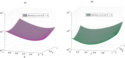The results are explained in Figure 5. We approximate the solutions at scale level N=8 to analyse the amount of absolute error and noted that, the amount of absolute error decreases to a great extent. The results are visualized in Figure 6. It is worth to mention that, the absolute error at scale level N=8 is much more less than ${10}^{-4}$, which is indeed a tolerable number for such type of abstract coupled systems. The results are displayed in Figure 6.

Figure 4. Comparing approximate solutions of Example 6.2 with the exact solutions $u_1(x,y)$ and $u_2(x,y)$ at scale level N=10.

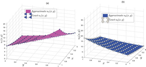
Figure 5. Comparing approximate solution with the exact solutions of Example 6.2 at fractional values of ${\eta }_1$ and ${\vartheta }_1$ at scale level N=10.

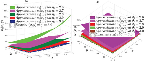
Figure 6. At scale level N=8, the amount of absolute errors of Example 6.2 in $u_1(x,y)$ and $u_2(x,y)$ is visualized.

Example 6.3

We consider the following coupled system of FOPDEs (48) $\begin{array}{rl}\frac{{\mathrm{\partial }}^{\left({\eta }_1\right)}}{\mathrm{\partial }{x}^{\left({\eta }_1\right)}}{u}_1(x,y)& =\mathrm{\Gamma }\left(3-\frac{5}{2}\right)\frac{{\mathrm{\partial }}^{1/2}}{\mathrm{\partial }{y}^{1/2}}{u}_1(x,y)\\ & +\mathrm{\Gamma }\left(4-\frac{3}{2}\right)\frac{{\mathrm{\partial }}^{1/2}}{\mathrm{\partial }{x}^{1/2}}{u}_2(x,y)\\ & +\mathrm{\Gamma }\left(3-\frac{5}{2}\right)\frac{{\mathrm{\partial }}^{3/2}}{\mathrm{\partial }{y}^{3/2}}{u}_2(x,y)\\ & +\mathrm{\Gamma }\left(3\right)\frac{{\mathrm{\partial }}^2}{\mathrm{\partial }x\mathrm{\partial }y}{u}_2(x,y)\\ & +\mathrm{\Gamma }\left(6-\frac{3}{2}\right)\frac{{\mathrm{\partial }}^2}{\mathrm{\partial }x\mathrm{\partial }y}{u}_1(x,y)+f_1(x,y),\\ \frac{{\mathrm{\partial }}^{\left({\vartheta }_1\right)}}{\mathrm{\partial }{x}^{\left({\vartheta }_1\right)}}{u}_2(x,y)& =\mathrm{\Gamma }\left(8-\frac{5}{2}\right)\frac{{\mathrm{\partial }}^{3/2}}{\mathrm{\partial }{y}^{3/2}}{u}_2(x,y)\\ & +\mathrm{\Gamma }\left(7-\frac{3}{2}\right)\frac{{\mathrm{\partial }}^{1/2}}{\mathrm{\partial }{x}^{1/2}}{u}_1(x,y)\\ & +\mathrm{\Gamma }\left(9-\frac{5}{4}\right)\frac{{\mathrm{\partial }}^{3/10}}{\mathrm{\partial }{y}^{3/10}}{u}_1(x,y)\\ & +\mathrm{\Gamma }\left(7-\frac{8}{9}\right)\frac{{\mathrm{\partial }}^2}{\mathrm{\partial }x\mathrm{\partial }y}{u}_2(x,y)\\ & +\mathrm{\Gamma }\left(8-\frac{3}{2}\right)\frac{{\mathrm{\partial }}^2}{\mathrm{\partial }x\mathrm{\partial }y}{u}_1(x,y)+f_2(x,y),\end{array}$(48) subject to the initial conditions (49) $\begin{array}{rl}& u_1(0,y)=0,u_1^{\prime }(0,y)=\frac{1384633456860719\cos \left(y\right)}{562949953421312},\\ & u_2(0,y)=0,u_2^{\prime }(0,y)=\frac{3039611811401035\cos \left(y\right)}{2251799813685248},\\ & \mathrm{where}1<{\eta }_1\le 2,\mathrm{and}1<{\vartheta }_1\le 2.\end{array}$(49)

The source terms $f_1$ and $f_2$ are given as $\begin{array}{rl}{f}_1& =\frac{4961133318983242280583421095261\cos \left(x\right)\sin \left(y\right)}{158456325028528675187087900672}\\ & -\frac{1137349955723420952606451170995\cos \left(x\right)\cos \left(y\right)}{633825300114114700748351602688}\\ & -\frac{679873159350975344197965671591\cos \left(y\right)\sin \left(x\right)}{10141204801825835211973625643008}\\ & +\frac{11052729263717111494726278938277\sin \left(x\right)\sin \left(y\right)}{2535301200456458802993406410752},\\ f2& =\frac{71629770435166584613696367360639\cos \left(x\right)\sin \left(y\right)}{79228162514264337593543950336}\\ & -\frac{10200028470910811599972491009437\cos \left(x\right)\cos \left(y\right)}{79228162514264337593543950336}\\ & -\frac{2361545807795474570465951640319695\cos \left(y\right)\sin \left(x\right)}{316912650057057350374175801344}\\ u_1(x,y)& =\sin \left(x\right)\cos \left(y\right){\mathrm{e}}^{0.9},\\ u_2(x,y)& =\sin \left(x\right)\cos \left(y\right){\mathrm{e}}^{0.3}.\end{array}$ We examine the accuracy of our proposed method by approximating the solution of the coupled system (48(48) $\begin{array}{rl}\frac{{\mathrm{\partial }}^{\left({\eta }_1\right)}}{\mathrm{\partial }{x}^{\left({\eta }_1\right)}}{u}_1(x,y)& =\mathrm{\Gamma }\left(3-\frac{5}{2}\right)\frac{{\mathrm{\partial }}^{1/2}}{\mathrm{\partial }{y}^{1/2}}{u}_1(x,y)\\ & +\mathrm{\Gamma }\left(4-\frac{3}{2}\right)\frac{{\mathrm{\partial }}^{1/2}}{\mathrm{\partial }{x}^{1/2}}{u}_2(x,y)\\ & +\mathrm{\Gamma }\left(3-\frac{5}{2}\right)\frac{{\mathrm{\partial }}^{3/2}}{\mathrm{\partial }{y}^{3/2}}{u}_2(x,y)\\ & +\mathrm{\Gamma }\left(3\right)\frac{{\mathrm{\partial }}^2}{\mathrm{\partial }x\mathrm{\partial }y}{u}_2(x,y)\\ & +\mathrm{\Gamma }\left(6-\frac{3}{2}\right)\frac{{\mathrm{\partial }}^2}{\mathrm{\partial }x\mathrm{\partial }y}{u}_1(x,y)+f_1(x,y),\\ \frac{{\mathrm{\partial }}^{\left({\vartheta }_1\right)}}{\mathrm{\partial }{x}^{\left({\vartheta }_1\right)}}{u}_2(x,y)& =\mathrm{\Gamma }\left(8-\frac{5}{2}\right)\frac{{\mathrm{\partial }}^{3/2}}{\mathrm{\partial }{y}^{3/2}}{u}_2(x,y)\\ & +\mathrm{\Gamma }\left(7-\frac{3}{2}\right)\frac{{\mathrm{\partial }}^{1/2}}{\mathrm{\partial }{x}^{1/2}}{u}_1(x,y)\\ & +\mathrm{\Gamma }\left(9-\frac{5}{4}\right)\frac{{\mathrm{\partial }}^{3/10}}{\mathrm{\partial }{y}^{3/10}}{u}_1(x,y)\\ & +\mathrm{\Gamma }\left(7-\frac{8}{9}\right)\frac{{\mathrm{\partial }}^2}{\mathrm{\partial }x\mathrm{\partial }y}{u}_2(x,y)\\ & +\mathrm{\Gamma }\left(8-\frac{3}{2}\right)\frac{{\mathrm{\partial }}^2}{\mathrm{\partial }x\mathrm{\partial }y}{u}_1(x,y)+f_2(x,y),\end{array}$(48) )–(49(49) $\begin{array}{rl}& u_1(0,y)=0,u_1^{\prime }(0,y)=\frac{1384633456860719\cos \left(y\right)}{562949953421312},\\ & u_2(0,y)=0,u_2^{\prime }(0,y)=\frac{3039611811401035\cos \left(y\right)}{2251799813685248},\\ & \mathrm{where}1<{\eta }_1\le 2,\mathrm{and}1<{\vartheta }_1\le 2.\end{array}$(49) ) at different scale level. It is noted that the approximate solution and the exact solution are in a good agreement with each other even at a very low scale level. The exact solutions $u_1(x,y)$ and $u_2(x,y)$ are compared with the approximate solutions obtained using the proposed numerical technique at scale level N=7 (see Figure 7). The accuracy of the proposed numerical technique is also investigated at various fractional values of ${\eta }_1$ and ${\vartheta }_1$, and it is observed that as both ${\eta }_1$ and ${\vartheta }_1$ approach to integer order 2, the approximate results approach to the exact solutions $u_1(x,y)$ and $u_2(x,y)$. The results are explained in Figure 8. We approximate the solutions at different scale level N=7,8,9, and 10 to analyse the amount of absolute error and noted that with the increase of scale level, the amount of absolute error decreases in a great extent. The results are visualized in Figure 9. It is worth to mention that, the absolute error at scale level N=10 is much more less than ${10}^{-4}$, which is indeed a tolerable number for such type of abstract coupled systems. The results are displayed in Figure 9.

Figure 7. Comparing approximate solutions of Example 6.3 with the exact solutions $u_1(x,y)$ and $u_2(x,y)$ at scale level N=7.

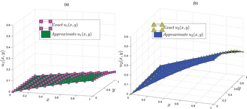
Figure 8. Comparing approximate solution with the exact solutions of Example 6.3 at fractional values of ${\eta }_1$ and ${\vartheta }_1$ at scale level N=7.

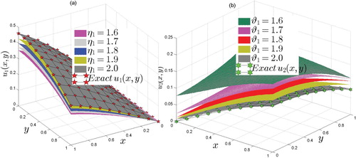
Figure 9. At different scale levels, the amount of absolute errors of Example 6.3 in $u_1(x,y)$ and $u_2(x,y)$ is visualized.

7. Conclusion

Our main objective in this article was the development of the new numerical method for finding the approximate solution of generalized FOCSs with mixed partial derivative terms of fractional order. The objective has been achieved by developing a method based on the operational matrices of Riemann-Liouville fractional integrals and Caputo fractional derivatives of SLPs. The experimental results show that the results are in a good agreement with the exact solution with a low number of approximating terms.

The proposed method has the ability to simplify the task of finding the solution of generalized FOCSs by transforming them into system of equations which are algebraic in nature. One salient aspect of our research is the development of a new fractional operational matrix for mixed partial derivatives in the sense of Caputo. This theory can also be applied to solve the problems numerically existing in fluid dynamics and to many other linear and nonlinear problems of fractional order.

Disclosure statement

No potential conflict of interest was reported by the authors.

ORCID

Imran Talib http://orcid.org/0000-0003-0115-4506

Cemil Tunc http://orcid.org/0000-0003-2909-8753

Zulfiqar Ahmad Noor http://orcid.org/0000-0001-7232-6112

References

- He JH. Some applications of nonlinear fractional differential equations and their approximations. Bull Sci Technol. 1999;15(2):86–90.
- He JH. Nonlinear oscillation with fractional derivative and its applications. In: International Conference on Vibrating Engineering'98, Dalian, China. 1998. p. 288–291.
- Freed AD, Diethelm K. Fractional calculus in biomechanics: a 3D viscoelastic model using regularized fractional derivative kernels with application to the human calcaneal fat pad. Biomechan Model Mechanobiol. 2006;5(4):203–215. doi: 10.1007/s10237-005-0011-0
- Magin RL. Fractional calculus in bioengineering. Crit Rev Biomed Eng. 2004;32(1):1–104. doi: 10.1615/CritRevBiomedEng.v32.10
- Chow TS. Fractional dynamics of interfaces between soft-nanoparticles and rough substrates. Phys Lett A. 2005;342:148–155. doi: 10.1016/j.physleta.2005.05.045
- Metzler R, Klafter J. The restaurant at the end of the random walk: Recent developments in the description of anomalous transport by fractional dynamics. J Phys A. 2004;37:161–208. doi: 10.1088/0305-4470/37/31/R01
- Wang JR, Zhou Y. A class of fractional evolution equations and optimal controls. Nonlinear Anal RWA. 2011;12:262–272. doi: 10.1016/j.nonrwa.2010.06.013
- Ervin VJ, Roop JP. Variational formulation for the stationary fractional advection dispersion equation. Numer Methods Partial Differ Equ. 2005;22:558–576. doi: 10.1002/num.20112
- Rawashdeh EA. Numerical solution of fractional integro-differential equations by collocation method. Appl Math Comput. 2006;176:1–6.
- Momani S, Shawagfeh NT. Decomposition method for solving fractional Riccati differential equations. Appl Math Comput. 2006;182:1083–1092.
- Gejji VD, Jafari H. Solving a multi-order fractional differential equation. Appl Math Comput. 2007;189:541–548.
- Saadatmandi A, Dehghan M. A new operational matrix for solving fractional-order differential equations. Comput Math Appl. 2010;59:1326–1336. doi: 10.1016/j.camwa.2009.07.006
- Talib I, Belgacem FBM, Asif NA, et al. On mixed derivatives type high dimensional multi-term fractional partial differential equations approximate solutions. Amer Inst Phys. 2017. doi:10.1063/1.4972616
- Khalil H, Khan RA. A new method based on Legendre polynomials for solution of system of fractional order partial differential equations. Int J Comput Math. 2014;91(12):2554–2567. doi: 10.1080/00207160.2014.880781
- Bhrawy AH, Alofi AS. The operational matrix of fractional integration for shifted Chebyshev polynomials. Appl Math Lett. 2013;26(1):25–31. doi: 10.1016/j.aml.2012.01.027
- Doha EH, Bhrawy AH, Ezz-Eldien SS. A new Jacobi operational matrix: an application for solving fractional differential equations. Appl Math Model. 2012;36(10):4931–4943. doi: 10.1016/j.apm.2011.12.031
- Saadatmandi A. Bernstein operational matrix of fractional derivatives and its applications. Appl Math Model. 2014;38(4):1365–1372. doi: 10.1016/j.apm.2013.08.007
- Maleknejad K, Hashemizadeh E, Basirat B. Computational method based on Bernstein operational matrices for nonlinear Volterra–Fredholm–Hammerstein integral equations. Commun Nonlinear Sci Numer Simul. 2012;17(1):52–61. doi: 10.1016/j.cnsns.2011.04.023
- Bhrawy AH, Doha EH, Baleanu D, et al. A spectral tau algorithm based on Jacobi operational matrix for numerical solution of time fractional diffusion-wave equations. J Comput Phys. 2015;293:142–156. doi: 10.1016/j.jcp.2014.03.039
- Erjaee GH, Akrami MH, Atabakzadeh MH. The operational matrix of fractional integration for shifted Legendre polynomials. Iranian J Sci Technol (Sciences). 2013;37(4):439–444.
- Ahmed HF. A numerical technique for solving multi-dimensional fractional optimal control problems. J Taibah Univ Sci. 2018;12(5):494–505. DOI:10.1080/16583655.2018.1491690
- Saadatmandi A, Razzaghi M, Dehghan M. Hartley series approximations for the parabolic equations. Int J Comput Math. 2006;82:1149–1156. doi: 10.1080/00207160500113066
- Saadatmandi A, Dehghan M. A Tau method for the one-dimensional parabolic inverse problem subject to temperature overspecification. Comput Math Appl. 2006;52:933–940. doi: 10.1016/j.camwa.2006.04.017
- Barenblatt GI, Zheltov PIu, Kochina IN. Basic concepts in the theory of seepage of homogeneous liquids in fissured rocks (strata). Prikald Mat Mehk. 1960;24:852–864.
- Coleman BD, Noll W. An approximation theorem for functionals, with application in continuum mechanics. Arch Ration Mech Anal. 1960;6:355–370. doi: 10.1007/BF00276168
- Podlubny I. Fractional differential equations: an introduction to fractional derivatives, fractional differential equations, to methods of their solutions and some of their applications. New York: Academic Press; 1998.
- Caputo M. Linear models of dissipation whose Q is almost frequency independent. Part II. Geophys J Int. 1967;13:529–539. doi: 10.1111/j.1365-246X.1967.tb02303.x
- Kilbas AA, Srivastava HM, Trujillo JJ. Theory and applications of fractional differential equations. San Diego (CA): Elsevier; 2006.
- Villiers JD. Mathematics of approximation. Beijing: Springer, Atlantis Press; 2012.