Alpha power inverse Weibull distribution with reliability application

Abstract

In this paper, we use the method of the alpha power transformation to introduce a new generalized alpha power inverse Weibull (APIW) distribution. Its characterization and statistical properties are obtained, such as reliability, moments, entropy and order statistics. Moreover, the estimation of the APIW parameters is discussed by using maximum likelihood estimation method. Finally, the application of the proposed new distribution to a real data representing the waiting time before customer service in the bank is given and its goodness-of-fit is demonstrated. In addition, comparisons to other models are carried out to illustrate the flexibility of the proposed model.

Keywords:

• Alpha power transformation
• inverse Weibull distribution
• reliability
• moments
• maximum likelihood estimation
• simulation

1. Introduction

The inverse Weibull (IW) distribution plays an important role in many applications, including the dynamic components of diesel engine and several data set such as the times to breakdown of an insulating fluid subject to the action of a constant tension, see Nelson [1]. Inverse Weibull distribution with parameters λ and β with cumulative distribution function and the probability density function of a random variable X are respectively given by (1) $\begin{array}{r}F\left(x\right)={\mathrm{e}}^{-\lambda x^{-\text{β}}},x\ge 0,\lambda >0,\text{β}>0,\end{array}$(1) and (2) $\begin{array}{r}f\left(x\right)=\lambda \text{β}{x}^{-(\text{β}+1)}{\mathrm{e}}^{-\lambda x^{-\text{β}}},x\ge 0,\lambda >0,\text{β}>0.\end{array}$(2)

A lot of work has been done on inverse Weibull distribution, for example, Calabria and Pulcini [2] have studied the maximum likelihood and least square estimation of the inverse Weibull distribution. Calabria and Pulcini [3] have studied Bayes 2-sample prediction for inverse Weibull distribution. Maswadah in [4] has the fitted inverse Weibull distribution to the flood data. Some important theoretical analysis of the inverse Weibull distribution was studied by Khan et al. [5].

In the recent past, many generalizations of inverse Weibull distribution have been studied by authors such as mixture of two inverse Weibull distributions by Sultan et al. [6], the generalized inverse Weibull distribution by De Gusmao et al. [7], modified inverse Weibull distribution by Khan and King [8], beta inverse Weibull by Hanook et al. [9], gamma inverse Weibull distribution by Pararai et al. [10], Kumaraswamy modified inverse Weibull distribution by Aryal and Elbatal [11], reflected generalized beta inverse Weibull distribution by Elbatal et al. [12] and Marshall–Olkin extended inverse Weibull distribution by Okasha et al. [13].

On the other hand, Mahdavi and Kundu [14] proposed a transformation of the baseline (CDF) by adding a new parameter to obtain a family of distributions. The proposed method is called alpha power transformation (APT). If $F\left(x\right)$ be a cumulative density function of any distribution, then the $G_{{}_{APT}}\left(x\right)$ is cumulative density function distribution (3) $\begin{array}{rl}{G}_{{}_{APT}}\left(x\right)& =\left\{\begin{array}{ll}\frac{{\alpha }^{F\left(x\right)}-1}{\alpha -1},& \alpha >0,\alpha \ne 1\\ F\left(x\right),& \alpha =1,\end{array}\right.\end{array}$(3) and the corresponding probability density function (PDF) as (4) $\begin{array}{rl}{g}_{{}_{APT}}\left(x\right)& =\left\{\begin{array}{ll}\frac{\log \left(\alpha \right)}{\alpha -1}f\left(x\right){\alpha }^{F\left(x\right)},& \alpha >0,\alpha \ne 1\\ f\left(x\right),& \alpha =1.\end{array}\right.\end{array}$(4)

The main aim of this paper is to propose and study a new distribution model called APIW distribution based on the method of APT. The rest of the paper is organized as follows. In Section 2, we define our proposed model and its special cases are presented. In Section 3, its reliability analysis is given. In Section 4, its statistical properties are given. The parameters of this distribution are estimated by the maximum likelihood estimation (MLE) method in Section 5. Finally, the proposed model is applied on real data and the results are given in Section 6.

2. New model

In this section, we will give the alpha power inverse Weibull (APIW) distribution and some of its submodels.

2.1. APIW specification

Let $\mathrm{\Theta }=(\alpha ,\lambda ,\text{β})$ and by substitution the cumulative function of inverse Weibull given by (1(1) $\begin{array}{r}F\left(x\right)={\mathrm{e}}^{-\lambda x^{-\text{β}}},x\ge 0,\lambda >0,\text{β}>0,\end{array}$(1) ) in alpha power is given by (3(3) $\begin{array}{rl}{G}_{{}_{APT}}\left(x\right)& =\left\{\begin{array}{ll}\frac{{\alpha }^{F\left(x\right)}-1}{\alpha -1},& \alpha >0,\alpha \ne 1\\ F\left(x\right),& \alpha =1,\end{array}\right.\end{array}$(3) ) we get a new distribution denoted as APIW $(x,\mathrm{\Theta })$ distribution with CDF given by (5) $\begin{array}{rl}{G}_{{}_{APIW}}\left(x\right)& =\left\{\begin{array}{ll}\frac{{\alpha }^{{\mathrm{e}}^{-\lambda x^{-\text{β}}}}-1}{\alpha -1},& \alpha >0,\alpha \ne 1\\ {\mathrm{e}}^{-\lambda x^{-\text{β}}},& \alpha =1,\end{array}\right.\end{array}$(5) its corresponding probability density function (PDF) is given by (6) $\begin{array}{rl}{g}_{{}_{APIW}}\left(x\right)& =\left\{\begin{array}{l}\frac{\log \left(\alpha \right)}{\alpha -1}\lambda \text{β}{x}^{-(\text{β}+1)}{\mathrm{e}}^{-\lambda x^{-\text{β}}}{\alpha }^{{\mathrm{e}}^{-\lambda x^{-\text{β}}}},\\ \alpha >0,\alpha \ne 1\\ \lambda \text{β}{x}^{-(\text{β}+1)}{\mathrm{e}}^{-\lambda x^{-\text{β}}},\alpha =1.\end{array}\right.\end{array}$(6)

By using the Taylor's series expansion of the function ${\alpha }^{{\mathrm{e}}^{-\lambda t^{-\text{β}}}}$, we can rewrite the PDF when $\alpha >0,\alpha \ne 1$ as follows: (7) $\begin{array}{rl}{g}_{{}_{APIW}}\left(x\right)& =\frac{1}{\alpha -1}\sum _{j=0}^{\mathrm{\infty }}\frac{(\log (\alpha ){)}^{j+1}}{j!}\lambda \text{β}{x}^{-(\text{β}+1)}{\mathrm{e}}^{-\lambda (j+1)x^{-\text{β}}}.\end{array}$(7)

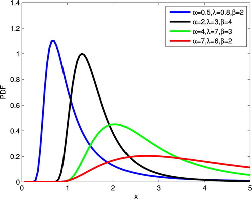
Figure 1 gives the graphical representation of PDF for different values of α, λ and β.

Figure 1. Plot of the PDF of the APIW distribution.

2.2. APIW submodels

Equation (5(5) $\begin{array}{rl}{G}_{{}_{APIW}}\left(x\right)& =\left\{\begin{array}{ll}\frac{{\alpha }^{{\mathrm{e}}^{-\lambda x^{-\text{β}}}}-1}{\alpha -1},& \alpha >0,\alpha \ne 1\\ {\mathrm{e}}^{-\lambda x^{-\text{β}}},& \alpha =1,\end{array}\right.\end{array}$(5) ) of the APIW distribution includes the following well-known distributions as submodels.

1. If $\lambda =1$, then (5(5) $\begin{array}{rl}{G}_{{}_{APIW}}\left(x\right)& =\left\{\begin{array}{ll}\frac{{\alpha }^{{\mathrm{e}}^{-\lambda x^{-\text{β}}}}-1}{\alpha -1},& \alpha >0,\alpha \ne 1\\ {\mathrm{e}}^{-\lambda x^{-\text{β}}},& \alpha =1,\end{array}\right.\end{array}$(5) ) reduces to alpha power Fréchet (APF) distribution.

2. If $\text{β}=2$, then (5(5) $\begin{array}{rl}{G}_{{}_{APIW}}\left(x\right)& =\left\{\begin{array}{ll}\frac{{\alpha }^{{\mathrm{e}}^{-\lambda x^{-\text{β}}}}-1}{\alpha -1},& \alpha >0,\alpha \ne 1\\ {\mathrm{e}}^{-\lambda x^{-\text{β}}},& \alpha =1,\end{array}\right.\end{array}$(5) ) reduces to alpha power inverse Rayleigh (APIR) distribution.

3. If $\text{β}=1$, then (5(5) $\begin{array}{rl}{G}_{{}_{APIW}}\left(x\right)& =\left\{\begin{array}{ll}\frac{{\alpha }^{{\mathrm{e}}^{-\lambda x^{-\text{β}}}}-1}{\alpha -1},& \alpha >0,\alpha \ne 1\\ {\mathrm{e}}^{-\lambda x^{-\text{β}}},& \alpha =1,\end{array}\right.\end{array}$(5) ) reduces to alpha power inverse exponential (APIE) distribution.

4. If $\alpha =1$, then (5(5) $\begin{array}{rl}{G}_{{}_{APIW}}\left(x\right)& =\left\{\begin{array}{ll}\frac{{\alpha }^{{\mathrm{e}}^{-\lambda x^{-\text{β}}}}-1}{\alpha -1},& \alpha >0,\alpha \ne 1\\ {\mathrm{e}}^{-\lambda x^{-\text{β}}},& \alpha =1,\end{array}\right.\end{array}$(5) ) reduces to inverse Weibull (IW) distribution.

5. If $\alpha =1$ and $\lambda =1$, then (5(5) $\begin{array}{rl}{G}_{{}_{APIW}}\left(x\right)& =\left\{\begin{array}{ll}\frac{{\alpha }^{{\mathrm{e}}^{-\lambda x^{-\text{β}}}}-1}{\alpha -1},& \alpha >0,\alpha \ne 1\\ {\mathrm{e}}^{-\lambda x^{-\text{β}}},& \alpha =1,\end{array}\right.\end{array}$(5) ) reduces to Fréchet (F) distribution.

6. If $\alpha =1$ and $\text{β}=2$, then (5(5) $\begin{array}{rl}{G}_{{}_{APIW}}\left(x\right)& =\left\{\begin{array}{ll}\frac{{\alpha }^{{\mathrm{e}}^{-\lambda x^{-\text{β}}}}-1}{\alpha -1},& \alpha >0,\alpha \ne 1\\ {\mathrm{e}}^{-\lambda x^{-\text{β}}},& \alpha =1,\end{array}\right.\end{array}$(5) ) reduces to inverse Rayleigh (IR) distribution.

7. If $\alpha =1$ and $\text{β}=1$, then (5(5) $\begin{array}{rl}{G}_{{}_{APIW}}\left(x\right)& =\left\{\begin{array}{ll}\frac{{\alpha }^{{\mathrm{e}}^{-\lambda x^{-\text{β}}}}-1}{\alpha -1},& \alpha >0,\alpha \ne 1\\ {\mathrm{e}}^{-\lambda x^{-\text{β}}},& \alpha =1,\end{array}\right.\end{array}$(5) ) reduces to inverse exponential (IE) distribution.

3. Reliability analysis

The reliability function (survival function) of APIW distribution is given by (8) $\begin{array}{rl}{R}_{{}_{APIW}}\left(t\right)& =\left\{\begin{array}{ll}\frac{\alpha }{\alpha -1}(1-{\alpha }^{{\mathrm{e}}^{-\lambda t^{-\text{β}}}-1}),& \alpha >0,\alpha \ne 1\\ 1-{\mathrm{e}}^{-\lambda t^{-\text{β}}},& \alpha =1.\end{array}\right.\end{array}$(8)

3.1. Hazard rate function

The hazard rate ( HR) function (failure rate) of a lifetime random variable X with APIW distribution is given by (9) $\begin{array}{rl}{h}_{{}_{APIW}}\left(t\right)& =\left\{\begin{array}{l}\log \left(\alpha \right)\lambda \text{β}{t}^{-(\text{β}+1)}{\mathrm{e}}^{-\lambda t^{-\text{β}}}\frac{{\alpha }^{{\mathrm{e}}^{-\lambda t^{-\text{β}}}-1}}{1-{\alpha }^{{\mathrm{e}}^{-\lambda t^{-\text{β}}}-1}},\alpha >0,\alpha \ne 1\\ \frac{\lambda \text{β}{t}^{-(\text{β}+1)}{\mathrm{e}}^{-\lambda t^{-\text{β}}}}{1-{\mathrm{e}}^{-\lambda t^{-\text{β}}}},\alpha =1.\end{array}\right.\end{array}$(9)

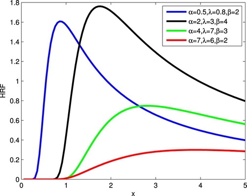
Figure 2 gives the graphical representation of HRF for different values of α, λ and β.

Figure 2. Plot of the HRF of the APIW distribution.

3.2. Reversed hazard rate function

The reversed hazard rate (RHR) function of a lifetime random variable X with APIW distribution is given by (10) $\begin{array}{rl}{r}_{{}_{APIW}}\left(t\right)& =\left\{\begin{array}{l}\log \left(\alpha \right)\lambda \text{β}{t}^{-(\text{β}+1)}{\mathrm{e}}^{-\lambda t^{-\text{β}}}\frac{{\alpha }^{{\mathrm{e}}^{-\lambda t^{-\text{β}}}}}{{\alpha }^{{\mathrm{e}}^{-\lambda t^{-\text{β}}}}-1},\alpha >0,\alpha \ne 1\\ \lambda \text{β}{t}^{-(\text{β}+1)},\alpha =1.\end{array}\right.\end{array}$(1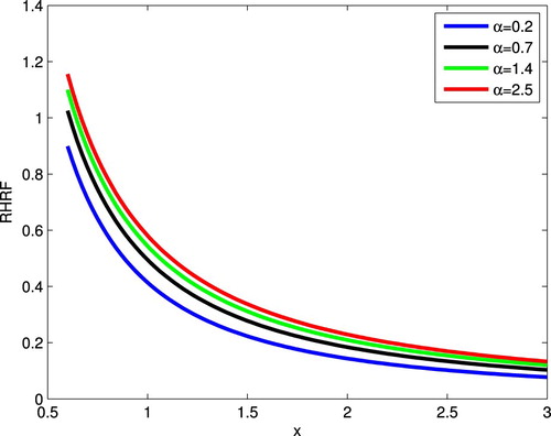0) Figure 3 gives graphical representations of RHRF for different values of α.

Figure 3. Plot of the RHRF of the APIW distribution where $\lambda =0.3,\text{β}=2.$

3.3. Mean residual life

The mean residual life (MRL) function describes the aging process, so it is very important in reliability and survival analysis. The MRL function of a lifetime random variable X is given by $\begin{array}{rl}\mu \left(t\right)& =\frac{1}{R\left(t\right)}{\int }_t^{\mathrm{\infty }}xg\left(x\right)\mathrm{d}x-t,t>0.\end{array}$

Theorem 3.1

The MRL function of a lifetime random variable X with APIW is given by (11) $\begin{array}{rl}\mu \left(t\right)& =\frac{1}{R\left(t\right)}\frac{{\lambda }^{1/\text{β}}}{\alpha -1}\sum _{j=0}^{\mathrm{\infty }}\frac{(\log (\alpha ){)}^{j+1}}{(j+1)!}(j+1{)}^{1/\text{β}}\\ & \times \gamma \left(1-\frac{1}{\text{β}},\lambda (j+1)t^{-\text{β}}\right)-t,\text{β}>1.\end{array}$(11)

Proof.

From definition of MRL, we get $\begin{array}{rl}\mu \left(t\right)& =\frac{1}{R\left(t\right)}{\int }_t^{\mathrm{\infty }}xg\left(x\right)\mathrm{d}x-t\\ & =\frac{1}{R\left(t\right)}\frac{1}{\alpha -1}\sum _{j=0}^{\mathrm{\infty }}\frac{(\log (\alpha ){)}^{j+1}}{j!}\\ & \times {\int }_t^{\mathrm{\infty }}x.\lambda \text{β}{x}^{-(\text{β}+1)}{\mathrm{e}}^{-\lambda (j+1)x^{-\text{β}}}\mathrm{d}x-t,\end{array}$ put $y=\lambda (j+1)x^{-\text{β}}$, thus $\begin{array}{rl}\mu \left(t\right)& =\frac{1}{R\left(t\right)}\frac{{\lambda }^{1/\text{β}}}{\alpha -1}\sum _{j=0}^{\mathrm{\infty }}\left((\log (\alpha ){)}^{j+1}/(j+1)!\right)(j+1{)}^{1/\text{β}}\\ & \times \gamma \left(1-\frac{1}{\text{β}},\alpha (j+1)t^{-\text{β}}\right)-t,\end{array}$ where $\gamma (c,t)={\int }_0^t{x}^{c-1}{\mathrm{e}}^{-x}\mathrm{d}x$, c>0.

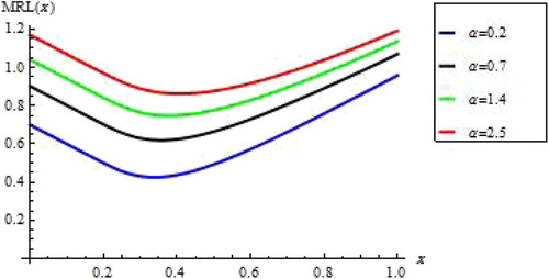
Figure 4 gives graphical representations of MRL for different values of α.

Figure 4. Plot of the MRL of the APIW distribution where $\lambda =0.3,\text{β}=2.$

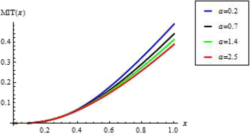
3.4. Mean inactivity time

The mean inactivity time (MIT) function is a recognized reliability measure which has applications such as forensic science, reliability theory and survival analysis. The MIT function of a lifetime random variable X is given by $\begin{array}{rl}m\left(t\right)& =t-\frac{1}{G\left(t\right)}{\int }_0^{t}xg\left(x\right)\mathrm{d}x,t>0.\end{array}$

Theorem 3.2

The MIT function of a lifetime random variable X with APIW is given by (12) $\begin{array}{rl}m\left(t\right)& =t-\frac{1}{G\left(t\right)}\frac{{\lambda }^{1/\text{β}}}{\alpha -1}\sum _{j=0}^{\mathrm{\infty }}\frac{(\log (\alpha ){)}^{j+1}}{(j+1)!}(j+1{)}^{1/\text{β}}\\ & \times \mathrm{\Gamma }\left(1-\frac{1}{\text{β}},\lambda (j+1)t^{-\text{β}}\right),\text{β}>1.\end{array}$(12)

Proof.

Using the proof of MRL and the relation $\mathrm{\Gamma }(c,t)={\int }_t^{\mathrm{\infty }}{x}^{c-1}{\mathrm{e}}^{-x}\mathrm{d}x$, c>0,

we get the above result.

Figure 5 gives graphical representations of MIT for different values of α.

Figure 5. Plot of the MIT of the APIW distribution where $\lambda =0.3,\text{β}=2.$

3.5. Strong mean inactivity time

The strong mean inactivity time (SMIT) is a new reliability function which was proposed by Kayid and Izadkhah [15]. The SMIT function of a lifetime random variable X is given by $\begin{array}{rl}M\left(t\right)& =\frac{1}{G\left(t\right)}{\int }_0^{t}2xG\left(x\right)\mathrm{d}x\\ & =t^2-\frac{1}{G\left(t\right)}{\int }_0^t{x}^{2}g\left(x\right)\mathrm{d}x,t>0.\end{array}$

Theorem 3.3

The SMIT function of a lifetime random variable X with APIW is given by (13) $\begin{array}{rl}M\left(t\right)& =t^2-\frac{1}{G\left(t\right)}\frac{{\lambda }^{2/\text{β}}}{\alpha -1}\sum _{j=0}^{\mathrm{\infty }}\frac{(\log (\alpha ){)}^{j+1}}{(j+1)!}(j+1{)}^{2/\text{β}}\\ & \times \mathrm{\Gamma }\left(1-\frac{2}{\text{β}},\lambda (j+1)t^{-\text{β}}\right),\text{β}>2.\end{array}$(13)

Proof.

Using the proof of MRL and the relation $\mathrm{\Gamma }(c,t)={\int }_t^{\mathrm{\infty }}{x}^{c-1}{\mathrm{e}}^{-x}\mathrm{d}x$, c>0,

we get the above result.

Figure 6 gives graphical representations of SMIT for different values of α.

Figure 6. Plot of the SMIT of the APIW distribution where $\lambda =0.3,\text{β}=2.$

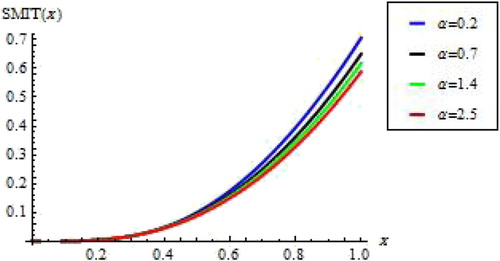
Table 1 gives the values of HR, MRL, RHR and MIT(SMIT) for the selected values of $\lambda =0.7$, $\text{β}=1.8$ and t=0.6 and for different values of the parameter α. One can observe that the values of HR are decreasing and values of MRL are increasing and the same for RHR and MIT (SMIT).

Table 1. Some reliability of APIW for selected values of λ=0.7 and β=1.8 at t=0.6.

Parameter α	HR	MRL	RHR	MIT	SMIT
α=0.2	1.99054	0.80185	4.5683	0.11868	0.122262
α=0.7	1.27053	1.15554	5.1061	0.11394	0.117785
α=1.4	0.95422	1.39307	5.4214	0.11134	0.115314
α=2.5	0.73545	1.61125	5.6947	0.10917	0.113254

3.6. Stress–strength reliability

In the reliability, the stress–strength (supply–demand) model describes the life of a component which has a random strength X that is subjected to a random stress Z. The component fails at the instant that the stress applied to it exceeds the strength, and the component will function satisfactorily whenever X>Z. Hence, $R=Pr(X>Z)$ is a measure of component reliability. It has many applications in several areas of engineering and science.

We now derive the reliability R when X and Z have independent APIW (${\alpha }_1,{\lambda }_1,\text{β}$) and APIW (${\alpha }_2,{\lambda }_2,\text{β}$) distributions with the same shape parameter β. The PDF of X and the CDF of Z can be expressed from respectively as $\begin{array}{rl}{g}_1\left(t\right)& =\frac{\log \left({\alpha }_1\right)}{{\alpha }_1-1}{\lambda }_1\text{β}{t}^{-(\text{β}+1)}{\mathrm{e}}^{-{\lambda }_1{t}^{-\text{β}}}{\alpha }_1^{{\mathrm{e}}^{-{\lambda }_1{t}^{-\text{β}}}}\end{array}$ and $\begin{array}{rl}{G}_2\left(t\right)& =\frac{{\alpha }_2^{{\mathrm{e}}^{-{\lambda }_2{t}^{-\text{β}}}}-1}{{\alpha }_2-1}.\end{array}$ We have $\begin{array}{rl}R& ={\int }_0^{\mathrm{\infty }}{g}_1\left(t\right)G_2\left(t\right)\mathrm{d}t=\frac{{\lambda }_1\text{β}\log \left({\alpha }_1\right)}{({\alpha }_1-1)({\alpha }_2-1)}\\ & \times {\int }_0^{\mathrm{\infty }}{t}^{-(\text{β}+1)}{\mathrm{e}}^{-{\lambda }_1{t}^{-\text{β}}}{\alpha }_1^{{\mathrm{e}}^{-{\lambda }_1{t}^{-\text{β}}}}({\alpha }_2^{{\mathrm{e}}^{-{\lambda }_2{t}^{-\text{β}}}}-1)\mathrm{d}t\\ & =\frac{{\lambda }_1\text{β}\log \left({\alpha }_1\right)}{({\alpha }_1-1)({\alpha }_2-1)}\\ & \times {\int }_0^{\mathrm{\infty }}{t}^{-(\text{β}+1)}{\mathrm{e}}^{-{\lambda }_1{t}^{-\text{β}}}{\alpha }_1^{{\mathrm{e}}^{-{\lambda }_1{t}^{-\text{β}}}}{\alpha }_2^{{\mathrm{e}}^{-{\lambda }_2{t}^{-\text{β}}}}\mathrm{d}t-\frac{1}{{\alpha }_2-1},\end{array}$

by using the Taylor's series expansion of the function ${\alpha }^{{\mathrm{e}}^{-\lambda t^{-\text{β}}}}$, we obtain $\begin{array}{rl}R& =\frac{{\lambda }_1\text{β}\log \left({\alpha }_1\right)}{({\alpha }_1-1)({\alpha }_2-1)}\sum _{j=0}^{\mathrm{\infty }}\sum _{s=0}^{\mathrm{\infty }}\frac{(\log ({\alpha }_1){)}^j}{j!}\frac{(\log ({\alpha }_2){)}^s}{s!}\\ & \times {\int }_0^{\mathrm{\infty }}{t}^{-(\text{β}+1)}{\mathrm{e}}^{-\left({\lambda }_1\right(j+1)+{\lambda }_{2}s)t^{-\text{β}}}\mathrm{d}t-\frac{1}{{\alpha }_2-1},\\ put\\ Z& =\left({\lambda }_1\right(j+1)+{\lambda }_{2}s)t^{-\text{β}},\end{array}$ then (14) $\begin{array}{rl}R& =\frac{{\lambda }_1\log \left({\alpha }_1\right)}{({\alpha }_1-1)({\alpha }_2-1)}\left(\sum _{j=0}^{\mathrm{\infty }}\sum _{s=0}^{\mathrm{\infty }}\frac{(\log ({\alpha }_1){)}^j}{j!s!}\right.\\ & \times \left.\frac{(\log ({\alpha }_2){)}^s}{{\lambda }_1(j+1)+{\lambda }_{2}s}\phantom{\sum _{j=0}^{\mathrm{\infty }}}\right)-\frac{1}{{\alpha }_2-1}.\end{array}$(14)

3.6.1. Maximum likelihood estimation of R

We estimate the stress–strength parameter for the APIW distribution, assuming that $X\sim$ APIW(${\alpha }_1,{\lambda }_1,\text{β})$ and $Z\sim$ APIW$({\alpha }_2,{\lambda }_2,\text{β})$. Let $x_1,\dots ,x_n$ and $z_1,\dots ,z_m$ be independent observations from APIW(${\alpha }_1,{\lambda }_1,\text{β}$) and APIW(${\alpha }_2,{\lambda }_2,\text{β}$) respectively.

The total likelihood function is given by $\begin{array}{rl}\ell ({\alpha }_1,{\alpha }_2,{\lambda }_1,{\lambda }_2,\text{β})& =\frac{(\log ({\alpha }_1\left){)}^n\right(\log \left({\alpha }_2\right){)}^m}{({\alpha }_1-1{)}^n({\alpha }_2-1{)}^m}{\lambda }_1^n{\lambda }_2^m{\text{β}}^{n+m}\\ & \times \left(\prod _{i=1}^n{x}_i^{-(\text{β}+1)}\prod _{j=1}^m{z}_j^{-(\text{β}+1)}\right)\\ & \times {\mathrm{e}}^{-({\lambda }_1\sum _{i=1}^n{x}_i^{-\text{β}}+{\lambda }_2\sum _{j=1}^m{z}_j^{-\text{β}})}\\ & \times {\alpha }_1^{\sum _{i=1}^n{\mathrm{e}}^{-{\lambda }_1{x}_i^{-\text{β}}}}{\alpha }_2^{\sum _{j=1}^m{\mathrm{e}}^{-{\lambda }_2{z}_j^{-\text{β}}}}.\end{array}$

The total log-likelihood is given by (15) $\begin{array}{rl}& L({\alpha }_1,{\alpha }_2,{\lambda }_1,{\lambda }_2,\text{β})\\ & =n\log (\log ({\alpha }_1\left)\right)+m\log (\log ({\alpha }_2\left)\right)\\ & -n\log ({\alpha }_1-1)-m\log ({\alpha }_2-1)+n\log \left({\lambda }_1\right)\\ & +n\log \left({\lambda }_1\right)+m\log \left({\lambda }_2\right)+(n+m)\log \left(\text{β}\right)\\ & -(\text{β}+1)(\sum _{i=1}^n\log (x_i)+\sum _{j=1}^m\log (z_j\left)\right)-{\lambda }_1\sum _{i=1}^n{x}_i^{-\text{β}}\\ & -{\lambda }_2\sum _{j=1}^m{z}_j^{-\text{β}}+\log \left({\alpha }_1\right)\sum _{i=1}^n{\mathrm{e}}^{-{\lambda }_1{x}_i^{-\text{β}}}\\ & +\log \left({\alpha }_2\right)\sum _{j=1}^m{\mathrm{e}}^{-{\lambda }_2{z}_j^{-\text{β}}}.\end{array}$(15)

By taking the first partial derivatives of the total log-likelihood with respect to the five parameters (16) $\begin{array}{rl}\frac{\mathrm{\partial }L}{\mathrm{\partial }{\alpha }_1}& =\frac{n}{{\alpha }_1\log \left({\alpha }_1\right)}-\frac{n}{{\alpha }_1-1}+\frac{1}{{\alpha }_1}\sum _{i=1}^n{\mathrm{e}}^{-{\lambda }_1{x}_i^{-\text{β}}},\end{array}$(16) (17) $\begin{array}{rl}\frac{\mathrm{\partial }L}{\mathrm{\partial }{\alpha }_2}& =\frac{m}{{\alpha }_2\log \left({\alpha }_2\right)}-\frac{m}{{\alpha }_2-1}+\frac{1}{{\alpha }_2}\sum _{j=1}^m{\mathrm{e}}^{-{\lambda }_2{z}_j^{-\text{β}}},\end{array}$(17) (18) $\begin{array}{rl}\frac{\mathrm{\partial }L}{\mathrm{\partial }{\lambda }_1}& =\frac{n}{{\lambda }_1}-\sum _{i=1}^n{x}_i^{-\text{β}}-\log \left({\alpha }_1\right)\sum _{i=1}^n{x}_i^{-\text{β}}{\mathrm{e}}^{-{\lambda }_1{x}_i^{-\text{β}}},\end{array}$(18) (19) $\begin{array}{rl}\frac{\mathrm{\partial }L}{\mathrm{\partial }{\lambda }_2}& =\frac{m}{{\lambda }_2}-\sum _{j=1}^m{z}_j^{-\text{β}}-\log \left({\alpha }_2\right)\sum _{j=1}^m{z}_j^{-\text{β}}{\mathrm{e}}^{-{\lambda }_2{z}_j^{-\text{β}}},\end{array}$(19) and (20) $\begin{array}{rl}\frac{\mathrm{\partial }L}{\mathrm{\partial }\text{β}}& =\frac{n+m}{\text{β}}-\sum _{i=1}^n\log \left(x_i\right)-\sum _{j=1}^m\log \left(z_j\right)\\ & +{\lambda }_1\sum _{i=1}^n{x}_i^{-\text{β}}\log \left(x_i\right)+{\lambda }_2\sum _{j=1}^m{z}_j^{-\text{β}}\log \left(z_j\right)\\ & +{\lambda }_1\log \left({\alpha }_1\right)\sum _{i=1}^n{x}_i^{-\text{β}}\log \left(x_i\right){\mathrm{e}}^{-{\lambda }_1{x}_i^{-\text{β}}}\\ & +{\lambda }_2\log \left({\alpha }_2\right)\sum _{j=1}^m{z}_j^{-\text{β}}\log \left(z_j\right){\mathrm{e}}^{-{\lambda }_2{z}_j^{-\text{β}}}.\end{array}$(20)

The maximum likelihood estimation of parameters is obtained by solving the system of nonlinear equations (16(16) $\begin{array}{rl}\frac{\mathrm{\partial }L}{\mathrm{\partial }{\alpha }_1}& =\frac{n}{{\alpha }_1\log \left({\alpha }_1\right)}-\frac{n}{{\alpha }_1-1}+\frac{1}{{\alpha }_1}\sum _{i=1}^n{\mathrm{e}}^{-{\lambda }_1{x}_i^{-\text{β}}},\end{array}$(16) )–(20(20) $\begin{array}{rl}\frac{\mathrm{\partial }L}{\mathrm{\partial }\text{β}}& =\frac{n+m}{\text{β}}-\sum _{i=1}^n\log \left(x_i\right)-\sum _{j=1}^m\log \left(z_j\right)\\ & +{\lambda }_1\sum _{i=1}^n{x}_i^{-\text{β}}\log \left(x_i\right)+{\lambda }_2\sum _{j=1}^m{z}_j^{-\text{β}}\log \left(z_j\right)\\ & +{\lambda }_1\log \left({\alpha }_1\right)\sum _{i=1}^n{x}_i^{-\text{β}}\log \left(x_i\right){\mathrm{e}}^{-{\lambda }_1{x}_i^{-\text{β}}}\\ & +{\lambda }_2\log \left({\alpha }_2\right)\sum _{j=1}^m{z}_j^{-\text{β}}\log \left(z_j\right){\mathrm{e}}^{-{\lambda }_2{z}_j^{-\text{β}}}.\end{array}$(20) ) numerically. From the solution of these equations, we can estimate R by inserting the estimate parameters in equation (14(14) $\begin{array}{rl}R& =\frac{{\lambda }_1\log \left({\alpha }_1\right)}{({\alpha }_1-1)({\alpha }_2-1)}\left(\sum _{j=0}^{\mathrm{\infty }}\sum _{s=0}^{\mathrm{\infty }}\frac{(\log ({\alpha }_1){)}^j}{j!s!}\right.\\ & \times \left.\frac{(\log ({\alpha }_2){)}^s}{{\lambda }_1(j+1)+{\lambda }_{2}s}\phantom{\sum _{j=0}^{\mathrm{\infty }}}\right)-\frac{1}{{\alpha }_2-1}.\end{array}$(14) ).

3.6.2. Real data analysis

In this section, we present the analysis of real data, partially considered in Ghitany et al. [16], for illustrative purpose. The data represent the waiting times (in minutes) before customer service in two different banks. The data sets are presented in Tables 2 and 3. Note that n=100 and m=60. We are interested in estimating the stress–strength parameter $R=P(X>Z)$ where $X\left(Z\right)$ denotes the customer service time in bank A (B).

Table 2. Waiting time (in minutes) before customer service in bank A.

0.8	0.8	1.3	1.5	1.8	1.9	1.9	2.1	2.6	2.7
2.9	3.1	3.2	3.3	3.5	3.6	4	4.1	4.2	4.2
4.3	4.3	4.4	4.4	4.6	4.7	4.7	4.8	4.9	4.9
5	5.3	5.5	5.7	6.1	6.2	6.2	6.2	6.3	6.7
6.7	6.9	7.1	7.1	7.1	7.1	7.4	7.6	7.7	8
8.2	8.6	8.6	8.6	8.8	8.8	8.9	8.9	9.5	9.6
9.7	9.8	10.7	10.9	11	11	11.1	11.2	11.2	11.5
11.9	12.4	12.5	12.9	13	13.1	13.3	13.6	13.7	13.9
14.1	15.4	15.4	17.3	17.3	18.1	18.2	18.4	18.9	19
19.9	20.6	21.3	21.4	21.9	23	27	31.6	33.1	38.5

Table 3. Waiting time (in minutes) before customer service in bank B.

0.1	0.2	0.3	0.7	0.9	1.1	1.2	1.8	1.9	2
2.2	2.3	2.3	2.3	2.5	2.6	2.7	2.7	2.9	3.1
3.1	3.2	3.4	3.4	3.5	3.9	4	4.2	4.5	4.7
5.3	5.6	5.6	6.2	6.3	6.6	6.8	7.3	7.5	7.7
7.7	8	8	8.5	8.5	8.7	9.5	10.7	10.9	11
12.1	12.3	12.8	12.9	13.2	13.7	14.5	16	16.5	28

We solve equations (16(16) $\begin{array}{rl}\frac{\mathrm{\partial }L}{\mathrm{\partial }{\alpha }_1}& =\frac{n}{{\alpha }_1\log \left({\alpha }_1\right)}-\frac{n}{{\alpha }_1-1}+\frac{1}{{\alpha }_1}\sum _{i=1}^n{\mathrm{e}}^{-{\lambda }_1{x}_i^{-\text{β}}},\end{array}$(16) )–(20(20) $\begin{array}{rl}\frac{\mathrm{\partial }L}{\mathrm{\partial }\text{β}}& =\frac{n+m}{\text{β}}-\sum _{i=1}^n\log \left(x_i\right)-\sum _{j=1}^m\log \left(z_j\right)\\ & +{\lambda }_1\sum _{i=1}^n{x}_i^{-\text{β}}\log \left(x_i\right)+{\lambda }_2\sum _{j=1}^m{z}_j^{-\text{β}}\log \left(z_j\right)\\ & +{\lambda }_1\log \left({\alpha }_1\right)\sum _{i=1}^n{x}_i^{-\text{β}}\log \left(x_i\right){\mathrm{e}}^{-{\lambda }_1{x}_i^{-\text{β}}}\\ & +{\lambda }_2\log \left({\alpha }_2\right)\sum _{j=1}^m{z}_j^{-\text{β}}\log \left(z_j\right){\mathrm{e}}^{-{\lambda }_2{z}_j^{-\text{β}}}.\end{array}$(20) ) by mathematical package such as Mathcad to get the MLEs of the unknown parameters.

Table 4. Estimates of the stress–strength parameters.

${\alpha }_1$	${\alpha }_2$	${\lambda }_1$	${\lambda }_2$	β	R
0.909	321.4	6.071	0.575	1.08	0.65319

4. Statistical properties

In this section, we study the statistical properties of the APIW, specially quantiles, moments, moment generating function, entropy, order statistics, stochasticorderings.

4.1. Quantiles

The quantile of any distribution is given by solving the equation (21) $\begin{array}{rl}G\left(x_p\right)& =p,0<p<1.\end{array}$(21) The following theorem gives the quantile of APIW distribution.

Theorem 4.1

If X has APIW $(\alpha ,\lambda ,\text{β})$ distribution, then the quantile of a random variable X is given by (22) $\begin{array}{rl}{x}_p=G^{-1}\left(p\right)& ={\left[\frac{1}{\lambda }\log (\frac{\log \left(\alpha \right)}{\log (p\alpha -p+1)})\right]}^{-1/\text{β}}.\end{array}$(22)

Proof.

By assuming $z={\mathrm{e}}^{-\lambda x^{-\text{β}}}$, the CDF of APIW can be written as $G\left(x\right)=\left({\alpha }^z-1\right)/\left(\alpha -1\right)$.

The $p\mathrm{t}\mathrm{h}$ quantile function is obtained by solving $G\left(x\right)=p$

and the obtained result in $z={\mathrm{e}}^{-\lambda x^{-\text{β}}}$ by solving for x we get

$x_p=G^{-1}\left(p\right)=\left[\right(1/\lambda )\log (\log \left(\alpha \right)/\log (p\alpha -p+1)){]}^{-1/\text{β}}$.

Table 5 gives the quantiles for the selected values of $\lambda =0.7$ and $\text{β}=5$ and for different values of the parameter α.

Table 5. Quantiles of APIW for selected values of $\lambda =0.7$ and $\text{β}=5$.

Parameter α	$Q_1$	$Q_2$ (Median)	$Q_3$
α=0.2	0.81258	0.90585	1.04441
α=0.7	0.85628	0.97708	1.15813
α=1.4	0.88889	1.02698	1.22986
α=2.5	0.92090	1.07259	1.29093

Also, we can generate APIW random variable by using (22(22) $\begin{array}{rl}{x}_p=G^{-1}\left(p\right)& ={\left[\frac{1}{\lambda }\log (\frac{\log \left(\alpha \right)}{\log (p\alpha -p+1)})\right]}^{-1/\text{β}}.\end{array}$(22) ).

4.2. Moments

In this section, we will present the $r\mathrm{t}\mathrm{h}$ moments of APIW distribution. Moments are important in any statistical analysis.

Theorem 4.2

If X has APIW $(\alpha ,\lambda ,\text{β})$ distribution, then the $rth$ moment of a random variable X is given by (23) $\begin{array}{rl}E\left(X^r\right)& =\frac{{\lambda }^{r/\text{β}}}{\alpha -1}\sum _{j=0}^{\mathrm{\infty }}\frac{(\log (\alpha ){)}^{j+1}}{(j+1)!}(j+1{)}^{r/\text{β}}\\ & \times \mathrm{\Gamma }\left(1-\frac{r}{\text{β}}\right),\text{β}>r.\end{array}$(23)

Proof.

From definition of moments and using (7(7) $\begin{array}{rl}{g}_{{}_{APIW}}\left(x\right)& =\frac{1}{\alpha -1}\sum _{j=0}^{\mathrm{\infty }}\frac{(\log (\alpha ){)}^{j+1}}{j!}\lambda \text{β}{x}^{-(\text{β}+1)}{\mathrm{e}}^{-\lambda (j+1)x^{-\text{β}}}.\end{array}$(7) ), we get $\begin{array}{rl}E\left(X^r\right)& =\frac{\lambda \text{β}}{\alpha -1}\sum _{j=0}^{\mathrm{\infty }}\frac{(\log (\alpha ){)}^{j+1}}{j!}\\ & \times {\int }_0^{\mathrm{\infty }}{x}^{r-(\text{β}+1)}{\mathrm{e}}^{-\lambda (j+1)x^{-\text{β}}}\mathrm{d}x,\end{array}$ put $Z=\lambda (j+1)x^{-\text{β}}$. Thus $\begin{array}{rl}E\left(X^r\right)& =\frac{{\lambda }^{r/\text{β}}}{\alpha -1}\sum _{j=0}^{\mathrm{\infty }}\frac{(\log (\alpha ){)}^{j+1}}{(j+1)!}\\ & \times (j+1{)}^{r/\text{β}}\mathrm{\Gamma }\left(1-\frac{r}{\text{β}}\right),\text{β}>r.\end{array}$

Table 6 gives the moments of APIW for selected values of $\lambda =0.7$ and $\text{β}=5$ and for different values of parameter α.

Table 6. Moments of APIW for selected values of λ=0.7 and β=5.

Parameter α	Mean	Variance	Skewness	Kurtosis
α=0.2	0.96855	0.06868	4.03588	61.899
α=0.7	1.05589	0.10479	3.63027	50.336
α=1.4	1.11162	0.12658	3.45679	46.362
α=2.5	1.16051	0.14454	3.34951	44.170

4.3. Moment generating function

The moment generating function of a random variable X provides the basis of an alternative route to analytic results compared with working directly with the cumulative distribution function or probability density function of X.

Theorem 4.3

If X has APIW $(\alpha ,\lambda ,\text{β})$ distribution, then the moment generating function of a random variable X is given by (24) $\begin{array}{rl}{M}_X\left(t\right)& =\frac{1}{\alpha -1}\sum _{k=0}^{\mathrm{\infty }}\sum _{j=0}^{\mathrm{\infty }}\frac{t^k}{k!}\frac{(\log (\alpha ){)}^{j+1}}{(j+1)!}\\ & \times (j+1{)}^{k/\text{β}}{\lambda }^{k/\text{β}}\mathrm{\Gamma }\left(1-\frac{k}{\text{β}}\right),\text{β}>k.\end{array}$(24)

Proof.

We have $\begin{array}{rl}{M}_X\left(t\right)& ={\int }_0^{\mathrm{\infty }}{\mathrm{e}}^{tx}g\left(x\right)\mathrm{d}x,\end{array}$ by using the Taylor's series expansion of the function ${\mathrm{e}}^{tx}$, we obtain $\begin{array}{rl}{M}_X\left(t\right)& =\sum _{k=0}^{\mathrm{\infty }}\frac{t^k}{k!}{\int }_0^{\mathrm{\infty }}{x}^{k}g\left(x\right)\mathrm{d}x,\end{array}$ using the same proof of moments, we get the above result.

4.4. Entropy

In many field of science such as communication, physics and probability, entropy is an important concept to measure the amount of uncertainty associated with a random variable X. Two popular entropy measures are the Rényi and Shannon entropies. Here, we derive expressions for the Rényi and Shannon entropies.

4.4.1. Rényi entropy

Rényi entropy of order δ is given by $\begin{array}{rl}{H}_{\delta }& =\frac{1}{1-\delta }\log ({\int }_{-\mathrm{\infty }}^{\mathrm{\infty }}\left(g\right(x){)}^{\delta }\mathrm{d}x),\delta \ge 0,\delta \ne 1.\end{array}$ Let $X\sim APIW(x;\mathrm{\Theta })$ then (25) $\begin{array}{rl}{H}_{\delta }& =\frac{1}{1-\delta }\log ({\int }_0^{\mathrm{\infty }}(\frac{\lambda \text{β}\log \left(\alpha \right)}{\alpha -1}{x}^{-(\text{β}+1)}{\mathrm{e}}^{-\lambda x^{-\text{β}}}{\alpha }^{{\mathrm{e}}^{-\lambda x^{-\text{β}}}}{)}^{\delta }\mathrm{d}x)\\ & =\frac{1}{1-\delta }\log [(\frac{\lambda \log \left(\alpha \right)}{\alpha -1}{)}^{\delta }(\text{β}{)}^{\delta -1}\sum _{j=0}^{\mathrm{\infty }}(\frac{\delta \log \left(\alpha \right){)}^j}{j!})\\ & \times (\lambda (\delta +j){)}^{-\left(\right(\delta \text{β}+\delta -1\left)/\text{β}\right)}\mathrm{\Gamma }(\frac{\delta \text{β}+\delta -1}{\text{β}})].\end{array}$(25)

4.4.2. Shannon entropy

The Shannon entropy is given by $\begin{array}{rl}{H}_1& =-E[\log (g\left(x\right)\left)\right]=-{\int }_0^{\mathrm{\infty }}g\left(x\right)\log \left(g\right(x\left)\right)\mathrm{d}x.\end{array}$ Hence, Shannon entropy of APIW is given by $\begin{array}{rl}{H}_1& =-\log \left(\frac{\lambda \text{β}\log \left(\alpha \right)}{\alpha -1}\right)+(\text{β}+1){\int }_0^{\mathrm{\infty }}g\left(x\right)\log \left(x\right)\mathrm{d}x\\ & +\lambda {\int }_0^{\mathrm{\infty }}{x}^{-\text{β}}g\left(x\right)\mathrm{d}x\\ & -\log \left(\alpha \right){\int }_0^{\mathrm{\infty }}g\left(x\right){\mathrm{e}}^{-\lambda x^{-\text{β}}}\mathrm{d}x.\end{array}$ Then (26) $\begin{array}{rl}{H}_1& =-\log \left(\frac{\lambda \text{β}\log \left(\alpha \right)}{\alpha -1}\right)+\frac{(\text{β}+1)\log \left(\alpha \right)}{\text{β}(\alpha -1)}\\ & \times \sum _{j=0}^{\mathrm{\infty }}\frac{(\log (\alpha ){)}^j}{(j+1)!}[\log (\lambda (j+1))-\psi \left(1\right)]\\ & +\frac{\log \left(\alpha \right)}{\alpha -1}\sum _{j=0}^{\mathrm{\infty }}\frac{(\log (\alpha ){)}^j}{j!}\frac{1}{(j+1{)}^2}-\frac{(\log (\alpha ){)}^2}{\alpha -1}\\ & \times \sum _{j=0}^{\mathrm{\infty }}\frac{(\log (\alpha ){)}^j}{j!}\frac{1}{j+2}.\end{array}$(26) Also, the Shannon entropy is a special case derived from $\underset{\delta \to 1}{lim}{H}_{\delta }$.

4.5. Order statistics

The order statistics of a random sample $X_1,\dots ,X_n$ are the sample values placed in ascending order. They are denoted by $X_{1:n},\dots ,X_{n:n}$. The PDF of the $i\mathrm{t}\mathrm{h}$ order statistics $X_{i:n}$ is given by $\begin{array}{rl}{g}_{i:n}\left(x\right)& =\frac{n!}{(i-1)!(n-i)!}g\left(x\right)\left[G\right(x\left){]}^{i-1}\right[1-G\left(x\right){]}^{n-i},\end{array}$hence PDF of the $i\mathrm{t}\mathrm{h}$-order statistics $X_{i:n}$ of APIW is given by $\begin{array}{rl}{g}_{i:n}\left(x\right)& =\frac{n!}{(i-1)!(n-i)!}\frac{{\alpha }^{n-i}}{(\alpha -1{)}^n}\lambda \text{β}\\ & \times \log \left(\alpha \right)x^{-(\text{β}+1)}{\mathrm{e}}^{-\lambda x^{-\text{β}}}{\alpha }^{{\mathrm{e}}^{-\lambda x^{-\text{β}}}}\\ & \times ({\alpha }^{{\mathrm{e}}^{-\lambda x^{-\text{β}}}}-1{)}^{i-1}(1-{\alpha }^{{\mathrm{e}}^{-\lambda x^{-\text{β}}}-1}{)}^{n-i}.\end{array}$

A useful alternative expression for the PDF of the $i\mathrm{t}\mathrm{h}$-order statistic is (27) $\begin{array}{rl}{g}_{i:n}\left(x\right)& =\frac{n!}{(i-1)!(n-i)!}\frac{\lambda \text{β}\log \left(\alpha \right)}{(\alpha -1{)}^n}\sum _{k=0}^{i-1}\sum _{j=0}^{n-i}(-1{)}^{k+j}\\ & \times \left(\genfrac{}{}{0em}{}{i-1}{k}\right)\left(\genfrac{}{}{0em}{}{n-i}{j}\right)x^{-(\text{β}+1)}\\ & \times {\mathrm{e}}^{-\lambda x^{-\text{β}}}{\alpha }^{n-i-j+(i+j){\mathrm{e}}^{-\lambda x^{-\text{β}}}}.\end{array}$(27)

The CDF of the $i\mathrm{t}\mathrm{h}$-order statistics $X_{i:n}$ is given by $\begin{array}{rl}{G}_{i:n}\left(x\right)& =\sum _{s=i}^n\left(\genfrac{}{}{0em}{}{n}{s}\right)[G\left(x\right){]}^s[1-G\left(x\right){]}^{n-s},\end{array}$ hence CDF of the $i\mathrm{t}\mathrm{h}$-order statistics $X_{i:n}$ of APIW is given by $\begin{array}{rl}{G}_{i:n}\left(x\right)& =\sum _{s=i}^n\left(\genfrac{}{}{0em}{}{n}{s}\right)\frac{{\alpha }^{n-s}}{(\alpha -1{)}^n}\\ & \times ({\alpha }^{{\mathrm{e}}^{-\lambda x^{-\text{β}}}}-1{)}^s(1-{\alpha }^{{\mathrm{e}}^{-\lambda x^{-\text{β}}}-1}{)}^{n-s}.\end{array}$

A useful alternative expression for the CDF of the $i\mathrm{t}\mathrm{h}$-order statistic is (28) $\begin{array}{rl}{G}_{i:n}\left(x\right)& =\sum _{s=i}^n\sum _{m=0}^s\sum _{h=0}^{n-s}(-1{)}^{m+h}\\ & \times \left(\genfrac{}{}{0em}{}{n}{s}\right)\left(\genfrac{}{}{0em}{}{s}{m}\right)\left(\genfrac{}{}{0em}{}{n-s}{h}\right)\frac{{\alpha }^{n-s-h}}{(\alpha -1{)}^n}{\alpha }^{(s-m+h){\mathrm{e}}^{-\lambda x^{-\text{β}}}}.\end{array}$(28)

The $r\mathrm{t}\mathrm{h}$ moment of the $i\mathrm{t}\mathrm{h}$-order statistics $X_{i:n}$ is (29) $\begin{array}{rl}E\left(X_{i:n}^r\right)& =\frac{n!}{(i-1)!(n-i)!}\frac{\log \left(\alpha \right)}{(\alpha -1{)}^n}\sum _{k=0}^{i-1}\sum _{j=0}^{n-i}\\ & \times \sum _{s=0}^{\mathrm{\infty }}(-1{)}^{k+j}\left(\genfrac{}{}{0em}{}{i-1}{k}\right)\left(\genfrac{}{}{0em}{}{n-i}{j}\right)(i+j{)}^s\\ & \times {\alpha }^{n-i-j}(\log (\alpha \left){)}^s{\lambda }^{r/\text{β}}\right(s+1{)}^{\left(r/\text{β}\right)-1}\\ & \times \mathrm{\Gamma }\left(1-\frac{r}{\text{β}}\right),\text{β}>r.\end{array}$(29)

4.6. Stochastic orderings

Stochastic orders have been used meantime the last 40 years, at an increasing rate, in many different fields of statistics and probability. Such fields contain reliability theory, queuing theory, survival analysis, biology, economics, insurance (Shaked et al. [17]). Let $X_1$ and $X_2$ be two random variables having distribution functions $G_1\left(x\right)$ and $G_2\left(x\right)$, respectively, with corresponding probability densities $g_1\left(x\right)$, $g_2\left(x\right)$. The random variable $X_1$ is said to be smaller than $X_2$ in the

1. stochastic order (denoted as $X_1{\le }_{st}{X}_2$) if

   ${\overline{G}}_1\left(x\right)\le {\overline{G}}_2\left(x\right)$ for all x;

   likelihood ratio order (denoted as $X_1{\le }_{lr}{X}_2$) if

   $g_1\left(x\right)/g_2\left(x\right)$ is decreasing in $x\ge 0$;

2. hazard rate order (denoted as $X_1{\le }_{hr}{X}_2$) if

   ${\overline{G}}_1\left(x\right)/{\overline{G}}_2\left(x\right)$ is decreasing in $x\ge 0$;

3. reversed hazard rate order (denoted as $X_1{\le }_{rhr}{X}_2$) if

   $G_1\left(x\right)/G_2\left(x\right)$ is decreasing in $x\ge 0$.

The four stochastic orders defined above are related to each other, as the following implications [17]: $X_1{\le }_{rhr}{X}_2\Leftarrow X_1{\le }_{lr}{X}_2\Rightarrow X_1{\le }_{hr}{X}_2\Rightarrow X_1{\le }_{st}{X}_2.$ The theorem below offers that the APIW distributions are ordered with respect to the strongest likelihood ratio ordering when suitable assumptions are satisfied.

Theorem 4.4

Let $X_1\sim APIW({\alpha }_1,\lambda ,\text{β})$ and $X_2\sim APIW({\alpha }_2,\lambda ,\text{β})$

if ${\alpha }_1<{\alpha }_2$ then $X_1{\le }_{lr}{X}_2$

Proof.

$\begin{array}{rl}\frac{g_1\left(x\right)}{g_2\left(x\right)}& =\left(\frac{{\alpha }_2-1}{{\alpha }_1-1}\right)\left(\frac{\log \left({\alpha }_1\right)}{\log \left({\alpha }_2\right)}\right){\left(\frac{{\alpha }_1}{{\alpha }_2}\right)}^{{\mathrm{e}}^{-\lambda x^{-\text{β}}}}.\\ \log \left(\frac{g_1\left(x\right)}{g_2\left(x\right)}\right)& =\log \left(\frac{{\alpha }_2-1}{{\alpha }_1-1}\right)\\ & +\log \left(\frac{\log \left({\alpha }_1\right)}{\log \left({\alpha }_2\right)}\right)+{\mathrm{e}}^{-\lambda x^{-\text{β}}}\log \left(\frac{{\alpha }_1}{{\alpha }_2}\right).\end{array}$

Since ${\alpha }_1<{\alpha }_2$ $\begin{array}{rl}\frac{\mathrm{d}}{\mathrm{d}x}(\log \left(\frac{g_1\left(x\right)}{g_2\left(x\right)}\right))& =\lambda \text{β}{x}^{-(\text{β}+1)}{\mathrm{e}}^{-\lambda x^{-\text{β}}}\log \left(\frac{{\alpha }_1}{{\alpha }_2}\right)<0.\end{array}$ Hance $g_1\left(x\right)/g_2\left(x\right)$ is decreasing in x. That is $X_1{\le }_{lr}{X}_2$.

5. Parameter estimation

5.1. Maximum likelihood estimation

Let $X_1,\dots ,X_n$ be a random sample from APIW $\mathrm{\Theta }=(\alpha ,\lambda ,\text{β})$ distribution; then the likelihood function is given by $\begin{array}{rl}& \ell (x_1,\dots ,x_n|\mathrm{\Theta })\\ & =\prod _{i=1}^{n}g\left(x_i\right)=\prod _{i=1}^n\frac{\log \left(\alpha \right)}{\alpha -1}\lambda \text{β}{x}_i^{-(\text{β}+1)}{\mathrm{e}}^{-\lambda x_i^{-\text{β}}}{\alpha }^{{\mathrm{e}}^{-\lambda x_i^{-\text{β}}}}\\ & =\frac{(\log (\alpha ){)}^n}{(\alpha -1{)}^n}{\lambda }^n{\text{β}}^n\left(\prod _{i=1}^n{x}_i^{-(\text{β}+1)}\right){\mathrm{e}}^{-\lambda \sum _{i=1}^n{x}_i^{-\text{β}}}\\ & \times {\alpha }^{\sum _{i=1}^n{\mathrm{e}}^{-\lambda x_i^{-\text{β}}}}.\end{array}$

The logarithm of the likelihood function is then (30) $\begin{array}{rl}L(x_1,\dots ,x_n|\mathrm{\Theta })& =n\log (\log (\alpha \left)\right)-n\log (\alpha -1)\\ & +n\log \left(\lambda \right)+n\log \left(\text{β}\right)\\ & -(\text{β}+1)\sum _{i=1}^n\log \left(x_i\right)-\lambda \sum _{i=1}^n{x}_i^{-\text{β}}\\ & +\log \left(\alpha \right)\sum _{i=1}^n{\mathrm{e}}^{-\lambda x_i^{-\text{β}}}.\end{array}$(30)

By taking the first partial derivatives of the log-likelihood function with respect to the three parameters in Θ (31) $\begin{array}{rl}\frac{\mathrm{\partial }L}{\mathrm{\partial }\alpha }& =\frac{n}{\alpha \log \left(\alpha \right)}-\frac{n}{\alpha -1}+\frac{1}{\alpha }\sum _{i=1}^n{\mathrm{e}}^{-\lambda x_i^{-\text{β}}},\end{array}$(31) (32) $\begin{array}{rl}\frac{\mathrm{\partial }L}{\mathrm{\partial }\lambda }& =\frac{n}{\lambda }-\sum _{i=1}^n{x}_i^{-\text{β}}-\log \left(\alpha \right)\sum _{i=1}^n{x}_i^{-\text{β}}{\mathrm{e}}^{-\lambda x_i^{-\text{β}}},\end{array}$(32) and (33) $\begin{array}{rl}\frac{\mathrm{\partial }L}{\mathrm{\partial }\text{β}}& =\frac{n}{\text{β}}-\sum _{i=1}^n\log \left(x_i\right)+\lambda \sum _{i=1}^n{x}_i^{-\text{β}}\log \left(x_i\right)\\ & +\lambda \log \left(\alpha \right)\sum _{i=1}^n{x}_i^{-\text{β}}\log \left(x_i\right){\mathrm{e}}^{-\lambda x_i^{-\text{β}}}.\end{array}$(33)

The maximum likelihood estimates $\hat{\mathrm{\Theta }}$ of $\mathrm{\Theta }=(\alpha ,\lambda ,\text{β})$ are obtained by solving the nonlinear equations $\mathrm{\partial }L/\mathrm{\partial }\alpha =0$, $\mathrm{\partial }L/\mathrm{\partial }\lambda =0$ and $\mathrm{\partial }L/\mathrm{\partial }\text{β}=0$. These equations are not in closed form and the values of the parameters α, λ and β must be found by using iterative methods.

5.2. Simulation

In this section, we studied the behaviour of the MLEs from unknown parameters. For parameter values, $\alpha =(0.8,1.6)$, $\lambda =(0.5,1.4)$ and $\text{β}=(0.7,1.5)$, 10,000 different random samples are simulated from APIW models with different sizes (50,100,150,200) by using Mathematica. Table 7 shows the mean square error (MSE) and the value of bias of parameters. From this table, it is observed that the MSE and the Bias for the estimates of α, λ and β are decreasing when the sample size n is increasing.

Table 7. MLE of parameters α,λ and β.

APIW$(\alpha ,\lambda ,\text{β})$	n	MSE(α)	MSE(λ)	MSE(β)
		Bias(α)	Bias(λ)	Bias(β)
	50	1.57243	0.07047	0.01626
		0.39377	0.06702	0.00929
APIW (0.8,0.5,0.7)	100	1.44836	0.06102	0.01375
		0.37993	0.06144	−0.00839
	150	1.32811	0.05303	0.01278
		0.36394	0.05625	−0.00696
	200	1.17758	0.04575	0.01234
		0.34467	0.04910	−0.00389
	50	1.62209	0.26660	0.05284
		−0.05436	0.23018	−0.04122
APIW (1.6,1.4,1.5)	100	1.59021	0.19461	0.03654
		0.02135	0.17204	−0.03230
	150	1.53071	0.17211	0.03021
		0.01382	0.15246	−0.02946
	200	1.47792	0.14424	0.02553
		−0.01796	0.12686	−0.01651

Table 8. Data set.

0.08	2.09	3.48	4.87	6.94	8.66	13.11	23.63	0.2	2.23	3.52	4.98
6.97	9.02	13.29	0.4	2.26	3.57	5.06	7.09	9.22	13.80	25.74	0.5
2.46	3.64	5.09	7.26	9.47	14.24	25.82	0.51	2.54	3.7	5.17	7.28
9.74	14.76	26.31	0.81	2.26	3.82	5.32	7.32	10.06	14.77	32.15	2.64
3.88	5.32	7.39	10.34	14.83	34.26	0.09	2.69	4.18	5.34	7.59	10.66
15.96	36.66	1.05	2.69	4.23	5.41	7.62	10.75	16.62	43.01	1.19	2.75
4.26	5.41	7.63	17.12	46.12	1.26	2.83	4.33	5.49	7.66	11.25	17.14
79.05	1.35	2.87	5.62	7.87	11.64	17.36	1.4	3.02	4.43	5.71	7.93
11.79	18.10	1.46	4.4	5.85	8.26	11.98	19.13	1.76	3.25	4.5	6.25
8.37	12.02	2.2	13.31	4.51	6.54	8.53	12.03	20.28	2.02	3.36	6.76
12.07	21.73	2.07	3.36	6.93	8.65	12.63	22.69

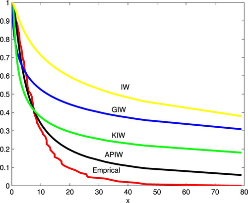
6. Fitting reliability data

In this section, we analyse real data to illustrate that the APIW can be a good lifetime model comparing with many known distributions such as exponentiated (generalized) inverse Weibull (GIW), Kumaraswamy inverse Weibull (KIW) and inverse Weibull (IW) distributions. The real data set in Table 8 represents the remission times (in months) of a random sample of 128 bladder cancer patients reported in Lee and Wang [18].

The next table gives a descriptive summary for these data.

Table 9. Some properties of data set.

Median	Mean	Variance	Skewness	Kurtosis
6.65	9.4437	110.2526	3.2738	18.4421

The parameter of the sample is estimated numerically. We use equations (31(31) $\begin{array}{rl}\frac{\mathrm{\partial }L}{\mathrm{\partial }\alpha }& =\frac{n}{\alpha \log \left(\alpha \right)}-\frac{n}{\alpha -1}+\frac{1}{\alpha }\sum _{i=1}^n{\mathrm{e}}^{-\lambda x_i^{-\text{β}}},\end{array}$(31) )–(33(33) $\begin{array}{rl}\frac{\mathrm{\partial }L}{\mathrm{\partial }\text{β}}& =\frac{n}{\text{β}}-\sum _{i=1}^n\log \left(x_i\right)+\lambda \sum _{i=1}^n{x}_i^{-\text{β}}\log \left(x_i\right)\\ & +\lambda \log \left(\alpha \right)\sum _{i=1}^n{x}_i^{-\text{β}}\log \left(x_i\right){\mathrm{e}}^{-\lambda x_i^{-\text{β}}}.\end{array}$(33) ) to obtain MLEs estimate, Table 10 lists the maximum likelihood estimates of the unknown parameters and the Kolmogorov–Smirnov (K–S) statistics with its corresponding p-value of the APIW and some distributions. Also, from Table 10 the small K–S distance, and the large p-value for the test indicate that these data fit the APIW quite well.

Table 10. Estimates of the parameters and goodness-of-fit tests for data set.

Distributions				Estimates			Statistics
	α	λ	β	θ	a	b	K–S	P-Value
APIW	559.737	0.600494	0.948513	–	–	–	0.1085	0.0921
GIW	-	0.75	0.34	1.797	–	–	0.369	$7.2\times {10}^{-16}$
KIW	-	2.239	3.796	–	0.0077	0.093	0.3402	$1.49\times {10}^{-13}$
IW	-	16.142	0.464	–	–	–	0.503	$4.02\times {10}^{-29}$

Table 11 presents the log-likelihood values (L), Akaike information criterion (AIC), consistent Akaike information criterion (CAIC), Bayesian information criterion (BIC) and Hannan–Quinn information criterion (HQIC) statistics for the fitted APIW and some distributions, where $\begin{array}{rl}\mathrm{A}\mathrm{I}\mathrm{C}& =2k-2L,\mathrm{C}\mathrm{A}\mathrm{I}\mathrm{C}=\mathrm{A}\mathrm{I}\mathrm{C}+\frac{2k(k+1)}{n-k+1},\\ \mathrm{B}\mathrm{I}\mathrm{C}& =k\log \left(n\right)-2L,\mathrm{H}\mathrm{Q}\mathrm{I}\mathrm{C}=2k\log (\log (n\left)\right)-2L,\end{array}$ where n is the sample size and k is the number of parameters. The models with minimum AIC or (−2L, CAIC, BIC, HQIC) value is chosen as the best model to fit the data. From this table, we can conclude that the APIW model provides a better fit to the current data than the other models.

Table 11. Some measures for the fitted models.

Distributions	-2L	AIC	CAIC	BIC	HQIC
APIW	859.007	865.007	865.198	873.563	868.483
GIW	990.360	996.360	996.550	1004.92	999.836
KIW	971.574	979.574	979.894	990.982	984.209
IW	1000.24	1004.24	1004.33	1009.94	1006.56

Figure 7 gives the empirical and fitted reliability functions of selected models. It is clear from these two figures that APIW distribution fit well these data.

Figure 7. The empirical and fitted reliability functions of selected models.

7. Conclusion

In this paper, we introduced our proposed new distribution, named alpha power inverse Weibull. Many properties of our proposed model were investigated, including reliability, moments, entropy and order statistics. The estimation of parameters is obtained by maximum likelihood method. A real data set is applied and has indicated that the proposed new distribution provides flexibility better fit of the data.

Disclosure statement

No potential conflict of interest was reported by the author.

ORCID

Abdulkareem M. Basheer http://orcid.org/0000-0002-3444-6719

References

- Nelson WB. Applied life data analysis. New York (NY): Wiley; 1982.
- Calabria R, Pulcini G. On the maximum likelihood and least Squares estimation in inverse Weibull distribution. Stat Appl. 1990;2:53–66.
- Calabria R, Pulcini G. Bayes 2-Sample prediction for the inverse Weibull distribution. Commun Stat Theory Methods. 1994;23(6):1811–1824. doi: 10.1080/03610929408831356
- Maswadah M. Conditional confidence interval estimation for the inverse Weibull distribution based on censored generalized order statistics. J Stat Comput Simul. 2003;73(12):887–898. doi: 10.1080/0094965031000099140
- Khan MS, Pasha GR, Pasha AH. Theoretical analysis of inverse Weibull distribution. WSEAS Trans Math. 2008;7:30–38.
- Sultan KS, Ismail MA, Al-Moisheer AS. Mixture of two inverse Weibull distributions: properties and estimation. Comput Stat Data Anal. 2007;51:5377–5387. doi: 10.1016/j.csda.2006.09.016
- De Gusmao FRS, Ortega EMM, Cordeiro GM. The generalized inverse Weibull distribution. Stat Papers. 2011;52(3):591-–619. doi: 10.1007/s00362-009-0271-3
- Khan MS, King R. Modified inverse Weibull distribution.J Stat Appl Probab. 2012;1(2):115–132. doi: 10.12785/jsap/010204
- Hanook S, Shahbaz MQ, Mohsin M, et al. A note on beta inverse Weibull distribution. Commun Stat Theory Methods. 2013;42(2):320–335. doi: 10.1080/03610926.2011.581788
- Pararai M, Warahena G, Oluyede BO. A new class of generalized inverse Weibull distribution with applications.J Appl Math Bioinformatics. 2014;4(2):17–35.
- Aryal G, Elbatal I. Kumaraswamy modified inverse Weibull distribution. Appl Math Inf Sci. 2015;9(2):651-–660.
- Elbatal I, Condino F, Domma F. Reflected generalized beta inverse Weibull distribution: definition and properties. Sankhya. 2016;78(2):316–340. doi: 10.1007/s13571-015-0114-2
- Okasha HM, El-Baz AH, Tarabia AMK, et al. Extended inverse Weibull distribution with reliability application.J Egypt Math Soc. 2017;25(3):343–349. doi: 10.1016/j.joems.2017.02.006
- Mahdavi A, Kundu D. A new method for generating distributions with an application to exponential distribution. Commun Stat Theory Methods. 2017;46(13):6543–6557. doi: 10.1080/03610926.2015.1130839
- Kayid M, Izadkhah S. Mean inactivity time function, associated orderings and classes of life distributions. IEEE Trans Reliab. 2014;63(2):593–602. doi: 10.1109/TR.2014.2315954
- Ghitany ME, Atieh B, Nadarajah S. Lindley distribution and its application. Math Comput Simul. 2008;78:493–506. doi: 10.1016/j.matcom.2007.06.007
- Shaked M, Shanthikumar JG. Stochastic orders. New York: Springer; 2007.
- Lee ET, Wang JW. Statistical methods for survival data analysis. 3rd ed. New York: Wiley; 2003.