On weighted exponential-Gompertz distribution: properties and application

Abstract

In this paper, we introduce a new distribution generated by an integral transform of the probability density function of the weighted exponential distribution. This distribution is called the weighted exponential-Gompertz (WE-G). Its hazard rate function can be increasing and bathtub-shaped. Several statistical properties of the new model are obtained, such as moment generating function, moments, conditional moments, mean inactivity time, mean residual lifetime and Rényi entropy. The maximum likelihood estimation of unknown parameters is introduced. A real data application demonstrates the performance of the new model.

KEYWORDS:

• Weighted exponential
• moments
• entropy
• maximum likelihood estimator

MATHEMATICAL SUBJECT CLASSIFICATION (2010):

• 60J65
• 60K40
• 62E10

1. Introduction

Numerous extended distributions have been extensively used over the last decades for modelling data in several areas. Recently, there has been an increased interest in defining new families of distributions by adding one or more parameters to the baseline distribution which provide great flexibility in modelling data in practice. For example, Eugene et al. [1] proposed the beta generated method that uses the beta distribution with parameters $a$ and $b$ as the generator. The cumulative distribution function (cdf) of a beta generated random variable $X$ is defined as (1) $F\left(x\right)=\frac{1}{B(a,b)}{\int }_0^{G\left(x\right)}{t}^{a-1}(1-t{)}^{b-1}dt,a>0,b>0,$(1) where G(x) is the cdf of any random variable X.

Zografos and Balakrishnan [2] have presented a new family of distributions generated by a gamma random variable. This family has the following cdf (2) $F\left(x\right)=\frac{1}{\mathrm{\Gamma }\left(\delta \right)}{\int }_0^{-\log \overline{G}\left(x\right)}{t}^{\delta -1}{\text{e}}^{-t}dt,x\in R,\delta >0,$(2) where $\overline{G}\left(x\right)$ is a survival function which is used to generate a new distribution.

Also, Ristic’ and Balakrishnan [3] introduced a new family of distributions with survival function defined as (3) $\overline{F}\left(x\right)=\frac{1}{\mathrm{\Gamma }\left(\delta \right)}{\int }_0^{-\log G\left(x\right)}{t}^{\delta -1}{\text{e}}^{-t}dt,x,\in R,\delta >0.$(3)

On the same line, we provide a new family of distributions generated by the weighted exponential distribution.

A random variable $X$ has a weighted exponential (WE) distribution if its pdf is given by (4) $f\left(x;\alpha ,\beta \right)=\frac{\alpha +1}{\alpha }\beta {\text{e}}^{-\beta x}\left(1-{\text{e}}^{-\alpha \beta x}\right),x,\alpha ,\beta >0$(4) where $\alpha$ is the shape parameter and $\beta$ is the scale parameter.

The corresponding cdf is (5) $F\left(x;\alpha ,\beta \right)=1-\frac{1}{\alpha }{\text{e}}^{-\beta x}\left(\alpha +1-{\text{e}}^{-\alpha \beta x}\right).$(5)

More details on the WE distribution can be founded in Gupta and Kundu [4].

In this paper, we introduce a new family of distributions generated by an integral transform of the pdf of a random variable $T$ which follows WE distribution. The survival function of this family is defined by $\begin{array}{rl}\overline{F}\left(x;\alpha ,\beta ,\zeta \right)& =\frac{\alpha +1}{\alpha }\beta \underset{0}{\overset{-\log \left[G\left(x;\zeta \right)\right]}{\int }}\left(1-{\text{e}}^{-\alpha \beta t}\right){\text{e}}^{-\beta t}dt\end{array}$ (6) $\begin{array}{rl}& =1-\frac{1}{\alpha }{G}^{\beta }\left(x\right)\left[\alpha +1-G^{\alpha \beta }\left(x\right)\right],\end{array}$(6) and the pdf (7) $\begin{array}{rl}f\left(x;\alpha ,\beta ,\zeta \right)& =\frac{\alpha +1}{\alpha }\beta g\left(x;\zeta \right)G^{\beta -1}\left(x;\zeta \right)\\ & \times \left(1-G^{\alpha \beta }\left(x;\zeta \right)\right),\alpha ,\beta \succ 0\end{array}$(7)

where $G\left(x;\zeta \right)$ and $g\left(x;\zeta \right)$ are the baseline cdf and pdf which depends on a $\left(p\times 1\right)$ parameter vector $\zeta$ and $\left(\alpha ,\beta \right)$ are two additional parameters. Henceforth, we refer this family as WE-G family.

Now we give some motivations for the WE-G family of distributions:

Motivation 1:

In fact, the particular case of Equation (7) for $\alpha =\beta =1$ and $G\left(x\right)=1-e^{-\lambda x}$ with parameter $\lambda >0$ is the exponential with parameter $\eta =2\lambda .$

Motivation 2:

Further, if $\alpha =1$in addition to $G\left(x\right)=x$ for $0<x<1,$ the Equation (7) gives the pdf of Kumaraswamy's distribution with parameters $\left(\beta ,b=2\right).$

Motivation 3:

It is observed that when $\alpha =\beta =1,$ the family (7) reduced to transmuted-G family with parameter $\left(\lambda =1\right)$ proposed by Shaw and Buckley [5] with pdf $f\left(x\right)=2g\left(x;\zeta \right)\left(1-G\left(x;\zeta \right)\right).$

Motivation 4:

Substituting $\alpha =1$ in Equation (7), we obtained the pdf of the generalized transmuted-G family with parameters $\left(\lambda =1,a=b=\beta \right)$ proposed by Nofal et al. [6] as $f\left(x\right)=2\beta g\left(x;\zeta \right)G^{\beta -1}\left(x;\zeta \right)\left(1-G^{\beta }\left(x;\zeta \right)\right).$

Motivation 5:

If we take $\alpha =1,$ the family defined by Equation (7) gives the Kumaraswamy-G family with parameters $\left(a=\beta ,b=1\right)$proposed by Cordeiro and de Castro [7].

In the following sections, we study the properties of a special case of this family, when $G(\cdot )$ is the cdf of the Gompertz distribution. In this case, the random variable $X$ is said to have the weighted exponential-Gompertz distribution.

The reminder of this paper is organized as follows. In Section 2, the weighted exponential-Gompertz distribution is studied in detail. In Section 3, we provide expansions for weighted exponential-Gompertz cumulative and density functions. In Section 4, we present various properties of the new model such as moment generating function, moments and conditional moments. Also, some reliability properties including mean inactivity time function, mean and variance of (reversed) residual lifetime of the our model are discussed in Section 5. In Section 6, Rényi entropy is justified for our proposed model. Order statistics are obtained in Section 7. In Section 8, the maximum likelihood estimator of the parameters of our model is obtained. Section 9 gives an application to a real data set.

2. Weighted exponential-Gompertz distribution

The Gompertz (G) distribution has the pdf (8) $g\left(x;\lambda ,\sigma \right)=\lambda \sigma {\text{e}}^{\lambda x-\sigma \left({\text{e}}^{\lambda x}-1\right)},x\succ 0;\lambda ,\sigma \succ 0$(8) and its cdf is (9) $G\left(x;\lambda ,\sigma \right)=1-{\text{e}}^{-\sigma \left({\text{e}}^{\lambda x}-1\right)}.$(9)

The Gompertz distribution plays an important role in modelling reliability, human mortality and actuarial data that have hazard rate with an exponential increase. An extension version of Gompertz is the weighted Gompertz distribution discussed by Bakouch and Abd El-Bar [8].

From Equations (6–9), we introduce the weighted exponential-Gompertz (WE-G) distribution.

Definition:

A random variable $X$ is said to follow a $\text{WE-G}$ distribution, if its pdf has the form (10) $\begin{array}{rl}& f(x;\alpha ,\beta ,\lambda ,\sigma )\\ & =\frac{(\alpha +1)\beta \sigma \lambda }{\alpha }[{\left(1-{\text{e}}^{-\sigma ({\text{e}}^{\lambda x}-1)}\right)}^{\beta -1}\\ & -{\left(1-{\text{e}}^{-\sigma ({\text{e}}^{\lambda x}-1)}\right)}^{\beta (\alpha +1)}]{\text{e}}^{\lambda x-\sigma ({\text{e}}^{\lambda x}-1)},\end{array}$(10)

and the cdf (11) $\begin{array}{rl}& F(x;\alpha ,\beta ,\lambda ,\sigma )\\ & =\frac{\alpha +1}{\alpha }[1-{\text{e}}^{-\sigma ({\text{e}}^{\lambda x}-1)}{]}^{\beta }\\ & -\frac{1}{\alpha }[1-{\text{e}}^{-\sigma ({\text{e}}^{\lambda x}-1)}{]}^{\beta (\alpha +1)}.\end{array}$(11)

The survival and the hazard rate functions corresponding to (10) are, respectively, defined by (12) $\begin{array}{rl}& S\left(x;\alpha ,\beta ,\lambda ,\sigma \right)\\ & =1-\left(\frac{\alpha +1}{\alpha }{\left[1-{\text{e}}^{-\sigma ({\text{e}}^{\lambda x}-1)}\right]}^{\beta }\right.\\ & \left.-\frac{1}{\alpha }{\left[1-{\text{e}}^{-\sigma ({\text{e}}^{\lambda x}-1)}\right]}^{\beta (\alpha +1)}\right),\end{array}$(12) and

(13) $\begin{array}{r}h\left(x;\alpha ,\beta ,\lambda ,\sigma \right)=\frac{\frac{(\alpha +1)\beta \sigma \lambda }{\alpha }\left[{\left(1-{\text{e}}^{-\sigma ({\text{e}}^{\lambda x}-1)}\right)}^{\beta -1}-{\left(1-{\text{e}}^{-\sigma ({\text{e}}^{\lambda x}-1)}\right)}^{\beta (\alpha +1)}\right]{\text{e}}^{\lambda x-\sigma ({\text{e}}^{\lambda x}-1)}}{1-\left[\frac{\alpha +1}{\alpha }{\left(1-{\text{e}}^{-\sigma ({\text{e}}^{\lambda x}-1)}\right)}^{\beta }-\frac{1}{\alpha }{\left(1-{\text{e}}^{-\sigma ({\text{e}}^{\lambda x}-1)}\right)}^{\beta (\alpha +1)}\right]}.\end{array}$(13)

Figure 1 illustrates the shapes of the pdf of the WE-G distribution for some various values of the shape parameters $\sigma$ and $\alpha$ in the case of $\lambda =2$ and $\beta =1$ for graphs (a), (b), (c) and in the case of $\lambda =1$ and $\beta =2$ for graph (d). It can be summarized some of the shape properties of our model as:

• The pdf is monotonically decreasing when $\sigma <1$ and $\alpha <1$ [graph (a)].

• The pdf is reversed-J when $\sigma \ge 1$ and $\alpha <1$ [graph (b)].

• The pdf is left-skewed when $\sigma <1$ and $\alpha \ge 1$ [graph (c)].

• The pdf is right-skewed when $\sigma >1$ and $\alpha \ge 1$ [graph (d)].

Figure 1. Plots of the density function of WE-G distribution for some values of $\sigma$ and $\alpha .$

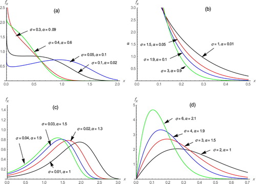
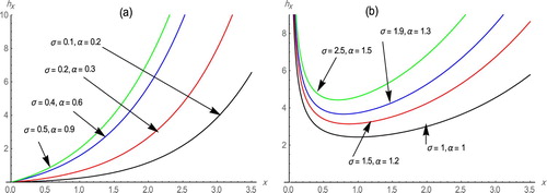
Figure 2 gives some of the possible shapes of the hazard rate function of the WE-G distribution for some various values of the shape parameters $\sigma$ and $\alpha$ in the case of $\lambda =1$ and $\beta =2$ for graph (a) and in the case of $\lambda =0.5$ and $\beta =0.01$ for graph (b). It can be summarized some of the shape properties of the hazard rate function of WE-G as:

• The hazard rate function is an increasing function for $\sigma <1$ and $\alpha <1$ [graph (a)].

• hazard rate function is bathtub shaped for $\sigma \ge 1$ and $\alpha \ge 1$ [graph (b)].

Figure 2. Plots of the hazard rate function of WE-G distribution for some values of $\sigma$ and $\alpha .$

3. Expansions for the cdf and pdf

In this section, we discuss some useful expansions for the cdf and pdf of the $\text{WE - G}$ distribution.

3.1. Expansion for the cdf

In this subsection, we introduce the expansion forms for the cdf for $\text{WE - G}.$

We can express the WE-G cdf as an infinite linear combination of exponentiated Gompertz distribution $\begin{array}{rl}& F(x;\alpha ,\beta ,\lambda ,\sigma )\\ & =\sum _{i=0}^1{(-1)}^i\frac{{\left(\alpha +1\right)}^{(1-i)}}{\alpha }[1-{\text{e}}^{-\sigma ({\text{e}}^{\lambda x}-1)}{]}^{\beta (i\alpha +1)}\end{array}$ (14) $\begin{array}{rl}& =\sum _{i=0}^1{\tau }_{i}G\left(x;\sigma ,\lambda ,\beta (i\alpha +1)\right),\end{array}$(14) where ${\tau }_i=(-1{)}^i\frac{{\left(\alpha +1\right)}^{(1-i)}}{\alpha }$ and $G\left(x;\lambda ,\sigma ,\beta (i\alpha +1)\right)$ denotes the exponentiated Gompertz distribution with parameters $\lambda ,\sigma$ and $\beta (i\alpha +1).$

We also obtain another expansion of the cdf of WE-G as:

From Equation (11) and expanding the term $[1-\exp \left(-\sigma ({\text{e}}^{\lambda x}-1)\right){]}^{\beta (i\alpha +1)},$ the cdf of WE-G can be rewritten as $\begin{array}{rl}F(x;\alpha ,\beta ,\lambda ,\sigma )& =\sum _{i=0}^1\sum _{j=0}^{\mathrm{\infty }}{(-1)}^{i+j}\left(\begin{array}{c}\beta (i\alpha +1)\\ j\end{array}\right)\\ & \times \frac{{\left(\alpha +1\right)}^{(1-i)}}{\alpha }{\text{e}}^{-\sigma j({\text{e}}^{\lambda x}-1)}.\end{array}$

Using power series expansion for $\exp \left(-\sigma j({\text{e}}^{\lambda x}-1)\right)$ and binomial expansion for $({\text{e}}^{\lambda x}-1{)}^k,$ the cdf admits the following expansion (15) $F(x;\alpha ,\beta ,\lambda ,\sigma )=\sum _{i=0}^1\sum _{j,k,m=0}^{\mathrm{\infty }}\sum _{l=0}^k{\omega }_{i,j,k,l}{x}^m,$(15) where $\begin{array}{rl}{\omega }_{i,j,k,l}& =(-1{)}^{i+j+k+l}\left(\begin{array}{c}\beta (i\alpha +1)\\ j\end{array}\right)\left(\begin{array}{c}k\\ l\end{array}\right)\\ & \times \frac{{\left(\sigma j\right)}^k{\left(k-l\right)}^m{\left(\alpha +1\right)}^{(1-i)}}{\alpha k!m!}.\end{array}$

3.2. Expansion for the pdf

Here, we provide simple expansions for the WE-G pdf.

Firstly, expanding the term $[1-\exp (-\sigma ({\text{e}}^{\lambda x}-1)){]}^{\beta (i\alpha +1)-1}$ in Equation (10) yields $\begin{array}{rl}& f(x;\alpha ,\beta ,\lambda ,\sigma )\\ & =\frac{(\alpha +1)\beta \sigma \lambda }{\alpha }{\text{e}}^{\lambda x}\sum _{i=0}^1\sum _{j,k=0}^{\mathrm{\infty }}{(-1)}^{i+j+k}\\ & \times \left(\begin{array}{c}\beta (i\alpha +1)-1\\ j\end{array}\right)\frac{{\left(\sigma \right)}^{k+1}{\left(j+1\right)}^k}{k!}{\left({\text{e}}^{\lambda x}-1\right)}^k.\end{array}$

Using again binomial expansion for $({\text{e}}^{\lambda x}-1{)}^k,$ we can express the pdf of WE-G (16) $f(x;\alpha ,\beta ,\lambda ,\sigma )=\sum _{i=0}^1\sum _{j,k=0}^{\mathrm{\infty }}\sum _{l=0}^k{\upsilon }_{i,j,k,l}\text{exp[}\lambda (k-l+1)x\text{]},$(16) whose weighted coefficients are (17) $\begin{array}{rl}& {\upsilon }_{i,j,k,l}=\frac{(\alpha +1)\beta \sigma \lambda }{\alpha }(-1{)}^{i+j+k+l}\left(\begin{array}{c}\beta (i\alpha +1)-1\\ j\end{array}\right)\\ & \times \left(\begin{array}{c}k\\ l\end{array}\right)\frac{{\left(\sigma \right)}^{k+1}{\left(j+1\right)}^k}{k!}.\end{array}$(17)

We also obtain the expression for the pdf of WE-G as a linear combination of Gompertz density function as: $\begin{array}{rl}& f\left(x;\lambda ,\sigma ,\alpha ,\beta \right)\\ & =\frac{(\alpha +1)\beta \sigma \lambda }{\alpha }\sum _{i=0}^1\sum _{j=0}^{\mathrm{\infty }}{(-1)}^{i+j}\\ & \times \left(\begin{array}{c}\beta (i\alpha +1)-1\\ j\end{array}\right){\text{e}}^{\lambda x-\sigma (j+1)({\text{e}}^{\lambda x}-1)}\end{array}$ (18) $\begin{array}{rl}& =\sum _{j=0}^{\mathrm{\infty }}{\vartheta }_{j}g\left(x;\lambda ,\sigma \left(j+1\right)\right),\end{array}$(18) where ${\vartheta }_j=\frac{(\alpha +1)\beta }{\alpha \left(j+1\right)}(-1{)}^{i+j}\left(\begin{array}{c}\beta (i\alpha +1)-1\\ j\end{array}\right)$ and $g\left(x;\lambda ,\sigma \left(j+1\right)\right)$ denotes the density function of Gompertz distribution with parameters $\lambda$ and $\sigma (j+1).$ Therefore, the density function of WE-G can be expressed as an infinite linear combination of Gompertz densities.

4. Statistical properties of WE-G

In this section, we derive the main statistical properties of $\text{WE-G}$ model for instance, the moment generating function, moments, central moments and conditional moments.

4.1. Moment generating function

Theorem 4.1:

If $X$has the $\text{WE-G}$ distribution, then the moment generating function (mgf) of $X$ is given as follows

(19) $\begin{array}{rl}{M}_X\left(t\right)& =\sum _{i=0}^1\sum _{j,k=0}^{\mathrm{\infty }}\sum _{l=0}^k\frac{{\upsilon }_{i,j,k,l}}{-t-\lambda (k-l+1)};\\ & t+\lambda +k\lambda <l\lambda \end{array}$(19)

where ${\upsilon }_{i,j,k,l}$ defined by Equation (17).

Proof:

The mgf of a continuous random variable $X$ is defined as $M_X\left(t\right)={\int }_0^{\mathrm{\infty }}{\text{e}}^{tx}f\left(x\right)dx.$

Then, the mgf for $\text{WE - G}$ with density function given in Equation (16), we have $\begin{array}{rl}{M}_X\left(t\right)& =\sum _{i=0}^1\sum _{j,k=0}^{\mathrm{\infty }}\sum _{l=0}^k{\upsilon }_{i,j,k,l}\\ & \times {\int }_0^{\mathrm{\infty }}\exp \left[-\left(-t-\lambda (k-l+1)\right)x\right]dx.\end{array}$

Solving the above integral, we have $\begin{array}{rl}{M}_X\left(t\right)& =\sum _{i=0}^1\sum _{j,k=0}^{\mathrm{\infty }}\sum _{l=0}^k\frac{{\upsilon }_{i,j,k,l}}{-t-\lambda (k-l+1)};\\ & \lambda +k\lambda <l\lambda \end{array}$which completes the proof.

4.2. Moments, central moments and conditional moments

Theorem 4.2:

The WE-G random variable has the rth moment function about the origin is (20) ${\mu }_r^{\mathrm{\prime }}=\sum _{i=0}^1\sum _{j,k=0}^{\mathrm{\infty }}\sum _{l=0}^k{\upsilon }_{i,j,k,l}\frac{\mathrm{\Gamma }(r+1)}{{\left(\lambda (l-k-1)\right)}^{r+1}}.$(20)

Proof:

The rth moment about origin is defined by ${\mu }_r^{\mathrm{\prime }}=E\left(X^r\right)={\int }_0^{\mathrm{\infty }}{x}^{r}f\left(x\right)dx.$By using the expansion form of pdf that given in Equation (16) yields $\begin{array}{rl}{\mu }_r^{\mathrm{\prime }}& =\sum _{i=0}^1\sum _{j,k=0}^{\mathrm{\infty }}\sum _{l=0}^k{\upsilon }_{i,j,k,l}{\int }_0^{\mathrm{\infty }}\frac{{\left(\lambda (l-k-1)x\right)}^{r+1-1}}{{\left(\lambda (l-k-1)\right)}^{r+1}}\\ & \times {\text{e}}^{-\lambda (l-k-1)x}d\lambda (l-k-1)x.\end{array}$Since, $\mathrm{\Gamma }\left(r\right)={\int }_0^{\mathrm{\infty }}{y}^{r-1}{\text{e}}^{\text{- y}}dy,$ then the above integral yields the rth moment given by Equation (20).

In particular, the first four moments of $X$ are (21) $\begin{array}{rl}{\mu }_1^{\mathrm{\prime }}& =\sum _{i=0}^1\sum _{j,k=0}^{\mathrm{\infty }}\sum _{l=0}^k{\upsilon }_{i,j,k,l}\frac{1}{\left(\lambda (l-k-1)\right){}^2},\end{array}$(21) $\begin{array}{rl}{\mu }_2^{\mathrm{\prime }}& =\sum _{i=0}^1\sum _{j,k=0}^{\mathrm{\infty }}\sum _{l=0}^k{\upsilon }_{i,j,k,l}\frac{1}{\left(\lambda (l-k-1)\right){}^3},\end{array}$ $\begin{array}{rl}{\mu }_3^{\mathrm{\prime }}& =\sum _{i=0}^1\sum _{j,k=0}^{\mathrm{\infty }}\sum _{l=0}^k{\upsilon }_{i,j,k,l}\frac{1}{{\left(\lambda (l-k-1)\right)}^4},\end{array}$

and ${\mu }_4^{\mathrm{\prime }}=\sum _{i=0}^1\sum _{j,k=0}^{\mathrm{\infty }}\sum _{l=0}^k{\upsilon }_{i,j,k,l}\frac{1}{{\left(\lambda (l-k-1)\right)}^5}.$

Hence, the skewness $\left({\gamma }_1\right)$ and kurtosis $\left({\gamma }_2\right)$ can be obtained using the following relations, ${\gamma }_1=\frac{{\mu }_3^2}{\sqrt{{\left(\mathrm{var}\left(x\right)\right)}^3}}\text{and},{\gamma }_2=\frac{{\mu }_4}{{\left(\mathrm{var}\left(x\right)\right)}^2}$where $\begin{array}{rl}{\mu }_3& ={\mu }_3^{\mathrm{\prime }}-3{\mu }_1^{\mathrm{\prime }}{\mu }_2^{\mathrm{\prime }}+2({\mu }_1^{\mathrm{\prime }}{)}^3\text{and}\\ {\mu }_4& ={\mu }_4^{\mathrm{\prime }}-4{\mu }_1^{\mathrm{\prime }}{\mu }_3^{\mathrm{\prime }}+6({\mu }_1^{\mathrm{\prime }}{)}^2{\mu }_2^{\mathrm{\prime }}-3({\mu }_1^{\mathrm{\prime }}{)}^4.\end{array}$

Proposition 4.1:

Let $X$ be a random variable following the WE-G distribution, then the central moments is (22) $\begin{array}{rl}{\mu }_n& =\sum _{r=0}^n\sum _{i=0}^1\sum _{j,k=0}^{\mathrm{\infty }}\sum _{l=0}^k{\left(-\mu \right)}^{n-r}\left(\begin{array}{c}n\\ r\end{array}\right)\\ & \times {\upsilon }_{i,j,k,l}\frac{\mathrm{\Gamma }(r+1)}{{\left(\lambda (l-k-1)\right)}^{r+1}}.\end{array}$(22)

Proof:

By the definition of central moments, we have (23) ${\mu }_n=E\left[{(x-\mu )}^n\right]=\sum _{r=0}^n\left(\begin{array}{c}n\\ r\end{array}\right){\mu }_r^{\mathrm{\prime }}(-\mu {)}^{n-r}.$(23) Substituting by the Equation (20) into Equation (23) after some simple calculations, we obtain $\begin{array}{rl}{\mu }_n& =\sum _{r=0}^n\sum _{i=0}^1\sum _{j,k=0}^{\mathrm{\infty }}\sum _{l=0}^k{\left(-\mu \right)}^{n-r}\left(\begin{array}{c}n\\ r\end{array}\right)\\ & \times {\upsilon }_{i,j,k,l}\frac{\mathrm{\Gamma }(r+1)}{{\left(\lambda (l-k-1)\right)}^{r+1}}.\end{array}$

Remark 4.1:

The variance of $\text{WE-G}$ model is obtained from Equation (22) for $n=2.$

Note: In the next sections, we will make use of the following lemma.

Lemma 4.1:

Let $\begin{array}{rl}& \varphi \left(z;r,\alpha ,\beta ,\lambda ,\sigma \right)={\int }_0^z{x}^{r}f\left(x;\alpha ,\beta ,\lambda ,\sigma \right)dx\end{array}$ $\begin{array}{rl}& =\sum _{i=0}^1\sum _{j,k=0}^{\mathrm{\infty }}\sum _{l=0}^k{\upsilon }_{i,j,k,l}{\int }_0^{\lambda (l-k-1)z}\frac{{\left(\lambda (l-k-1)x\right)}^{r+1-1}}{{\left(\lambda (l-k-1)\right)}^{r+1}}\\ & \times {\text{e}}^{-\lambda (l-k-1)x}d\lambda (l-k-1)x,\end{array}$

$r=1,2,\dots .$ Then, we have $\begin{array}{rl}& \varphi \left(z;r,\alpha ,\beta ,\lambda ,\sigma \right)\\ & =\sum _{i=0}^1\sum _{j,k=0}^{\mathrm{\infty }}\sum _{l=0}^k{\upsilon }_{i,j,k,l}\gamma (r+1,\lambda z(l-k-1\left)\right),\end{array}$where $\gamma \left(r+1,\lambda z(l-k-1)\right)$ is the lower incomplete gamma function.

Proposition 4.2:

The conditional moments of the WE-G distribution is $\begin{array}{rl}& E\left(X^r|{}_{}X>t\right)\\ & =\frac{\left[E\left(X^r\right)-\varphi \left(t;r,\alpha ,\beta ,\lambda ,\sigma \right)\right]}{1-\left(\frac{\alpha +1}{\alpha }{\left[1-{\text{e}}^{-\sigma ({\text{e}}^{\lambda x}-1)}\right]}^{\beta }-\frac{1}{\alpha }{\left[1-{\text{e}}^{-\sigma ({\text{e}}^{\lambda x}-1)}\right]}^{\beta (\alpha +1)}\right)},\end{array}$

where $E\left(X^r\right)$ is defined by Equation (20) and $\varphi \left(t;r,\alpha ,\beta ,\lambda ,\sigma \right)$ is obtained by Lemma 1.

Proof:

The proof follows from the following definition $E\left(X^r|{}_{}X>t\right)=\frac{1}{S\left(t\right)}\left[E\left(X^r\right)-\underset{0}{\overset{t}{\int }}{x}^{r}f\left(x\right)dx\right].$

5. Reliability measures of WE-G

Here, we derive the expression for the mean and strong mean inactivity time functions, mean and variance of residual lifetime and reversed residual lifetime of the WE-G model.

5.1. Mean inactivity time function

The mean inactivity time (MIT) and strong mean inactivity time (SMIT) functions are an important characteristic in many applications to describe the time, which had elapsed since the failure. Many properties and applications of MIT and SMIT functions can be found in Kayid and Ahmad [9], Izadkhah and Kayid [10] and Kayid and Izadkhah [11]. Let $X$be a lifetime random variable with cdf $F(\cdot ).$ Then the MIT and SMIT respectively, are defined by (24) ${\zeta }_{MIT}\left(t\right)=\frac{1}{F\left(t\right)}\underset{0}{\overset{t}{\int }}F\left(x\right)dx,t>0$(24) and (25) ${\vartheta }_{SMIT}\left(t\right)=\frac{1}{F\left(t\right)}\underset{0}{\overset{t}{\int }}2x_{}F\left(x\right)dx,t>0.$(25)

Proposition 5.1:

The MIT function of $X$ with WE-G distribution is (26) ${\zeta }_{MIT}\left(t\right)=\frac{\sum _{i=0}^1\sum _{j,k,m=0}^{\mathrm{\infty }}\sum _{l=0}^k{\omega }_{i,j,k,l}\frac{t^{m+1}}{m+1}}{\sum _{i=0}^1\sum _{j,k,m=0}^{\mathrm{\infty }}\sum _{l=0}^k{\omega }_{i,j,k,l}{t}^m};t>0.$(26)

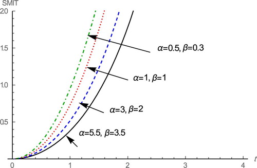
Proposition 5.2:

The SMIT function of $X$ with WE-G distribution is (27) ${\vartheta }_{SMIT}\left(t\right)=\frac{2\sum _{i=0}^1\sum _{j,k,m=0}^{\mathrm{\infty }}\sum _{l=0}^k{\omega }_{i,j,k,l}\frac{t^{m+2}}{m+2}}{\sum _{i=0}^1\sum _{j,k,m=0}^{\mathrm{\infty }}\sum _{l=0}^k{\omega }_{i,j,k,l}{t}^m};t>0.$(27)

From Tables 1 and 2 it is observed that the MIT and SMIT are increasing for decreasing values of $\alpha$ and $\beta ,$ respectively.

Table 1. MIT and SMIT of WE-G distribution.

$\alpha \downarrow$	$t=6,\beta =2,\sigma =1,\lambda =0.5$	MIT	SMIT
5.5		4.54018	33.4294
3.5		4.60215	33.6355
1		4.79335	34.1828
0.5		4.88036	34.3955
0.1		4.98437	34.6253

Table 2. MIT and SMIT of WE-G distribution.

$\beta \downarrow$	$\alpha =\sigma =2.5,\lambda =0.5$	MIT	SMIT
3.5		4.25184	32.5992
2		4.65297	33.7931
1		5.1439	34.894
0.5		5.54717	35.5397
0.1		5.95116	35.9669

From Figures 3 and 4, it is note that MIT and SMIT functions of the WE-G distribution are increasing for decreasing values of $\alpha$ and $\beta$ in the case of $\lambda =0.5,\sigma =1$ and $t=1.$

Figure 3. Plot of MIT function for different values of the parameters $\alpha$ and $\beta .$

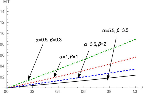
Figure 4. Plot of SMIT function for different values of the parameters $\alpha$ and $\beta .$

5.2. Residual lifetime function

The residual life is the period from time $t$until the time of failure and defined by the conditional random variable $R_{\left(t\right)}:=X-t|X>t,t\ge 0.$

Proposition 5.3:

The mean and variance of $R_{\left(t\right)}$for the WE-G distribution are $\mathrm{K}\left(t\right)=\frac{1}{S\left(t\right)}\left[E\left(X\right)-\varphi \left(t;1,\alpha ,\beta ,\lambda ,\sigma \right)\right]-t,t\ge 0,$and $\begin{array}{rl}\mathrm{\Omega }\left(t\right)& =\frac{1}{S\left(t\right)}\left[E\left(x^2\right)-\varphi \left(t;2,\alpha ,\beta ,\lambda ,\sigma \right)\right]-t^2\\ & -2t_{}\mathrm{K}\left(t\right)-[\mathrm{K}\left(t\right){]}^2,\end{array}$respectively, where $E\left(X\right)$ and $E\left(X^2\right)$ can be obtained using (20),$S\left(t\right)$ defined by (12) and $\varphi \left(t;2,\alpha ,\beta ,\lambda ,\sigma \right)$ is defined by Lemma 1 for $r=2.$

Proof:

The proof follows directly from the definitions: $\mathrm{K}\left(t\right)=E\left(R_{\left(t\right)}\right)=\frac{1}{S\left(t\right)}\underset{t}{\overset{\mathrm{\infty }}{\int }}xf\left(x\right)dx-t,$and $\mathrm{\Omega }\left(t\right)=Var\left(R_{\left(t\right)}\right)=\frac{2}{S\left(t\right)}\underset{t}{\overset{\mathrm{\infty }}{\int }}xS{\left(x\right)}_{}dx-2t_{}\mathrm{K}\left(t\right)-[\mathrm{K}\left(t\right){]}^2.$

5.3. Reversed residual life function

The reversed residual life is the time elapsed from the failure of a component given that its life $X\le t$ and defined as the conditional random variable $\underset{\left(t\right)}{\overset{-}{R}}:=t-X|X\le t.$

Proposition 5.4:

The mean and variance of $\underset{\left(t\right)}{\overset{-}{R}}$for the WE-G distribution are given by $L\left(t\right)=t-\frac{\varphi \left(t;1,\alpha ,\beta ,\lambda ,\sigma \right)}{F\left(t\right)},$and $W\left(t\right)=2t_{}L\left(t\right)-[L\left(t\right){]}^2-t^2+\frac{\varphi \left(t;2,\alpha ,\beta ,\lambda ,\sigma \right)}{F\left(t\right)},$respectively, where $F\left(t\right)$ defined by Equation (11).

Proof:

The proof follows using the following definitions $L\left(t\right)=E\left({\stackrel{-}{R}}_{\left(t\right)}\right)=t-\frac{1}{F\left(t\right)}\underset{0}{\overset{t}{\int }}xf\left(x\right)dx,$

and $\begin{array}{rl}W\left(t\right)& =Var\left({\stackrel{-}{R}}_{\left(t\right)}\right)=2t_{}L\left(t\right)-[L\left(t\right){]}^2\\ & -\frac{2}{F\left(t\right)}\underset{0}{\overset{t}{\int }}xF\left(x\right)dx.\end{array}$

6. Rényi entropy

The entropy of a random variable X is a measure of variation of the uncertainty. The Rényi entropy (Rényi [12]) defined as (28) $I_R\left(\gamma \right)=\frac{1}{1-\gamma }\log \left(\underset{R}{\int }{f}^{\gamma }\left(x\right)dx\right),\gamma >0\text{and}\gamma \ne 1.$(28)

In our case $\begin{array}{rl}{f}^{\gamma }\left(x\right)& ={\left(\frac{(\alpha +1)\beta \sigma \lambda }{\alpha }\right)}^{\gamma }[{\left(1-{\text{e}}^{-\sigma ({\text{e}}^{\lambda x}-1)}\right)}^{\beta -1}\\ & -{\left(1-{\text{e}}^{-\sigma ({\text{e}}^{\lambda x}-1)}\right)}^{\beta (\alpha +1)}{]}^{\gamma }{\text{e}}^{\gamma \lambda x-\gamma \sigma ({\text{e}}^{\lambda x}-1)}.\end{array}$

We expand the following term as $\begin{array}{rl}& [{\left(1-{\text{e}}^{-\sigma ({\text{e}}^{\lambda x}-1)}\right)}^{\beta -1}-{\left(1-{\text{e}}^{-\sigma ({\text{e}}^{\lambda x}-1)}\right)}^{\beta (\alpha +1)}{]}^{\gamma }\\ & =\sum _{i=0}^{\gamma }{(-1)}^i[1-{\text{e}}^{-\sigma ({\text{e}}^{\lambda x}-1)}{]}^{\beta (i\alpha +\gamma )-\gamma }.\end{array}$

Now, applying the power series in the last term of the above equation, we obtain the form of $f^{\gamma }\left(x\right)$ as $f^{\gamma }\left(x\right)=\sum _{i=0}^{\gamma }\sum _{j,k=0}^{\mathrm{\infty }}\sum _{l=0}^k{u}_{i,j,k,l}{\text{e}}^{\lambda \left(\gamma +(k-l)\right)x},$where $u_{i,j,k,l}={\left(\frac{(\alpha +1)\beta \sigma \lambda }{\alpha }\right)}^{\gamma }(-1{)}^{i+j+k+l}\left(\begin{array}{c}k\\ l\end{array}\right)\left(\begin{array}{c}\beta (i\alpha +\gamma )-\gamma \\ j\end{array}\right)\frac{{\left[\sigma (\gamma +j)\right]}^k}{k!}.$

One can evaluate the integral of $f^{\gamma }\left(x\right)$ as $\underset{0}{\overset{\mathrm{\infty }}{\int }}{f}^{\gamma }\left(x\right)dx=\sum _{i=0}^{\gamma }\sum _{j,k=0}^{\mathrm{\infty }}\sum _{l=0}^k{u}_{i,j,k,l}\frac{1}{(l-k-\gamma )\lambda }.$

Then, the Rényi entropy is given by $\begin{array}{rl}& I_R\left(\gamma \right)\\ & =\frac{1}{1-\gamma }\log \left[\sum _{i=0}^{\gamma }\sum _{j,k=0}^{\mathrm{\infty }}\sum _{l=0}^k{u}_{i,j,k,l}\frac{1}{(l-k-\gamma )\lambda }\right]{{,}_{}}_{}^{}\gamma >0.\end{array}$

7. Order statistics

Let $X_1,X_2,\dots ,X_n$ be a random sample from the $\text{WE - G}$ distribution, and let $X_{i:n}$ denote the $ith$ order statistic. The pdf of $ith$ order statistic for ($i=1,2,\dots ,n$), is (29) $f_{i:n}\left(x\right)=\frac{1}{\text{B(}i,n-i+1\text{)}}f\left(x\right)F(x{)}^{i-1}[1-F\left(x\right){]}^{n-i},$(29) where $f(\cdot )$ and $F(\cdot )$ are the pdf and cdf of the WE-G, respectively. Using the definition of binomial expansion for the term: $[1-F\left(x\right){]}^{n-i}$, then $f_{i:n}\left(x\right)$ can be expressed as (30) $f_{i:n}\left(x\right)=\frac{f\left(x\right)}{\text{B(}i,n-i+1\text{)}}\sum _{j=0}^{n-1}{(-1)}^j\left(\begin{array}{c}n-i\\ j\end{array}\right)F(x{)}^{i+j-1}.$(30)

We can write from Equation (11) (31) $\begin{array}{rl}F(x{)}^{i+j-1}& =\sum _{m=0}^{i+j-1}{(-1)}^m\left(\begin{array}{c}i+j-1\\ m\end{array}\right)\\ & \times \frac{1}{{\alpha }^m}{\left(\frac{\alpha +1}{\alpha }\right)}^{i+j-m-1}\\ & \times (1-{\text{e}}^{-\sigma ({\text{e}}^{\lambda x}-1)}{)}^{\beta (i+j-m-1)(\alpha +1)}.\end{array}$(31)

Inserting Equations (10) and (31) in Equation (30), then the pdf of $X_{i:n}$ reduces to

(32) $\begin{array}{rl}{f}_{i:n}\left(x\right)& =\sum _{j=0}^{n-1}\sum _{m=0}^{i+j-1}{\xi }_{j,m}\beta \sigma \lambda {\text{e}}^{\lambda x-\sigma ({\text{e}}^{\lambda x}-1)}\\ & \times {\left[1-{\text{e}}^{-\sigma ({\text{e}}^{\lambda x}-1)}\right]}^{\beta \left[(i+j-m-1)(\alpha +1)+(i\alpha +1)\right]-1},\end{array}$(32) where $\begin{array}{rl}{\xi }_{j,m}& =\sum _{i=0}^1\frac{{(-1)}^{i+j+m}}{\text{B(}i,n-i+1\text{)}}\left(\begin{array}{c}i+j-1\\ m\end{array}\right)\left(\begin{array}{c}n-i\\ j\end{array}\right)\\ & \times \frac{1}{{\alpha }^m}{\left(\frac{\alpha +1}{\alpha }\right)}^{i+j-m}.\end{array}$

Finally, the pdf of $X_{i:n}$ can be expressed as (33) $f_{i:n}\left(x\right)=\sum _{j=0}^{n-1}\sum _{m=0}^{i+j-1}{\varpi }_{j,m}{h}_{\varphi }\left(x\right),$(33) where ${\varpi }_{j,m}=\frac{{\xi }_{j,m}}{\left[(i+j-m-1)(\alpha +1)+(i\alpha +1)\right]},$ $\varphi =\beta \left[(i+j-m-1\left)\right(\alpha +1)+(i\alpha +1)\right]$ and $h_a\left(x\right)=af\left(x\right)F^{a-1}\left(x\right)$ is the exp-G pdf with power parameter $a>0.$ Hence, the pdf of $X_{i:n}$ of a WE-G is a mixture of exp-Gompertz density. So, the moments and mgf of WE-G order statistics follow directly from linear combinations of those quantities for exp-Gompertz distributions, where El-Gohary et al. [13] studied the generalized Gompertz distribution.

8. Estimation and inference

Let $x_1,x_2,\dots ,x_n$ be the random sample from the WE-G with parameters $\alpha ,\beta ,\lambda$ and $\sigma$. Then The log-likelihood function is $\begin{array}{rl}& \begin{array}{c}\ell =n\log \left[\frac{\left(1+\alpha \right)\beta \lambda \sigma }{\alpha }\right]-\sigma \sum _{i=1}^n\left(1-{\text{e}}^{\lambda x_i}\right)+\left(\beta -1\right)\\ \times \sum _{i=1}^n\log \left[1-\text{exp}\left[\sigma (1-{\text{e}}^{\lambda x_i})\right]\right]\end{array}\end{array}$ (34) $\begin{array}{rl}& +\sum _{i=1}^n\log \left[1-{\left(1-\text{exp}\left[\sigma (1-{\text{e}}^{\lambda x_i})\right]\right)}^{\alpha \beta }\right]+\lambda \sum _{i=1}^n{x}_i.\end{array}$(34)

Setting the first derivatives of Equation (34) with respect to $\alpha ,\beta ,\sigma$ and $\lambda$, respectively, to zero, we have

(35) $\begin{array}{rl}\frac{\mathrm{\partial }\ell \left(\mathrm{\Theta }\right)}{\mathrm{\partial }\alpha }& =\frac{n\alpha \left(\frac{\beta \lambda \sigma }{\alpha }-\frac{\left(1+\alpha \right)\beta \lambda \sigma }{{\alpha }^2}\right)}{\left(1+\alpha \right)\beta \lambda \sigma }-\sum _{i=1}^n\frac{{\left(1-\text{exp}\left[\sigma (1-{\text{e}}^{\lambda x_i})\right]\right)}^{\alpha \beta }\beta \log \left[1-\text{exp}\left[\sigma (1-{\text{e}}^{\lambda x_i})\right]\right]}{1-{\left(1-\text{exp}\left[\sigma (1-{\text{e}}^{\lambda x_i})\right]\right)}^{\alpha \beta }}=0,\end{array}$(35) (36) $\begin{array}{rl}\frac{\mathrm{\partial }\ell \left(\mathrm{\Theta }\right)}{\mathrm{\partial }\beta }& =\frac{n}{\beta }+\sum _{i=1}^n\log \left[1-\text{exp}\left[\sigma (1-{\text{e}}^{\lambda x_i})\right]\right]-\sum _{i=1}^n\frac{{\left(1-\text{exp}\left[\sigma (1-{\text{e}}^{\lambda x_i})\right]\right)}^{\alpha \beta }\alpha \log \left[1-\text{exp}\left[\sigma (1-{\text{e}}^{\lambda x_i})\right]\right]}{1-{\left(1-\text{exp}\left[\sigma (1-{\text{e}}^{\lambda x_i})\right]\right)}^{\alpha \beta }}=0,\end{array}$(36) $\begin{array}{rl}\frac{\mathrm{\partial }\ell \left(\mathrm{\Theta }\right)}{\mathrm{\partial }\sigma }& =\frac{n}{\sigma }-\left(\beta -1\right)\sum _{i=1}^n\frac{\text{exp}\left[\sigma (1-{\text{e}}^{\lambda x_i})\right]\left(1-\text{exp}\left[\sigma (1-{\text{e}}^{\lambda x_i})\right]\right)}{1-\text{exp}\left[\sigma (1-{\text{e}}^{\lambda x_i})\right]}-\sum _{i=1}^n\left(\text{exp[}\lambda x_i\text{]}-1\right)\end{array}$ (37) $\begin{array}{rl}& +\sum _{i=1}^n\frac{\text{exp}\left[\sigma (1-{\text{e}}^{\lambda x_i})\right]{\left(1-\text{exp}\left[\sigma (1-{\text{e}}^{\lambda x_i})\right]\right)}^{-1+\alpha \beta }\left(1-\text{exp}\left[\sigma (1-{\text{e}}^{\lambda x_i})\right]\right)\alpha \beta }{1-{\left(1-\text{exp}\left[\sigma (1-{\text{e}}^{\lambda x_i})\right]\right)}^{\alpha \beta }}=0,\end{array}$(37) $\begin{array}{rl}\frac{\mathrm{\partial }\ell \left(\mathrm{\Theta }\right)}{\mathrm{\partial }\lambda }& =\frac{n}{\lambda }+\sum _{i=1}^n{x}_i-\sigma \sum _{i=1}^n{x}_i\text{exp[}\lambda x_i\text{]}+\left(\beta -1\right)\sum _{i=1}^n\frac{\sigma x_i\text{exp[}\lambda x_i\text{ + }\sigma (1-{\text{e}}^{\lambda x_i})\text{]}}{1-\text{exp}\left[\sigma (1-{\text{e}}^{\lambda x_i})\right]}\end{array}$ (38) $\begin{array}{rl}& -\sum _{i=1}^n\frac{\text{exp[}\lambda x_i\text{ + }\sigma (1-{\text{e}}^{\lambda x_i})\text{]}{\left(1-\text{exp}\left[\sigma (1-{\text{e}}^{\lambda x_i})\right]\right)}^{\alpha \beta -1}\alpha \beta \sigma x_i}{1-{\left(1-\text{exp}\left[\sigma (1-{\text{e}}^{\lambda x_i})\right]\right)}^{\alpha \beta }}=0.\end{array}$(38)

The maximum likelihood estimates $\stackrel{⌢}{\alpha },\stackrel{⌢}{\beta },\stackrel{⌢}{\sigma }$ and $\stackrel{⌢}{\lambda }$ can be obtained by solving the non-linear Equations (35–38) numerically for $\alpha ,\beta ,\sigma$ and $\lambda$ by using the statistical software Mathematica package.

For interval estimation of $(\alpha ,\beta ,\sigma ,\lambda )$, we require the information matrix. (39) $I_n=-{\left(\begin{array}{c}{I_{\alpha \alpha }}_{{}_{{}_{}}}{I_{\alpha \beta }}_{{}_{{}_{}}}{I_{\alpha \sigma }}_{{}_{{}_{}}}{I}_{\alpha \lambda }\\ {I_{\beta \alpha }}_{{}_{{}_{}}}{I_{\beta \beta }}_{{}_{{}_{}}}{I_{\beta \sigma }}_{{}_{{}_{}}}{I}_{\beta \lambda }\\ {I_{\sigma \alpha }}_{{}_{{}_{}}}{I_{\sigma \beta }}_{{}_{{}_{}}}{I_{\sigma \sigma }}_{{}_{{}_{}}}{I}_{\sigma \lambda }\\ {I_{\lambda \alpha }}_{{}_{{}_{}}}{I_{\lambda \beta }}_{{}_{{}_{}}}{I_{\lambda \sigma }}_{{}_{{}_{}}}{I}_{\lambda \lambda }\end{array}\right)}_{\alpha =\stackrel{}{\stackrel{⌢}{\alpha }{,}_{}\beta =\stackrel{}{\stackrel{⌢}{\beta }{,}_{}\sigma =\stackrel{}{\stackrel{⌢}{\sigma }{,}_{}\lambda =\stackrel{⌢}{\lambda }}}}},$(39) where the elements of the matrix $I_n(\alpha ,\beta ,\sigma ,\lambda )$ are given in the Appendix.

The variance-covariance matrix would be $I_n^{-1}(\alpha ,\beta ,\sigma ,\lambda ),$ where $I_n^{-1}(\alpha ,\beta ,\sigma ,\lambda )$ is the inverse of the observed information matrix.

9. Data application

In this section, we provide a practical example to illustrate the perform of the new model. To illustrate the good performance of our model, we use package Mathematica software. For comparison purpose, we consider the following distributions: Gompertz $\left(\text{G}(\sigma ,\lambda )\right)$ distribution: $g\left(x\right)=\lambda \sigma \text{exp}\left[\lambda x-\sigma \left({\text{e}}^{\lambda x}-1\right)\right],x,\sigma ,\lambda >0.$

• Shifted Gompertz $\left(\text{S}\text{G}\text{(}a\text{,}b\text{)}\right)$ distribution (Bemmaor [14]): $\begin{array}{rl}g\left(x\right)& =a\text{exp[}-ax-b{\text{e}}^{-ax}\text{]}\left[\text{1}+b\left(1-{\text{e}}^{-ax}\right)\right],\\ & xa,b>0.\end{array}$

• Weighted exponential-log logistic $\left(\text{WE -LL}\text{(}\alpha \text{,}\beta \text{,}\eta \text{,}\kappa )\right)$ distribution:

$\begin{array}{r}g\left(x\right)=\frac{\left(1+\alpha \right)\beta \eta \left({\left[1-1/\left(1+{\left(x/\kappa \right)}^{\eta }\right)\right]}^{\beta }-{\left[1-1/\left(1+{\left(x/\kappa \right)}^{\eta }\right)\right]}^{\left(1+\alpha \right)\beta }\right)}{\alpha \left(1+{\left(x/\kappa \right)}^{\eta }\right)x},x,\alpha \text{,}\beta \text{,}\eta \text{,}\kappa >0.\end{array}$

• Weighted exponential-Weibull $\left(\text{WE-W(}\alpha \text{,}\beta \text{,}\theta \text{,}\gamma \text{)}\right)$ distribution:

$\begin{array}{rl}& g\left(x\right)=\frac{\left(\alpha +1\right)\beta \theta \gamma \left[{\left(1-{\text{e}}^{-\gamma x^{\theta }}\right)}^{\beta }-{\left(1-{\text{e}}^{-\gamma x^{\theta }}\right)}^{\left(\alpha +1\right)\beta }\right]x^{\theta -1}}{\alpha \left({\text{e}}^{\gamma x^{\theta }}-1\right)},x,\alpha \text{,}\beta \text{,}\theta \text{,}\gamma >0.\end{array}$

The data set represents the failure time of 50 devices (Aarset [15]) and listed in Table 3. For Aarset data, we obtain the maximum likelihood estimates (MLE's) and the respective standard errors of each distribution. Further, we use the goodness-of – fit statistics in order to provide the Akaike Information Criterion (AIC), Bayesian Information Criterion (BIC) and Hannan-Quinn Information Criterion (HQIC), Kolmogorov-Smirnov (K-S) test, the p-value of K-S, Cramer-von Misses ($W^{\ast }$) and Anderson Darling ($A^{\ast }$). Table 4 provides the MLE's and the respective standard errors for comparison distributions. Tables 5 and 6 provides the values of AIC, BIC, HQIC, K-S, p- value, W* and A* of the comparison distributions. Hence, we conclude that our model provides the better fit. Figure 5 shows the estimated densities and estimated survival functions for the considered distributions of data set. We note that the proposed model is more appropriated to fit the data, again. We also, plot the profiles of the log-likelihood function in Figures 6–9 to show that the likelihood equations have a unique solution in the parameters of WE-G distributions. Some descriptive statistics of the Aarset data can be found in Table 7, that indicates negative skewness and kurtosis.

Figure 5. (a) Estimated density function and (b) Estimated survival function of Aarset data.

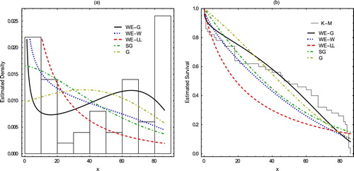
Figure 6. The profiles of the log-likelihood function of $\alpha$.

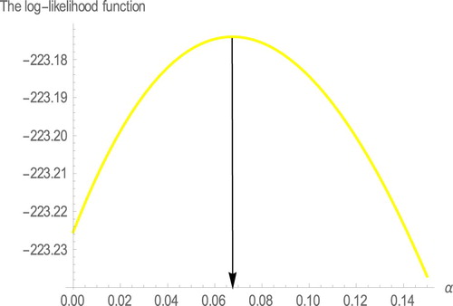
Figure 7. The profiles of the log-likelihood function of $\beta$.

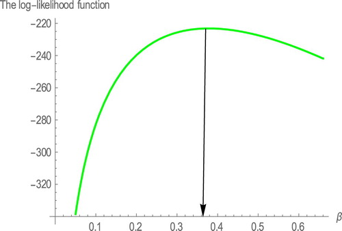
Figure 8. The profiles of the log-likelihood function of $\sigma .$

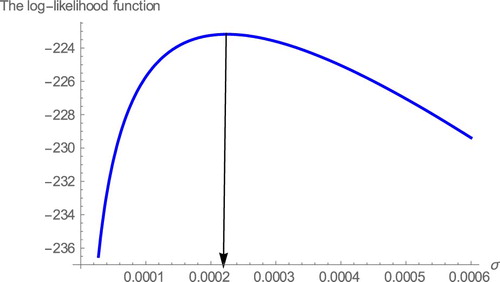
Figure 9. The profiles of the log-likelihood function of $\lambda$.

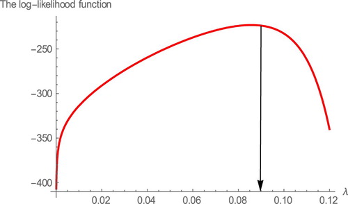
Table 3. Aarset data set.

0.1	0.2	1	1	1	1	1	2	3	6	7	11	12
18	18	18	18	18	21	32	36	40	45	46	47	50
55	60	63	63	67	67	67	67	72	75	79	82	82
83	84	84	84	85	85	85	85	85	86	86

Table 4. MLEs of the parameters (standard errors in parentheses).

Models		Estimates
$\text{WE -G(}\alpha \text{,}\beta \text{,}\sigma \text{,}\lambda \text{)}$	$\stackrel{⌢}{\alpha }=0.06797$	$\stackrel{⌢}{\beta }=0.37863$	$\stackrel{⌢}{\sigma }=0.00022$	$\stackrel{⌢}{\lambda }=0.08566$
	(3.45949)	(0.58538)	(0.00063)	(0.00063)
$\text{WE-W(}\alpha \text{,}\beta \text{,}\theta \text{,}\gamma \text{)}$	$\stackrel{⌢}{\alpha }=11.49690$	$\stackrel{⌢}{\beta }=0.26102$	$\stackrel{⌢}{\theta }=2.68462$	$\stackrel{⌢}{\gamma }=4.3977\times {10}^{-6}$
	(7.33062)	(0.08528)	(0.76146)	(0.00002)
$\text{WE-LL(}\alpha \text{,}\beta \text{,}\eta \text{,}\kappa \text{)}$	$\stackrel{⌢}{\alpha }=11.68650$	$\stackrel{⌢}{\beta }=0.79576$	$\stackrel{⌢}{\eta }=1.06442$	$\stackrel{⌢}{\kappa }=29.87580$
	(6.66497)	(0.22712)	(0.24325)	(10.9208)
$\text{SG(}a\text{,}b\text{)}$	–	–	$\stackrel{⌢}{a}=0.02601$	$\stackrel{⌢}{b}=0.44871$
			(0.00452)	(0.40200)
$\text{G}(\sigma ,\lambda )$	–	–	$\stackrel{⌢}{\sigma }=0.00972$	$\stackrel{⌢}{\lambda }=0.02030$
			(0.00300)	(0.00601)

Table 5. AIC, BIC and HQIC statistics.

Models	AIC	BIC	HQIC
$\text{WE - G(}\alpha \text{,}\beta \text{,}\sigma \text{,}\lambda \text{)}$	454.348	461.996	457.260
$\text{WE - W(}\alpha \text{,}\beta \text{,}\theta \text{,}\gamma \text{)}$	470.109	477.757	473.022
$\text{WE - LL(}\alpha \text{,}\beta \text{,}\eta \text{,}\kappa \text{)}$	503.780	511.429	506.693
$\text{SG(}a\text{,}b\text{)}$	484.848	488.672	486.305
$\text{G}(\sigma ,\lambda )$	474.662	478.486	476.118

Table 6. W*, A* statistics, K-S statistic and it’s corresponding p-value.

Distribution	W*	A*	K-S	p-value
$\text{WE -G(}\alpha \text{,}\beta \text{,}\sigma \text{,}\lambda \text{)}$	0.22487	1.60354	0.14241	0.26256
$\text{WE - W(}\alpha \text{,}\beta \text{,}\theta \text{,}\gamma \text{)}$	0.52324	3.17609	0.20176	0.03413
$\text{WE -LL(}\alpha \text{,}\beta \text{,}\eta \text{,}\kappa \text{)}$	1.20922	6.21649	0.28941	0.00046
$\text{SG(}a\text{,}b\text{)}$	1.17045	10.8511	0.28443	0.00061
$\text{G}(\sigma ,\lambda )$	0.46758	4.80357	0.16969	0.11230

Table 7. Descriptive statistics – Aarest data.

Minimum	0.1
Maximum	86
Mean	45.686
Median	48.5
SD	32.835
MD-mean	29.6191
MD-median	29.554
Skewness	–0.13644
Kurtosis	–1.61441

The observed information of the Aarset data and the variance-covariance matrices are respectively $\begin{array}{rl}& I(\alpha ,\beta ,\sigma ,\lambda )\\ & =\left(\begin{array}{c}{20.58}_{{}_{{}_{}}}{119.50}_{{}_{{}_{}}}-{38266.38}_{{}_{{}_{}}}-416.55\\ \text{119}\text{.5}{\text{0}}_{{}_{{}_{}}}\text{696}\text{.7}{\text{9}}_{{}_{{}_{}}}-\text{21859}{\text{3}}_{{}_{{}_{}}}-2337.88\\ -{38266.4}_{{}_{{}_{}}}-{218.59}_{{}_{{}_{}}}1.89\times {{10}^8}_{{}_{{}_{}}}3.32\times {10}^6\\ -416.545-2337.883.32\times {10}^{6}64686.1\end{array}\right),\end{array}$and $\begin{array}{rl}& I^{-1}(\alpha ,\beta ,\sigma ,\lambda )\\ & =\left(\begin{array}{c}{11.968}_{{}_{{}_{}}}-{1.9904}_{{}_{{}_{}}}{0.00032}_{{}_{{}_{}}}-0.01113\\ \text{ - 1}\text{.990}{\text{3}}_{{}_{{}_{}}}{0.3427}_{{}_{{}_{}}}9.469\times {{10}^{-6}}_{{}_{{}_{}}}-0.00092\\ {0.0003}_{{}_{{}_{}}}9.469\times {{10}^{-6}}_{{}_{{}_{}}}3.944\times {{10}^{-7}}_{{}_{{}_{}}}-0.00018\\ -0.0111-0.0009-0.0000180.00083\end{array}\right).\end{array}$

The 90% confidence intervals (CIs) for the parameters $\alpha ,\beta ,\sigma$ and$\lambda$are (0, 5.75831 ], (0, 1.3415], (0, 0.0012579) and [0.0384075, 0.132916 ], respectively.

10. Concluding remarks

In this paper, a new extension version of the Gompertz distribution generated by integral transform of the pdf of the weighted exponential distribution is introduced with its important properties. Estimation using the method of maximum likelihood is straightforward. Moreover, the new model with other distributions is fitted to real data set and it is shown that this model has a better performance among the compared distributions. Some issues for future research may be considering different estimation methods of the unknown parameters. In addition, the new model properties can be compared with process based on two-piece distributions (Maleki and Mahmoudi [16] and Hoseinzadeh et al. [17]).

Disclosure statement

No potential conflict of interest was reported by the authors.

Appendix

The elements of the $4\times 4$ observed information matrix $I_n=I_n\left(\alpha ,\beta ,\sigma ,\lambda \right)$ are: $\begin{array}{rl}{I}_{\alpha \alpha }& =\frac{n\alpha \left(-\frac{2\beta \lambda \sigma }{{\alpha }^2}+\frac{2\left(1+\alpha \right)\beta \lambda \sigma }{{\alpha }^3}\right)}{\left(1+\alpha \right)\beta \lambda \sigma }-\frac{n\alpha \left(\frac{\beta \lambda \sigma }{\alpha }-\frac{\left(1+\alpha \right)\beta \lambda \sigma }{{\alpha }^2}\right)}{{\left(1+\alpha \right)}^2\beta \lambda \sigma }\\ & +\frac{n\left(\frac{\beta \lambda \sigma }{\alpha }-\frac{\left(1+\alpha \right)\beta \lambda \sigma }{{\alpha }^2}\right)}{\left(1+\alpha \right)\beta \lambda \sigma }\end{array}$ $\begin{array}{rl}& -\sum _{i=1}^n\left(\frac{{\left(1-u_i\right)}^{2\alpha \beta }{\beta }^2\text{Log}{\left[1-u_i\right]}^2}{{\left(1-{\left(1-u_i\right)}^{\alpha \beta }\right)}^2}\right)\\ & -\sum _{i=1}^n\frac{{\left(1-u_i\right)}^{\alpha \beta }{\beta }^2\text{Log}{\left[1-u_i\right]}^2}{1-{\left(1-u_i\right)}^{\alpha \beta }},\end{array}$ $\begin{array}{rl}{I}_{\alpha \beta }& =\frac{n\alpha \left(\frac{\lambda \sigma }{\alpha }-\frac{\left(1+\alpha \right)\lambda \sigma }{{\alpha }^2}\right)}{\left(1+\alpha \right)\beta \lambda \sigma }-\frac{n\alpha \left(\frac{\beta \lambda \sigma }{\alpha }-\frac{\left(1+\alpha \right)\beta \lambda \sigma }{{\alpha }^2}\right)}{\left(1+\alpha \right){\beta }^2\lambda \sigma }\\ & -\sum _{i=1}^n\frac{{\left(1-u_i\right)}^{\alpha \beta }\text{Log}\left[1-u_i\right]}{1-{\left(1-u_i\right)}^{\alpha \beta }}\end{array}$ $\begin{array}{rl}& -\alpha \beta \sum _{i=1}^n\frac{{\left(1-u_i\right)}^{2\alpha \beta }\text{Log}{\left[1-u_i\right]}^2}{{\left(1-{\left(1-u_i\right)}^{\alpha \beta }\right)}^2}\\ & -\alpha \beta \sum _{i=1}^n\frac{{\left(1-u_i\right)}^{\alpha \beta }\text{Log}{\left[1-u_i\right]}^2}{1-{\left(1-u_i\right)}^{\alpha \beta }},\end{array}$ $\begin{array}{rl}{I}_{\alpha \sigma }& =\frac{n\alpha \left(\frac{\beta \lambda }{\alpha }-\frac{\left(1+\alpha \right)\beta \lambda }{{\alpha }^2}\right)}{\left(1+\alpha \right)\beta \lambda \sigma }-\frac{n\alpha \left(\frac{\beta \lambda \sigma }{\alpha }-\frac{\left(1+\alpha \right)\beta \lambda \sigma }{{\alpha }^2}\right)}{\left(1+\alpha \right)\beta \lambda {\sigma }^2}\\ & +\beta \sum _{i=1}^n\frac{u_i{\left(1-u_i\right)}^{\alpha \beta -1}\left(1-u_i\right)}{1-{\left(1-u_i\right)}^{\alpha \beta }}\end{array}$ $\begin{array}{rl}& +\alpha {\beta }^2\sum _{i=1}^n\frac{u_i{\left(1-u_i\right)}^{-1+2\alpha \beta }\left(1-{\text{e}}^{\lambda x_i}\right)\text{Log}\left[1-u_i\right]}{{\left(1-{\left(1-u_i\right)}^{\alpha \beta }\right)}^2}\\ & +\alpha {\beta }^2\sum _{i=1}^n\frac{u_i{\left(1-u_i\right)}^{-1+\alpha \beta }{h}_i\text{Log}\left[1-u_i\right]}{1-{\left(1-u_i\right)}^{\alpha \beta }},\end{array}$ $\begin{array}{rl}{I}_{\alpha \lambda }& =\frac{n\alpha \left(\frac{\beta \sigma }{\alpha }-\frac{\left(1+\alpha \right)\beta \sigma }{{\alpha }^2}\right)}{\left(1+\alpha \right)\beta \lambda \sigma }-\frac{n\alpha \left(\frac{\beta \lambda \sigma }{\alpha }-\frac{\left(1+\alpha \right)\beta \lambda \sigma }{{\alpha }^2}\right)}{\left(1+\alpha \right)\beta {\lambda }^2\sigma }\\ & -\beta \sigma \sum _{i=1}^n\frac{x_i{\left(1-u_i\right)}^{\alpha \beta -1}{v}_i}{1-{\left(1-u_i\right)}^{\alpha \beta }}\end{array}$ $\begin{array}{rl}& +\alpha \sigma {\beta }^2\sum _{i=1}^n\frac{x_i{\left(1-u_i\right)}^{2\alpha \beta -1}\text{Log}\left[1-u_i\right]v_i}{{\left(1-{\left(1-u_i\right)}^{\alpha \beta }\right)}^2}\end{array}$ $\begin{array}{rl}& -\alpha \sigma {\beta }^2\sum _{i=1}^n\frac{x_i{\left(1-u_i\right)}^{\alpha \beta -1}\text{Log}\left[1-u_i\right]v_i}{1-{\left(1-u_i\right)}^{\alpha \beta }},\end{array}$ $\begin{array}{rl}{I}_{\beta \beta }& =-\frac{n}{{\beta }^2}-{\alpha }^2\sum _{i=1}^n\frac{{\left(1-u_i\right)}^{2\alpha \beta }\text{Log}{\left[1-u_i\right]}^2}{{\left(1-{\left(1-u_i\right)}^{\alpha \beta }\right)}^2}\\ & -{\alpha }^2\sum _{i=1}^n\frac{{\left(1-u_i\right)}^{\alpha \beta }\text{Log}{\left[1-u_i\right]}^2}{1-{\left(1-u_i\right)}^{\alpha \beta }},\end{array}$ $\begin{array}{rl}{I}_{\beta \sigma }& =-\sum _{i=1}^n\frac{u_i{h}_i}{1-u_i}+\sum _{i=1}^n\frac{u_i{\left(1-u_i\right)}^{-1+\alpha \beta }{h}_i\alpha }{1-{\left(1-u_i\right)}^{\alpha \beta }}\\ & +{\alpha }^2\beta \sum _{i=1}^n\frac{u_i{\left(1-u_i\right)}^{2\alpha \beta -1}{h}_i\text{Log}\left[1-u_i\right]}{{\left(1-{\left(1-u_i\right)}^{\alpha \beta }\right)}^2}\end{array}$ $\begin{array}{rl}& +{\alpha }^2\beta \sum _{i=1}^n\frac{u_i{\left({\left(1-u_i\right)}^{\alpha \beta }\right)}^{\alpha \beta -1}{h}_i\text{Log}\left[{\left(1-u_i\right)}^{\alpha \beta }\right]}{1-{\left({\left(1-u_i\right)}^{\alpha \beta }\right)}^{\alpha \beta }},\end{array}$ $\begin{array}{rl}{I}_{\beta \lambda }& =\sigma \sum _{i=1}^n\frac{v_i{x}_i}{1-u_i}-\alpha \sigma \sum _{i=1}^n\frac{v_i{\left(1-u_i\right)}^{\alpha \beta -1}{x}_i}{1-{\left(1-u_i\right)}^{\alpha \beta }}\\ & -{\alpha }^2\beta \sigma \sum _{i=1}^n\frac{v_i{\left(1-u_i\right)}^{2\alpha \beta -1}\text{Log}\left[1-u_i\right]x_i}{{\left(1-{\left(1-u_i\right)}^{\alpha \beta }\right)}^2}\end{array}$ $\begin{array}{rl}& -{\alpha }^2\beta \sigma \sum _{i=1}^n\frac{v_i{\left(1-u_i\right)}^{2\alpha \beta -1}\text{Log}\left[1-u_i\right]x_i}{{\left(1-{\left(1-u_i\right)}^{\alpha \beta }\right)}^2}\\ & -{\alpha }^2\beta \sigma \sum _{i=1}^n\frac{v_i{\left(1-u_i\right)}^{\alpha \beta -1}\text{Log}\left[1-u_i\right]x_i}{1-{\left(1-u_i\right)}^{\alpha \beta }},\end{array}$ $\begin{array}{rl}{I}_{\sigma \sigma }& =-\frac{n}{{\sigma }^2}-\left(\beta -1\right)\sum _{i=1}^n\left(\frac{\text{exp}\left[2\sigma h_i\right]{h_i}^2}{{\left(1-u_i\right)}^2}+\frac{u_i{h_i}^2}{1-u_i}\right)\\ & +\alpha \beta \sum _{i=1}^n\frac{u_i{\left(1-u_i\right)}^{\alpha \beta -1}{h_i}^2}{1-{\left(1-u_i\right)}^{\alpha \beta }}\end{array}$ $\begin{array}{rl}& -{\alpha }^2{\beta }^2\sum _{i=1}^n\frac{\text{exp}\left[2\sigma h_i\right]{\left(1-u_i\right)}^{2\alpha \beta -2}{h_i}^2}{{\left(1-{\left(1-u_i\right)}^{\alpha \beta }\right)}^2}\\ & -\alpha \beta \left(\alpha \beta -1\right)\sum _{i=1}^n\frac{\text{exp}\left[2\sigma h_i\right]{\left(1-u_i\right)}^{\alpha \beta -2}{h_i}^2}{1-{\left(1-u_i\right)}^{\alpha \beta }},\\ I_{\sigma \lambda }& =-\sum _{i=1}^n{\text{e}}^{\lambda x_i}{x}_i+\left(\beta -1\right)\sum _{i=1}^n\frac{v_i{x}_i}{1-u_i}\\ & -\sum _{\text{i}=1}^{\text{n}}\frac{v_i{\left(1-u_i\right)}^{\alpha \beta -1}\left(1-u_i\right)\alpha \beta \sigma x_i}{1-{\left(1-u_i\right)}^{\alpha \beta }}\end{array}$ $\begin{array}{rl}& +\left(\beta -1\right)\sum _{i=1}^n\frac{\text{exp[2}\sigma h_i+\lambda x_i\text{]}{h}_i\sigma x_i}{{\left(1-u_i\right)}^2}\\ & +\left(\beta -1\right)\sum _{i=1}^n\frac{v_i{h}_i\sigma x_i}{1-u_i}\\ & -\sum _{i=1}^n\frac{v_i{\left(1-u_i\right)}^{\alpha \beta -1}\alpha \beta x_i}{1-{\left(1-u_i\right)}^{\alpha \beta }}\end{array}$ $\begin{array}{rl}& +\sum _{\text{i}=1}^{\text{n}}\frac{\text{exp[2}\sigma h_i+\lambda x_i\text{]}{\left(1-u_i\right)}^{2\alpha \beta -2}{h}_i{\alpha }^2{\beta }^2\sigma x_i}{{\left(1-{\left(1-u_i\right)}^{\alpha \beta }\right)}^2}\end{array}$ $\begin{array}{rl}& +\sum _{i=1}^n\frac{\text{exp[2}\sigma h_i+\lambda x_i\text{]}{\left(1-u_i\right)}^{\alpha \beta -2}{h}_i\alpha \beta \left(-1+\alpha \beta \right)\sigma x_i}{1-{\left(1-u_i\right)}^{\alpha \beta }},\end{array}$

and $\begin{array}{rl}{I}_{\lambda \lambda }& =-\frac{n}{{\lambda }^2}-\sigma \sum _{i=1}^n{x_i}^2{\text{e}}^{\lambda x_i}\\ & -\left(\beta -1\right)\sum _{i=1}^n\frac{\text{exp[2}\sigma h_i+2\lambda x_i\text{]}{\sigma }^2{x_i}^2}{{\left(1-u_i\right)}^2}\end{array}$ $\begin{array}{rl}& +\left(\beta -1\right)\sum _{i=1}^n\frac{v_i\sigma x_i(x_i-{\text{e}}^{\lambda x_i}\sigma x_i)}{1-u_i}\\ & -\sum _{i=1}^n\frac{\text{exp[2}\sigma h_i+2\lambda x_i\text{]}{\left(1-u_i\right)}^{2\alpha \beta -2}{\alpha }^2{\beta }^2{\sigma }^2{x_i}^2}{{\left(1-{\left(1-u_i\right)}^{\alpha \beta }\right)}^2}\end{array}$ $\begin{array}{rl}& -\alpha \beta \left(\alpha \beta -1\right){\sigma }^2\\ & \sum _{\text{i}=1}^{\text{n}}\frac{\text{exp[2}\sigma h_i+2\lambda x_i\text{]}{\left(1-u_i\right)}^{\alpha \beta -2}{x_i}^2}{1-{\left(1-u_i\right)}^{\alpha \beta }}\end{array}$ $\begin{array}{rl}& -\sum _{i=1}^n\frac{v_i{\left(1-u_i\right)}^{\alpha \beta -1}\alpha \beta \sigma x_i\left(x_i-{\text{e}}^{\lambda x_i}\sigma x_i\right)}{1-{\left(1-u_i\right)}^{\alpha \beta }},\end{array}$where $\begin{array}{rl}{u}_i& =u_i\left(\lambda ,\sigma \right)=\exp \left[\sigma \left(1-e^{\lambda x_i}\right)\right]{{,}_{}}_{}{v}_i=v_i\left(\lambda ,\sigma \right)=\exp [\sigma \\ & \left(1-e^{\lambda x_i}\right)+\lambda x_i]\text{and}{h}_i=h_i(\lambda )=(1-e^{\lambda x_i}).\end{array}$

References

- Eugene N, Lee C, Famoye F. Beta-normal distribution and its applications. Communi Stat Theory Methods. 2002;31:497–512. doi: 10.1081/STA-120003130
- Zografos K, Balakrishnan N. On families of beta-and generalized gamma-generated distributions and associated inference. Stat Methodol. 2009;6:344–362. doi: 10.1016/j.stamet.2008.12.003
- Ristic MM, Balakrishnan N. The gamma-exponentiated exponential distribution. J Stat Comput Simul. 2012;82:1191–1206. doi: 10.1080/00949655.2011.574633
- Gupta RD, Kundu D. A new class of weighted exponential distribution. Statistics. 2009;43:621–634. doi: 10.1080/02331880802605346
- Shaw WT, Buckley IR. The alchemy of probability distribution: beyond Gram-Charlier expansions, and a skew-kurtotic-normal distribution from a rank transmutation map. Tech Rep. 2009. Available from http://arxiv.org/abs/0901.0434.
- Nofal ZM, Afify AZ, Yousof HM, et al. The generalized transmuted-G family of distributions. Communi Stat Theory Methods. 2016. doi:10.1080/03610926.2015.1078478.
- Cordeiro GM, De Castro M. A new family of generalized distributions. J Stat Comput Simul. 2011;81:883–893. doi: 10.1080/00949650903530745
- Bakouch HS, Abd El-Bar AMT. A new weighted Gompertz distribution with applications to reliability data. Appl Math. 2017;62:269–296. doi: 10.21136/AM.2017.0277-16
- Kayid M, Ahmad IA. On the mean inactivity time ordering with reliability applications. Prob Eng Inform Sci. 2004;18:395–409. doi: 10.1017/S0269964804183071
- Izadkhan S, Kayid M. Reliability analysis of the harmonic mean inactivity time order. IEEE Trans Reliab. 2013;62:329–337. doi: 10.1109/TR.2013.2255793
- Kayid M, Izadkhah S. Mean inactivity time function, associated orderings and classes of life distribution. IEEE Trans Reliab. 2014;63:593–602. doi: 10.1109/TR.2014.2315954
- Rényi A. On measures of entropy and information. In Proceedings of the 4th Berkeley symposium on Mathematical Statistics and Probability I. 1961. Berkeley: Univ. California Press. MR0132570; p. 547–561.
- El-Gohary A, Alshamrani A, Al-Otaibi AN. The generalized Gompertz distribution. Appl Math Modeling. 2013;37:13–24. doi: 10.1016/j.apm.2011.05.017
- Bemmaor AC. Modeling the diffusion of new durable goods: word-of-mouth effect versus consumer heterogeneity. In: B Pras, editor. Research traditions in marketing. Boston, MA: Kluwer; 1994. p. 201–223.
- Aarset MV. How to identify bathtub hazard rate. IEEE Trans Reliab. 1987;36:106–108. doi: 10.1109/TR.1987.5222310
- Maleki M, Mahmoudi MR. Two-piece location-scale distributions based on scale mixtures of normal family. Communi Stat Theory Methods. 2017;46:12356–12369. doi: 10.1080/03610926.2017.1295160
- Hoseinzadeh A, Maleki M, Khodadadi Z, et al. The skew-reflected- Gompertz distribution for analyzing symmetric and asymmetric data. J Comput Appl Math. 2019;349:132–141. doi: 10.1016/j.cam.2018.09.011
Appendix
The elements of the observed information matrix