Full article: Defining a curve as a Bezier curve

Formulae display: $MathJax Logo$ ?Mathematical formulae have been encoded as MathML and are displayed in this HTML version using MathJax in order to improve their display. Uncheck the box to turn MathJax off. This feature requires Javascript. Click on a formula to zoom.

Abstract

A Bezier curve is significant with its control points. When control points are given, the Bezier curve can be written using De Casteljau's algorithm. An important property of Bezier curve is that every coordinate function is a polynomial. Suppose that a curve $α (t)$ is a curve which coordinate functions are polynomial. Can we find points that make the curve $α (t)$ as Bezier curve? This article presents a method for finding points which present $α (t)$ as a Bezier curve.

KEYWORDS:

AMS SUBJECT CLASSIFICATIONS:

1. Introduction

The curve theory is used in differential geometry, kinematics, robotics and engineering. Bezier curves are important subset of the curves. Bezier curves have been used in computer-aided geometric design (CAGD) and in many areas [Citation1–5]. For every Bezier curve, the control points are uniquely defined [Citation6]. In CAGD, the most popular areas of research are used shape control parameters to construct Bezier curves [Citation7]. It is possible to establish the linear relationship of the control points of a Bezier curve and surface [Citation8, Citation9]. It is well known from the relevant literature, a Bezier curve is established by the control points. When the control points are given, using the Bernstein polynomial and De Castaljeu algorithm we can write the Bezier curve.

The coordinates of a Bezier curve are polynomial functions including the coefficients of Bernstein polynomial and the component of the control points. However, when a Bezier curve is given, we can not say the control points what are? In the relevant literature, there are some articles about finding the control points of third order with minimum error [Citation10].

Our aim is to find the control points exactly, not approximately. Suppose that $α (t)$ is a curve, $α_{1} (t)$ , $α_{2} (t)$ , $α_{3} (t)$ are coordinate functions. $α_{1} (t)$ , $α_{2} (t)$ , $α_{3} (t)$ are polynomial with degree $m_{1,}$ $m_{2}$ and $m_{3}$ , respectively. In this case, we can find $max {m_{1}, m_{2}, m_{3}} + 1$ points which are control points of the curve $α (t)$ as a Bezier curve. The original contribution of our study is to find the control points when a curve is given. We need only the coefficients of polynomial coordinate functions. These coefficients give us the coordinates of control points using the inverse of creator matrix. Creator matrix has an inverse. We show this case in Section 3. The advantages of the proposed method are different from the existing methods. The control points are given for finding the Bezier curve in the existing methods but the control points are found in our method. If we have creator matrix, we can find the control points every time.

Firstly, we give basic knowledge about a Bezier curve. And then, we introduce a method to find the control points of a given curve in Section 3, which is the original part of this article.

2. Preliminaries

Binomial expansion with n-degree for a and b is given by $(a + b)^{n} = \sum_{i = 0}^{n} (\binom{n}{i}) a^{i} b^{n - i} .$ For a=t and b=1−t, we can write this polynomial, which is called Bernstein polynomial, as $B (t) = \sum_{i = 0}^{n} (\binom{n}{i}) t^{i} (1 - t)^{n - i}, 0 \leq t \leq 1$ or $B_{n} (t) = \sum_{i = 0}^{n} B_{i}^{n} (t),$ where $B_{i}^{n} (t) = (\binom{n}{i}) t^{i} (1 - t)^{n - i}$ . This polynomial was introduced by Bernstein [Citation11]. A Bernstein polynomial can be written in matrix form [Citation12].

Bernstein polynomials have the linearly independent property, so Bernstein polynomials set ${B_{i}^{n}}$ forms a basis for all polynomials. Using the de Casteljau algorithm and Bernstein polynomial, a Bezier curve can be written as (1) $B Z (t) = \sum_{i = 0}^{n} (\binom{n}{i}) t^{i} (1 - t)^{n - i} P_{i}, 0 \leq t \leq 1,$ (1) where $P_{i}$ are elements of $R^{k}$ , $k \leq n$ , and called Bezier points [Citation13].

If $P_{i} = (P_{i x}, P_{i y}, P_{i z}) \in R^{3},$ $0 \leq i \leq n,$ then we have $B Z (t) = \sum_{i = 0}^{n} B_{i}^{n} (t) (P_{i x}, P_{i y}, P_{i z})$ and, in terms of coordinate functions, (2) $B Z (t) = (\sum_{i = 0}^{n} B_{i}^{n} (t) P_{i x}, \sum_{i = 0}^{n} B_{i}^{n} (t) P_{i y}, \sum_{i = 0}^{n} B_{i}^{n} (t) P_{i z}) .$ (2) $B Z (t)$ is continuous on $[a, b]$ and differentiable on $(a, b)$ .

Using the matrix form, we can write a Bezier curve with $(n + 1) -$ control points as $B Z (t) = [B_{i}^{n}] . P,$ where $P = [P_{i}]_{_{(n + 1) \times 1}}$ and $P_{i} = (P_{i x}, P_{i y}, P_{i z})$ are the control points of the Bezier curve $B Z (t)$ in $R^{3}$ .

3. Calculating the points for a curve $α (t)$ which makes as Bezier curve

3.1. Creator matrix

In this section, we give a matrix formulation to calculate the unknown control points of a given curve.

In generally, a Bezier curve is not written in the power basis ${t^{i}}$ . However, for calculating the control points of a Bezier curve, $B Z (t)$ must be written in the power basis ${t^{i}}$ . In Equation (1), the multipliers of each component $(\binom{n}{i}) t^{i} (1 - t)^{n - i} P_{i}$ belongs to N, $T_{t},$ $T_{(1 - t)}$ and P, where $\begin{aligned} N & = ((\binom{n}{0}) (\binom{n}{1}) (\binom{n}{2}) \dots (\binom{n}{k}) \dots (\binom{n}{n - 1}) (\binom{n}{n})), \\ T_{t} & = (t^{0} t^{1} t^{2} \dots t^{k} \dots t^{n - 1} t^{n}), \\ T_{(1 - t)} & = ((1 - t)^{n} \dots (1 - t)^{n - k} \dots (1 - t)^{n - (n - 1)} \\ (1 - t)^{n - (n - 0)}), \\ P & = (P_{0} P_{1} P_{2} \dots P_{k} \dots P_{n - 1} P_{n}) . \end{aligned}$

Hence, we can write $B Z (t) = \sum_{i = 0}^{n} N_{i} . (T_{t})_{i} . (T_{(1 - t)})_{n - i} . P_{i} .$ The serial expansion of every $(1 - t)^{(n - i)}$ placed in $T_{(1 - t)}$ is as $(1 - t)^{n - i} = \sum_{j = 0}^{n - i} (\binom{n - i}{j}) (- 1)^{j} t^{j} .$ In this case, $B Z (t)$ can be written in the power basis { $t^{i}$ }. Now we have to calculate the coefficients of $t^{i}$ . The coefficients of $t^{i}$ can be obtained from the following statements, respectively; $\begin{aligned} t^{n} \{(\binom{n}{0}) (\binom{n}{n}) (- 1)^{n} P_{0} + (\binom{n}{1}) (\binom{n - 1}{n - 1}) (- 1)^{n - 1} P_{1} + \dots \\ + (\binom{n}{n}) (\binom{n - n}{n - n}) (- 1)^{n - n} P_{n}\}, \\ t^{n - 1} \{(\binom{n}{0}) (\binom{n}{n - 1}) (- 1)^{n - 1} P_{0} + \dots + (\binom{n}{n - 1}) \\ \times (\binom{n - (n - 1)}{n - (n - 1) - 1}) (- 1)^{n - (n - 1) - 1} P_{n - 1}\}, \\ t^{n - 2} \{(\binom{n}{0}) (\binom{n}{n - 2}) (- 1)^{n - 2} P_{0} + \dots + (\binom{n}{n - 2}) \\ \times (\binom{n - (n - 2)}{n - (n - 2) - 2}) (- 1)^{n - (n - 2) - 2} P_{n - 2}\}, \\ t^{n - 3} \{(\binom{n}{0}) (\binom{n}{n - 3}) (- 1)^{n - 3} P_{0} + \dots + (\binom{n}{n - 3}) \\ \times (\binom{n - (n - 3)}{n - (n - 3) - 3}) (- 1)^{n - (n - 3) - 3} P_{n - 3}\}, \\ ⋮ \\ t^{3} \{(\binom{n}{0}) (\binom{n}{3}) (- 1)^{3} P_{0} + (\binom{n}{1}) (\binom{n - 1}{2}) (- 1)^{2} P_{1} + \dots \\ + (\binom{n}{3}) (\binom{n - 3}{0}) (- 1)^{0} P_{3}\}, \\ t^{2} \{(\binom{n}{0}) (\binom{n}{2}) (- 1)^{2} P_{0} + (\binom{n}{1}) (\binom{n - 1}{1}) (- 1)^{1} P_{1} \\ + (\binom{n}{2}) (\binom{n - 2}{0}) (- 1)^{0} P_{2}\}, \\ t^{1} \{(\binom{n}{0}) (\binom{n}{1}) (- 1)^{1} P_{0} + (\binom{n}{1}) (\binom{n - 1}{0}) (- 1)^{0} P_{1}\}, \\ t^{0} \{(\binom{n}{0}) (\binom{n}{0}) (- 1)^{0} P_{0}\} . \end{aligned}$

Using the coefficients of $t^{n}, \dots, t^{1}, t^{0}$ , the curve (3) $B Z (t) = \sum_{i = 0}^{n} (\binom{n}{i}) t^{i} (1 - t)^{n - i} P_{i}, P_{i} = (P_{i x}, P_{i y}, P_{i z})$ (3) can be written as (4) $B Z (t) = \sum_{i = 0}^{n} t^{i} \{\sum_{j = 0}^{n - i} (\binom{n}{j}) (\binom{n - j}{i - j}) (- 1)^{i - j} P_{j}\} .$ (4) Equation (4) is the main equation for this article. In Equation (4), the Bezier curve $B Z (t)$ is written in matrix form as follows (5) $B Z (t) = T . A . P,$ (5) where, (6) $\begin{aligned} T & = [t^{i}], i = 0, \dots, n, \\ A & = [a_{i j}], a_{i j} = (\binom{n}{j}) (\binom{n - j}{i - j}) (- 1)^{i - j}, \\ P & = [P_{i}], i = 0, \dots, n . \end{aligned}$ (6)

Now we give a new definition.

Definition 3.1

The matrix $A = [a_{i j}] = [(\binom{n}{j}) (\binom{n - j}{i - j}) (- 1)^{i - j}]$ is called the creator matrix for Bezier curves.

3.2. Finding the control points

The creator matrix and the given Bezier curve in the form $B Z (t) = T . A . P$ are very important. Since in this case, the matrix A is invertible and this allows us to find the control points of unknown control points of a Bezier curve. Also, using Equation (5), it is very easy to calculate the derivative and integration of a Bezier curve. Now we give a proposition, theorem and examples using the creator matrix.

Proposition 3.2

The creator matrix A is an invertible matrix.

Proof.

A is a lower-triangle square matrix and $det A = \prod_{i = 0}^{n} a_{i i}$ . For $\forall i$ , $a_{i i} = (\binom{n}{i}) (\binom{n - i}{i - i}) (- 1)^{i - i} = (\binom{n}{i}) \neq 0.$ That is, $d e t A \neq 0$ .

Theorem 3.3

Every curve which coordinate functions are polynomial can be written as a Bezier curve.

Proof.

When a curve is given with the coordinate functions to be polynomial, there are the control points uniquely and exactly which they make the curve as Bezier curve. Suppose that any polynomial curve $C (t)$ is given by $C : I ⟶ R^{n}$ , n=2 or n=3, $I = [0, 1],$ (7) $C (t) = (\sum_{i = 0}^{n} C_{i x} t^{i}, \sum_{i = 0}^{n} C_{i y} t^{i}, \sum_{i = 0}^{n} C_{i z} t^{i}) .$ (7) Then, $C (t)$ can be written in matrix form as (8) $C (t) = [\begin{matrix} t^{0} & t^{1} & t^{2} & \dots & t^{n} \end{matrix}] [\begin{matrix} C_{0 x} & C_{0 y} & C_{0 z} \\ C_{1 x} & C_{1 y} & C_{1 z} \\ C_{2 x} & C_{2 y} & C_{2 z} \\ ⋮ & ⋮ & ⋮ \\ C_{n x} & C_{n y} & C_{n z} \end{matrix}] .$ (8) From Equations (5) and (8), we have $A [\begin{matrix} P_{0 x} & P_{0 y} & P_{0 z} \\ P_{1 x} & P_{1 y} & P_{1 z} \\ P_{2 x} & P_{2 y} & P_{2 z} \\ ⋮ & ⋮ & ⋮ \\ P_{n x} & P_{n y} & P_{n z} \end{matrix}] = [\begin{matrix} C_{0 x} & C_{0 y} & C_{0 z} \\ C_{1 x} & C_{1 y} & C_{1 z} \\ C_{2 x} & C_{2 y} & C_{2 z} \\ ⋮ & ⋮ & ⋮ \\ C_{n x} & C_{n y} & C_{n z} \end{matrix}]$ and (9) $\begin{aligned} A [\begin{matrix} P_{0 x} \\ P_{1 x} \\ P_{2 x} \\ ⋮ \\ P_{n x} \end{matrix}] = [\begin{matrix} C_{0 x} \\ C_{1 x} \\ C_{2 x} \\ ⋮ \\ C_{n x} \end{matrix}], A [\begin{matrix} P_{0 y} \\ P_{1 y} \\ P_{2 y} \\ ⋮ \\ P_{n y} \end{matrix}] = [\begin{matrix} C_{0 y} \\ C_{1 y} \\ C_{2 y} \\ ⋮ \\ C_{n y} \end{matrix}], A [\begin{matrix} P_{0 z} \\ P_{1 z} \\ P_{2 z} \\ ⋮ \\ P_{n z} \end{matrix}] \\ = [\begin{matrix} C_{0 z} \\ C_{1 z} \\ C_{2 z} \\ ⋮ \\ C_{n z} \end{matrix}] . \end{aligned}$ (9) So, we find the solutions of Equation (9) as (10) $\begin{aligned} [\begin{matrix} P_{0 x} \\ P_{1 x} \\ P_{2 x} \\ ⋮ \\ P_{n x} \end{matrix}] = A^{- 1} [\begin{matrix} C_{0 x} \\ C_{1 x} \\ C_{2 x} \\ ⋮ \\ C_{n x} \end{matrix}], \\ [\begin{matrix} P_{0 y} \\ P_{1 y} \\ P_{2 y} \\ ⋮ \\ P_{n y} \end{matrix}] = A^{- 1} [\begin{matrix} C_{0 y} \\ C_{1 y} \\ C_{2 y} \\ ⋮ \\ C_{n y} \end{matrix}], \\ [\begin{matrix} P_{0 z} \\ P_{1 z} \\ P_{2 z} \\ ⋮ \\ P_{n z} \end{matrix}] = A^{- 1} [\begin{matrix} C_{0 z} \\ C_{1 z} \\ C_{2 z} \\ ⋮ \\ C_{n z} \end{matrix}] . \end{aligned}$ (10)

This solution is unique. This method gives us the control points exactly, not approximately.

Example

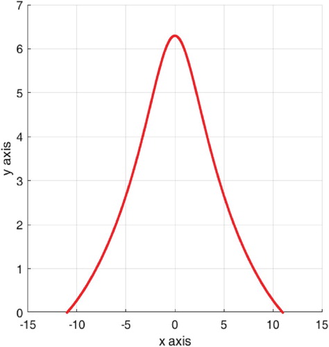
Suppose that a Bezier curve is given as $\begin{aligned} C (t) & : I ⟶ R^{2}, \\ C (t) & = (C_{1} (t), C_{2} (t)), \end{aligned}$ where, $\begin{aligned} C_{1} (t) & = - 180 t^{9} + 810 t^{8} - 1800 t^{7} + 2520 t^{6} - 2268 t^{5} \\ + 1260 t^{4} - 360 t^{3} + 40 t - 11, \\ C_{2} (t) & = - 52 t^{10} + 260 t^{9} - 270 t^{8} - 480 t^{7} \\ + 1260 t^{6} - 1008 t^{5} + 420 t^{4} - 240 t^{3} \\ + 90 t^{2} + 10 t \end{aligned}$ (Figure ).

Figure 1. The curve $C (t)$ .

Now we calculate the control points of the curve $C (t)$ . For this we write the programme in Matlab.

Coefficients matrix of this curve is $C = [\begin{matrix} - 11 & 0 \\ 40 & 10 \\ 0 & 90 \\ - 360 & - 240 \\ 1260 & 420 \\ - 2268 & - 1008 \\ 2520 & 1260 \\ - 1800 & - 480 \\ 810 & - 270 \\ - 180 & 260 \\ 0 & - 52 \end{matrix}]$ From $P = A^{- 1} C$ , we have $P = [\begin{matrix} - 11 & 0 \\ - 7 & 1 \\ - 3 & 3 \\ - 2 & 5 \\ - 1 & 7 \\ 0 & 8 \\ 1 & 7 \\ 2 & 5 \\ 3 & 3 \\ 7 & 1 \\ 11 & 0 \end{matrix}] .$ The control points are $\begin{aligned} p_{0} = (- 11, 0), p_{1} = (- 7, 1), p_{2} = (- 3, 3), \\ p_{3} = (- 2, 5), p_{4} = (- 1, 7), p_{5} = (0, 8), \\ p_{6} = (1, 7), p_{7} = (2, 5), p_{8} = (3, 3), p_{9} = (7, 1), \\ p_{10} = (11, 0) . 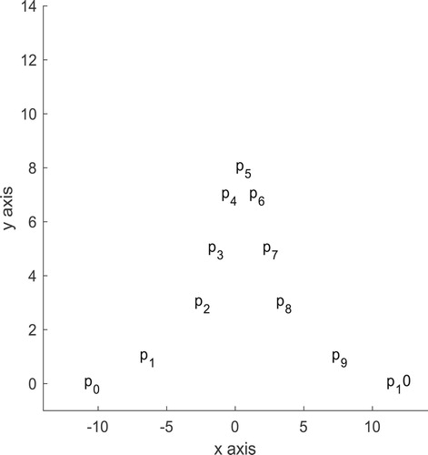\end{aligned}$ The control points of $C (t)$ is drawn as in Figure . At the end we can plot Bezier curve, the control points and the control polygon of curve $C (t)$ (Figure ).

Figure 2. The control points of $C (t)$ .

Example

Let curve $β (t)$ be given as follows. $\begin{aligned} β (t) = 3665 t^{10} + 16300 t^{9} - 24750 t^{8} + 9000 t^{7} \\ + 15750 t^{6} - 21420 t^{5} + 11550 t^{4} - 3000 t^{3} \\ + 225 t^{2} + 20, \\ 5 t (- 1380 t^{9} + 7260 t^{8} - 16965 t^{7} + 22920 t^{6} - 19110 t^{5} \\ + 9576 t^{4} - 2520 t^{3} + 120 t^{2} + 135 t - 40), \\ 5 t^{2} (- 211 t^{8} + 2356 t^{7} - 8550 t^{6} + 15720 t^{5} - 16800 t^{4} \\ + 10836 t^{3} - 3990 t^{2} + 600 t) + 45) . \end{aligned}$

The figure of this curve is as in Figure .

Figure 3. Bezier curve, the control points and the control polygon of $C (t)$ .

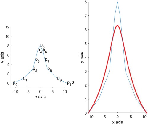
Figure 4. The curve $β (t)$ .

The coefficients matrix of $β (t)$ is $C = [\begin{matrix} 20 & 0 & 0 \\ 0 & - 200 & 0 \\ 225 & - 675 & 225 \\ - 3000 & - 600 & 3000 \\ 11550 & 12600 & - 19950 \\ - 21420 & - 47880 & 54180 \\ 15750 & 95550 & - 84000 \\ 9000 & - 114600 & 78600 \\ - 24750 & - 84825 & - 42750 \\ 16300 & - 36300 & 11780 \\ - 3665 & 6900 & - 1055 \end{matrix}] .$ The creator matrix is $\begin{aligned} A = [\begin{matrix} 1 & 0 & 0 & 0 & 0 \\ - 10 & 10 & 0 & 0 & 0 \\ 45 & - 90 & 45 & 0 & 0 \\ - 120 & 360 & - 360 & 120 & 0 \\ 210 & - 840 & 1260 & - 840 & 210 \\ - 252 & 1260 & - 2520 & 2520 & - 1260 \\ 210 & - 1260 & 3150 & - 4200 & 3150 \\ - 120 & 840 & - 2520 & 4200 & - 4200 \\ 45 & - 360 & 1260 & - 2520 & 3150 \\ - 10 & 90 & - 360 & 840 & - 1260 \\ 1 & - 10 & 45 & - 120 & 210 \end{matrix} \\ \begin{matrix} 0 & 0 & 0 & 0 & 0 0 \\ 0 & 0 & 0 & 0 & 0 0 \\ 0 & 0 & 0 & 0 & 0 0 \\ 0 & 0 & 0 & 0 & 0 0 \\ 0 & 0 & 0 & 0 & 0 0 \\ 252 & 0 & 0 & 0 & 0 0 \\ - 1260 & 210 & 0 & 0 & 0 0 \\ 2520 & - 840 & 120 & 0 & 0 0 \\ - 2520 & 1260 & - 360 & 45 & 0 0 \\ 1260 & - 840 & 360 & - 90 & 10 0 \\ - 252 & 210 & - 120 & 45 & - 10 1 \end{matrix}] . \end{aligned}$ The inverse of the creator matrix is $\begin{aligned} A^{- 1} = [\begin{matrix} 1 & 0 & 0 & 0 & 0 & 0 \\ 1 & 0.1 & 0 & 0 & 0 & 0 \\ 1 & 0.2 & 0.0222 & 0 & 0 & 0 \\ 1 & 0.3 & 0.0667 & 0.0083 & 0 & 0 \\ 1 & 0.4 & 0.1333 & 0.0333 & 0.0048 & 0 \\ 1 & 0.5 & 0.2222 & 0.0833 & 0.0238 & 0.004 \\ 1 & 0.6 & 0.3333 & 0.1667 & 0.0714 & 0.0238 \\ 1 & 0.7 & 0.4667 & 0.2917 & 0.1667 & 0.0833 \\ 1 & 0.8 & 0.6222 & 0.4667 & 0.3333 & 0.2222 \\ 1 & 0.9 & 0.8 & 0.7 & 0.6 & 0.5 \\ 1 & 1 & 1 & 1 & 1 & 1 \end{matrix} \\ \begin{matrix} 0 & 0 & 0 & 0 0 \\ 0 & 0 & 0 & 0 0 \\ 0 & 0 & 0 & 0 0 \\ 0 & 0 & 0 & 0 0 \\ 0 & 0 & 0 & 0 0 \\ 0 & 0 & 0 & 0 0 \\ 0.0048 & 0 & 0 & 0 0 \\ 0.0333 & 0.0083 & 0 & 0 0 \\ 0.1333 & 0.0667 & 0.0222 & 0 0 \\ 0.4 & 0.3 & 0.2 & 0.1 0 \\ 1 & 1 & 1 & 1 1 \end{matrix}] . 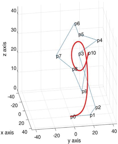\end{aligned}$ So we have the control points from $P = A^{- 1} C .$ The control points are $\begin{aligned} p_{0} & = (20, 0, 0), p_{1} = (20, 20, 0), p_{2} = (25, 25, 5), \\ p_{3} & = (10, 10, 30), \\ p_{4} & = (5, 30, 35), p_{5} = (10, 10, 40), p_{6} = (- 15, 10, 40), \\ p_{7} & = (- 10, - 10, 25), \\ p_{8} & = (0, 5, 20), p_{9} = (0, 15, 8), p_{10} = (10, 20, 30) . \end{aligned}$

The control points of $β (t)$ are shown as in Figure .The control polygon of the Bezier curve is drawn as in Figure . Finally, we can draw the Bezier curve as in Figure .

Figure 5. The control points of $β (t)$ .

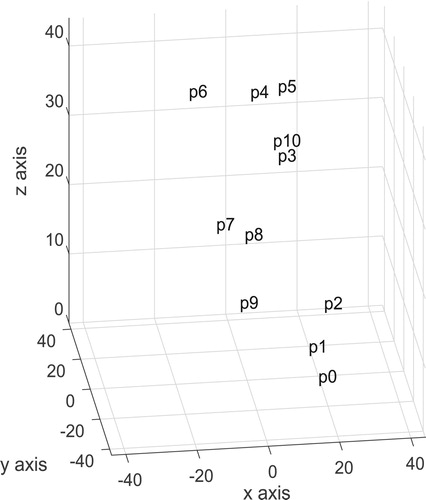
Figure 6. The control polygon of the Bezier curve.

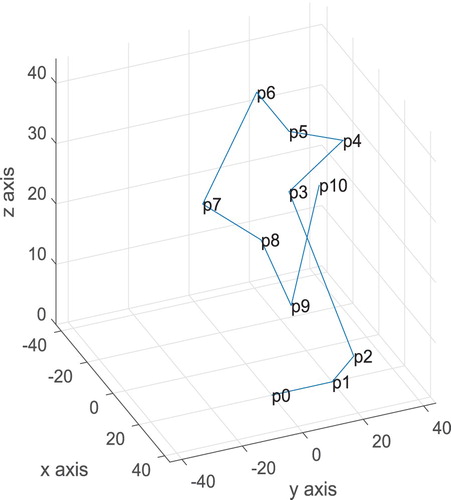
Figure 7. The Bezier curve according to the control points.

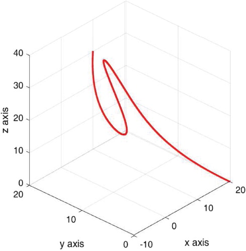
Example

Let the curve $γ (t)$ be given in $R^{4}$ as $\begin{aligned} γ (t) & = (6 + 3 t - 2 t^{2} + 8 t^{3} + 11^{4}, - t + 7 t^{3} + 15 t^{4}, \\ - 5 + 20 t + 11 t^{2} + 20 t^{3} - 2 t^{4}, 5 t + 17 t^{2} \\ + 20 t^{3} + 18 t^{4}) . \end{aligned}$ The coefficients matrix of $γ (t)$ is $C = [\begin{matrix} 6 & 0 & - 5 & 0 \\ 3 & - 4 & 20 & 5 \\ 2 & 0 & 11 & 17 \\ 8 & 7 & 20 & 20 \\ 11 & 15 & - 2 & 18 \\ 12 & 15 & 18 & 23 \end{matrix}] .$ The creator matrix A and the inverse of the creator matrix B are as follows. $A = [\begin{matrix} 1 & 0 & 0 & 0 & 0 & 0 \\ - 5 & 5 & 0 & 0 & 0 & 0 \\ 10 & - 20 & 100 & 0 & 0 & 0 \\ - 10 & 30 & - 30 & 10 & 0 & 0 \\ 5 & - 20 & 30 & - 20 & 5 & 0 \\ - 1 & 5 & - 10 & 10 & 5 & 1 \end{matrix}]$ and $B = [\begin{matrix} 1 & 0 & 0 & 0 & 0 & 0 \\ 1 & 0.2 & 0 & 0 & 0 & 0 \\ 1 & 0.4 & 0.1 & 0 & 0 & 0 \\ 1 & 0.6 & 0.3 & 0.1 & 0 & 0 \\ 1 & 0.8 & 0.6 & 0.4 & 0.2 & 0 \\ 1 & 1 & 1 & 1 & 1 & 1 \end{matrix}] .$ Thus we have the control points of $γ (t)$ as a Bezier curve is found as $p_{0} = (6, 0, - 5, 0),$ $\begin{aligned} p_{1} & = (6.6, - 0.8, - 1, 1), p_{2} = (7.4, - 1.6, 4.1, 3.7), \\ p_{3} = (9.2, 1.7, 12.3, 10.1), \\ p_{4} & = (15, 2.6, 25.2, 25.8), p_{5} = (42, 33, 62, 83) . \end{aligned}$

3.3. Derivative and integration on the Bezier curves

It is notable that if Bezier curve can be written as in Equation (5), this new argument can raise many advantages. For example, in case a representation as in Equation (5) it can be easily calculated the derivative, integration,…,etc of the Bezier curve. This is a clear advantage of writting a Bezier curve in matrix form. Here, we success this fact for Bezier curves. In addition, in the relevant literature the derivative and integration of various Bezier curves are calculated by classical ways. This case brings many difficulties. However, in this paper we calculate the derivative of the Bezier curves by means of the matrix form. This case can bring many advantages for the researchers. That is, in that case, we can calculate the derivative and integration of the Bezier curves easily. These are the contributions of this paper to the literature and its novelty and originality. This method, which defines the Bezier curve as the polynomial in the power basis ${t^{i}}$ , is very useful in practice and computer science. Suppose that the Bezier curve with $n -$ control points is given as in Equation (5), $B Z (t) = T . A . P .$ In this case, the derivative of $B Z (t)$ is $\frac{d (B Z (t))}{d t} = \frac{d T}{d t} . A . P$

and $\frac{d T}{d t} = [0, 1, 2 t, 3 t^{2}, \dots, k t^{k - 1}, \dots, n t^{n - 1}] .$ We can calculate the successive derivative $\frac{d^{k} (B Z (t))}{d^{k} t},$ $1 \leq k \leq n .$

Furthermore, we can calculate easily the integration of a Bezier curve using the form in Equation (5). So, the integration of $B Z (t)$ is $\int B Z (t) d t = (\int T d t) A . P .$

4. Conclusion

In computer-aided geometric design (CAGD), one of the main problem is to calculate the control points of a Bezier curve with unknown control points. In this article, a matrix is defined and called a creator matrix. The product of creator matrix of the control points gives us the Bezier curve. Conversely, since the creator matrix is invertible, inverse of the creator matrix can be used to find the control points of the Bezier curve.

Disclosure statement

No potential conflict of interest was reported by the authors.

References

Bezier P. The mathematical basis of the UNISURF CAD system. London: Butterworths; 1986.
Google Scholar
Bezier P. Mathematical and practical possibilities of UNISURF. Comput Aided Geom Design. 1974;127–152. doi: 10.1016/B978-0-12-079050-0.50012-6
Google Scholar
Boehm W, Muller A. On de Castejau's algorithm. Comput Aided Geom Design. 1999;16:587–605. doi: 10.1016/S0167-8396(99)00023-0
Google Scholar
Farin G. Curves and surfaces for computer aided geometric design. Boston: Academic Press; 1993.
Google Scholar
Farin G. Curves and surfaces for CAGD. Boston: Academic Press; 2002.
Google Scholar
Berry TG, Patterson RR. The uniqueness of Bezier control points. Comput Aided Geom Design. 1997;14:877–879. doi: 10.1016/S0167-8396(97)00016-2
Web of Science ®Google Scholar
Qin X, Hu G, Zhang N, et al. A novel extension to the polynomial basis functions describing Bezier curves and surfaces of degree n with multiple shape parameters. Appl Math Comput. 2013;223:1–16.
Web of Science ®Google Scholar
Deng J, Kao T. Linear relationship of the control points of Bezier curve for degree reduction: a tridiagonal matrix approach. J Chin Inst Ind Eng. 2008;31(5):873–878. doi: 10.1080/02533839.2008.9671441
Google Scholar
Hu G, Wu J, Qin X. A novel extension of the Bézier model and its applications to surface modeling. Adv Eng Softw. 2018;125:27–54. doi: 10.1016/j.advengsoft.2018.09.002
Web of Science ®Google Scholar
Bhuiyan MA, Hama H. An accurate method for finding the control points of Bezier curves. Mem Fac Eng Osaka City Univ. 1997;38:175–181.
Google Scholar
Bernstein S. Demonstration du theoreme de Weierstrass fondee sur le calcul des probabilities. Harkov Soobs Matem ob-va. 1912;13:1–2.
Google Scholar
Bela S, Szilvasi-Nagy M. Merging B-spline curves or surfaces using matrix representation. J Comput Graph Tech. 2017;6(3):1–24.
Google Scholar
Bezier BP, Sioussiou S. Semi-automatic system for defining free-form curves and surfaces. Comput-Aided Des. 1983;5(2):65–72. doi: 10.1016/0010-4485(83)90170-7
Google Scholar

Defining a curve as a Bezier curve

Abstract

1. Introduction

2. Preliminaries

3. Calculating the points for a curve $α (t)$ which makes as Bezier curve

3.1. Creator matrix

3.2. Finding the control points

3.3. Derivative and integration on the Bezier curves

4. Conclusion

Disclosure statement

References

Information for

Open access

Opportunities

Help and information

Defining a curve as a Bezier curve

Abstract

1. Introduction

2. Preliminaries

3. Calculating the points for a curve α(t) which makes as Bezier curve

3.1. Creator matrix

3.2. Finding the control points

3.3. Derivative and integration on the Bezier curves

4. Conclusion

Disclosure statement

References

Related research

To cite this article:

Download citation

Your download is now in progress and you may close this window

Login or register to access this feature

Information for

Open access

Opportunities

Help and information

Keep up to date

3. Calculating the points for a curve $α (t)$ which makes as Bezier curve