Full article: Lyapunov type inequalities and their applications for quasilinear impulsive systems

Formulae display: $MathJax Logo$ ?Mathematical formulae have been encoded as MathML and are displayed in this HTML version using MathJax in order to improve their display. Uncheck the box to turn MathJax off. This feature requires Javascript. Click on a formula to zoom.

ABSTRACT

A novel Lyapunov-type inequality for Dirichlet problem associated with the quasilinear impulsive system involving the $(p_{j}, q_{j})$ -Laplacian operator for j=1,2 is obtained. Then utility of this new inequality is exemplified in finding disconjugacy criterion, obtaining lower bounds for associated eigenvalue problems and investigating boundedness and asymptotic behaviour of oscillatory solutions. The effectiveness of the obtained disconjugacy criterion is illustrated via an example. Our results not only improve the recent related results but also generalize them to the impulsive case.

KEYWORDS:

1. Introduction

In this paper, we obtain a Lyapunov type inequality for the following Dirichlet problem associated with the quasilinear impulsive system involving the $(p_{j}, q_{j})$ -Laplacian operator for j=1,2 (1) $\begin{aligned} - {(h_{1} (t) {|u^{'}|}^{p_{1} - 2} u^{'})}^{'} - {(m_{1} (t) {|u^{'}|}^{q_{1} - 2} u^{'})}^{'} \\ = f (t) {|u|}^{α - 2} u {|v|}^{β}, t \neq τ_{i} \\ - {(h_{2} (t) {|v^{'}|}^{p_{2} - 2} v^{'})}^{'} - {(m_{2} (t) {|v^{'}|}^{q_{2} - 2} v^{'})}^{'} \\ = g (t) {|u|}^{θ} {|v|}^{γ - 2} v, t \neq τ_{i} \\ {- Δ (h_{1} (t) {|u^{'}|}^{p_{1} - 2} u^{'} + m_{1} (t) {|u^{'}|}^{q_{1} - 2} u^{'})|}_{t = τ_{i}} \\ = a_{i} {|u|}^{α - 2} u {|v|}^{β}, i \in N, \\ {- Δ (h_{2} (t) {|v^{'}|}^{p_{2} - 2} v^{'} + m_{2} (t) {|v^{'}|}^{q_{2} - 2} v^{'})|}_{t = τ_{i}} \\ = b_{i} {|u|}^{θ} {|v|}^{γ - 2} v, i \in N . \end{aligned}$ (1) Throughout this section, we assume that

$h_{j}, m_{j}, f, g \in P L C [t_{0}, \infty) = {ω : [t_{0}, \infty) \to R$ is continuous on each interval $(τ_{i}, τ_{i + 1})$ , the limits $w (τ_{i}^{\pm})$ exist and $w (τ_{i}^{-}) = w (τ_{i})$ for $i \in N}$ , $h_{j}, m_{j} > 0, j = 1, 2$ ,
$p_{j}, q_{j} > 1, j = 1, 2$ and $α, β, γ, θ > 0$ are real numbers,
${τ_{i}}$ is a strictly increasing sequence of real numbers for $i \in N$ ,
$a_{i}, b_{i}$ are sequence of real numbers for $i \in N$ .

Definition 1.1

By a solution $w (t) = (u (t), v (t))$ of system (Equation1(1) $\begin{aligned} - {(h_{1} (t) {|u^{'}|}^{p_{1} - 2} u^{'})}^{'} - {(m_{1} (t) {|u^{'}|}^{q_{1} - 2} u^{'})}^{'} \\ = f (t) {|u|}^{α - 2} u {|v|}^{β}, t \neq τ_{i} \\ - {(h_{2} (t) {|v^{'}|}^{p_{2} - 2} v^{'})}^{'} - {(m_{2} (t) {|v^{'}|}^{q_{2} - 2} v^{'})}^{'} \\ = g (t) {|u|}^{θ} {|v|}^{γ - 2} v, t \neq τ_{i} \\ {- Δ (h_{1} (t) {|u^{'}|}^{p_{1} - 2} u^{'} + m_{1} (t) {|u^{'}|}^{q_{1} - 2} u^{'})|}_{t = τ_{i}} \\ = a_{i} {|u|}^{α - 2} u {|v|}^{β}, i \in N, \\ {- Δ (h_{2} (t) {|v^{'}|}^{p_{2} - 2} v^{'} + m_{2} (t) {|v^{'}|}^{q_{2} - 2} v^{'})|}_{t = τ_{i}} \\ = b_{i} {|u|}^{θ} {|v|}^{γ - 2} v, i \in N . \end{aligned}$ (1) ) on the interval $[t_{0}, \infty)$ , we mean a nontrivial pair of continuous functions $(u (t), v (t))$ defined on $[t_{0}, \infty)$ such that $(h_{1} | u^{'} |^{p_{1} - 2} u^{'}), (m_{1} | u^{'} |^{q_{1} - 2} u^{'}), (h_{2} | v^{'} |^{p_{2} - 2} v^{'}), (m_{2} | v^{'} |^{q_{2} - 2} v^{'}) \in P L C [t_{0}, \infty)$ satisfying (Equation1(1) $\begin{aligned} - {(h_{1} (t) {|u^{'}|}^{p_{1} - 2} u^{'})}^{'} - {(m_{1} (t) {|u^{'}|}^{q_{1} - 2} u^{'})}^{'} \\ = f (t) {|u|}^{α - 2} u {|v|}^{β}, t \neq τ_{i} \\ - {(h_{2} (t) {|v^{'}|}^{p_{2} - 2} v^{'})}^{'} - {(m_{2} (t) {|v^{'}|}^{q_{2} - 2} v^{'})}^{'} \\ = g (t) {|u|}^{θ} {|v|}^{γ - 2} v, t \neq τ_{i} \\ {- Δ (h_{1} (t) {|u^{'}|}^{p_{1} - 2} u^{'} + m_{1} (t) {|u^{'}|}^{q_{1} - 2} u^{'})|}_{t = τ_{i}} \\ = a_{i} {|u|}^{α - 2} u {|v|}^{β}, i \in N, \\ {- Δ (h_{2} (t) {|v^{'}|}^{p_{2} - 2} v^{'} + m_{2} (t) {|v^{'}|}^{q_{2} - 2} v^{'})|}_{t = τ_{i}} \\ = b_{i} {|u|}^{θ} {|v|}^{γ - 2} v, i \in N . \end{aligned}$ (1) ) for $t \geq t_{0}$ .

Definition 1.2

[Citation24]

The solution $w (t) = (u (t), v (t))$ of system (Equation1(1) $\begin{aligned} - {(h_{1} (t) {|u^{'}|}^{p_{1} - 2} u^{'})}^{'} - {(m_{1} (t) {|u^{'}|}^{q_{1} - 2} u^{'})}^{'} \\ = f (t) {|u|}^{α - 2} u {|v|}^{β}, t \neq τ_{i} \\ - {(h_{2} (t) {|v^{'}|}^{p_{2} - 2} v^{'})}^{'} - {(m_{2} (t) {|v^{'}|}^{q_{2} - 2} v^{'})}^{'} \\ = g (t) {|u|}^{θ} {|v|}^{γ - 2} v, t \neq τ_{i} \\ {- Δ (h_{1} (t) {|u^{'}|}^{p_{1} - 2} u^{'} + m_{1} (t) {|u^{'}|}^{q_{1} - 2} u^{'})|}_{t = τ_{i}} \\ = a_{i} {|u|}^{α - 2} u {|v|}^{β}, i \in N, \\ {- Δ (h_{2} (t) {|v^{'}|}^{p_{2} - 2} v^{'} + m_{2} (t) {|v^{'}|}^{q_{2} - 2} v^{'})|}_{t = τ_{i}} \\ = b_{i} {|u|}^{θ} {|v|}^{γ - 2} v, i \in N . \end{aligned}$ (1) ) has a zero at the point c if both components of the solution w have a zero at this point.

We also need the following definitions.

Definition 1.3

[Citation24]

System (Equation1(1) $\begin{aligned} - {(h_{1} (t) {|u^{'}|}^{p_{1} - 2} u^{'})}^{'} - {(m_{1} (t) {|u^{'}|}^{q_{1} - 2} u^{'})}^{'} \\ = f (t) {|u|}^{α - 2} u {|v|}^{β}, t \neq τ_{i} \\ - {(h_{2} (t) {|v^{'}|}^{p_{2} - 2} v^{'})}^{'} - {(m_{2} (t) {|v^{'}|}^{q_{2} - 2} v^{'})}^{'} \\ = g (t) {|u|}^{θ} {|v|}^{γ - 2} v, t \neq τ_{i} \\ {- Δ (h_{1} (t) {|u^{'}|}^{p_{1} - 2} u^{'} + m_{1} (t) {|u^{'}|}^{q_{1} - 2} u^{'})|}_{t = τ_{i}} \\ = a_{i} {|u|}^{α - 2} u {|v|}^{β}, i \in N, \\ {- Δ (h_{2} (t) {|v^{'}|}^{p_{2} - 2} v^{'} + m_{2} (t) {|v^{'}|}^{q_{2} - 2} v^{'})|}_{t = τ_{i}} \\ = b_{i} {|u|}^{θ} {|v|}^{γ - 2} v, i \in N . \end{aligned}$ (1) ) is called disconjugate on an interval $[a, b]$ if and only if there is no real nontrivial solution $w (t) = (u (t), v (t))$ of system (Equation1(1) $\begin{aligned} - {(h_{1} (t) {|u^{'}|}^{p_{1} - 2} u^{'})}^{'} - {(m_{1} (t) {|u^{'}|}^{q_{1} - 2} u^{'})}^{'} \\ = f (t) {|u|}^{α - 2} u {|v|}^{β}, t \neq τ_{i} \\ - {(h_{2} (t) {|v^{'}|}^{p_{2} - 2} v^{'})}^{'} - {(m_{2} (t) {|v^{'}|}^{q_{2} - 2} v^{'})}^{'} \\ = g (t) {|u|}^{θ} {|v|}^{γ - 2} v, t \neq τ_{i} \\ {- Δ (h_{1} (t) {|u^{'}|}^{p_{1} - 2} u^{'} + m_{1} (t) {|u^{'}|}^{q_{1} - 2} u^{'})|}_{t = τ_{i}} \\ = a_{i} {|u|}^{α - 2} u {|v|}^{β}, i \in N, \\ {- Δ (h_{2} (t) {|v^{'}|}^{p_{2} - 2} v^{'} + m_{2} (t) {|v^{'}|}^{q_{2} - 2} v^{'})|}_{t = τ_{i}} \\ = b_{i} {|u|}^{θ} {|v|}^{γ - 2} v, i \in N . \end{aligned}$ (1) ) having two or more zeros on $[a, b]$ .

Definition 1.4

[Citation24]

A nontrivial solution $w (t) = (u (t), v (t))$ of system (Equation1(1) $\begin{aligned} - {(h_{1} (t) {|u^{'}|}^{p_{1} - 2} u^{'})}^{'} - {(m_{1} (t) {|u^{'}|}^{q_{1} - 2} u^{'})}^{'} \\ = f (t) {|u|}^{α - 2} u {|v|}^{β}, t \neq τ_{i} \\ - {(h_{2} (t) {|v^{'}|}^{p_{2} - 2} v^{'})}^{'} - {(m_{2} (t) {|v^{'}|}^{q_{2} - 2} v^{'})}^{'} \\ = g (t) {|u|}^{θ} {|v|}^{γ - 2} v, t \neq τ_{i} \\ {- Δ (h_{1} (t) {|u^{'}|}^{p_{1} - 2} u^{'} + m_{1} (t) {|u^{'}|}^{q_{1} - 2} u^{'})|}_{t = τ_{i}} \\ = a_{i} {|u|}^{α - 2} u {|v|}^{β}, i \in N, \\ {- Δ (h_{2} (t) {|v^{'}|}^{p_{2} - 2} v^{'} + m_{2} (t) {|v^{'}|}^{q_{2} - 2} v^{'})|}_{t = τ_{i}} \\ = b_{i} {|u|}^{θ} {|v|}^{γ - 2} v, i \in N . \end{aligned}$ (1) ) is bounded on $[t_{0}, \infty)$ if both components of w are bounded on $[t_{0}, \infty)$ . If at least one component of w is not bounded on $[t_{0}, \infty)$ , then this solution is called unbounded.

Definition 1.5

[Citation24]

A nontrivial solution $w (t) = (u (t), v (t))$ of system (Equation1(1) $\begin{aligned} - {(h_{1} (t) {|u^{'}|}^{p_{1} - 2} u^{'})}^{'} - {(m_{1} (t) {|u^{'}|}^{q_{1} - 2} u^{'})}^{'} \\ = f (t) {|u|}^{α - 2} u {|v|}^{β}, t \neq τ_{i} \\ - {(h_{2} (t) {|v^{'}|}^{p_{2} - 2} v^{'})}^{'} - {(m_{2} (t) {|v^{'}|}^{q_{2} - 2} v^{'})}^{'} \\ = g (t) {|u|}^{θ} {|v|}^{γ - 2} v, t \neq τ_{i} \\ {- Δ (h_{1} (t) {|u^{'}|}^{p_{1} - 2} u^{'} + m_{1} (t) {|u^{'}|}^{q_{1} - 2} u^{'})|}_{t = τ_{i}} \\ = a_{i} {|u|}^{α - 2} u {|v|}^{β}, i \in N, \\ {- Δ (h_{2} (t) {|v^{'}|}^{p_{2} - 2} v^{'} + m_{2} (t) {|v^{'}|}^{q_{2} - 2} v^{'})|}_{t = τ_{i}} \\ = b_{i} {|u|}^{θ} {|v|}^{γ - 2} v, i \in N . \end{aligned}$ (1) ) is said to be oscillatory if both components of w are oscillatory on $[T_{0}, \infty)$ , i.e if for each $T > T_{0}$ there is a point $T_{1} \in (T, \infty)$ such that $u (T_{1}) = v (T_{1}) = 0$ . If either at least one component of w is not oscillatory or they are oscillatory but they become zero at different points, this solution is called nonoscillatory.

Definition 1.6

[Citation24]

A nontrivial solution $w (t) = (u (t), v (t))$ of system (Equation1(1) $\begin{aligned} - {(h_{1} (t) {|u^{'}|}^{p_{1} - 2} u^{'})}^{'} - {(m_{1} (t) {|u^{'}|}^{q_{1} - 2} u^{'})}^{'} \\ = f (t) {|u|}^{α - 2} u {|v|}^{β}, t \neq τ_{i} \\ - {(h_{2} (t) {|v^{'}|}^{p_{2} - 2} v^{'})}^{'} - {(m_{2} (t) {|v^{'}|}^{q_{2} - 2} v^{'})}^{'} \\ = g (t) {|u|}^{θ} {|v|}^{γ - 2} v, t \neq τ_{i} \\ {- Δ (h_{1} (t) {|u^{'}|}^{p_{1} - 2} u^{'} + m_{1} (t) {|u^{'}|}^{q_{1} - 2} u^{'})|}_{t = τ_{i}} \\ = a_{i} {|u|}^{α - 2} u {|v|}^{β}, i \in N, \\ {- Δ (h_{2} (t) {|v^{'}|}^{p_{2} - 2} v^{'} + m_{2} (t) {|v^{'}|}^{q_{2} - 2} v^{'})|}_{t = τ_{i}} \\ = b_{i} {|u|}^{θ} {|v|}^{γ - 2} v, i \in N . \end{aligned}$ (1) ) tends to zero as $t \to \infty$ if both components of w tend to zero as $t \to \infty$ . If at least one component of w does not approach zero as $t \to \infty$ , then this solution does not approach zero as $t \to \infty$ .

Lyapunov type inequality is one of the main tools to investigate asymptotic behaviours, such as oscillation, disconjugacy, stability, of solutions of differential equations and to analyse boundary and eigenvalue problems. It was established by Lyapunov [Citation1] and generalized to linear impulsive case in [Citation2]. For a comprehensive exibition of the results, we refer two surveys [Citation3,Citation4] and references therein. The half linear version of Lyapunov inequality was obtained in [Citation5–9]. To the best of our knowledge, although many results have been obtained for quasilinear systems [Citation10–23], there is little known for the impulsive quasilinear systems [Citation24]. Although there is a large body of literature on quasilinear systems that we can not cover completely, the results in [Citation10,Citation11,Citation24] and in [Citation22] are worth mentioning due to their contribution to these subject.

Recall that the numbers $μ, μ^{'} > 1$ are said to be conjugate if $\frac{1}{μ} + \frac{1}{μ^{'}} = 1.$ In the sequel, we denote $r^{+} (t) = max {r (t), 0}$ and $r_{i}^{+} = max {r_{i}, 0} .$

Theorem 1.7

[Citation10]

In system (Equation1(1) $\begin{aligned} - {(h_{1} (t) {|u^{'}|}^{p_{1} - 2} u^{'})}^{'} - {(m_{1} (t) {|u^{'}|}^{q_{1} - 2} u^{'})}^{'} \\ = f (t) {|u|}^{α - 2} u {|v|}^{β}, t \neq τ_{i} \\ - {(h_{2} (t) {|v^{'}|}^{p_{2} - 2} v^{'})}^{'} - {(m_{2} (t) {|v^{'}|}^{q_{2} - 2} v^{'})}^{'} \\ = g (t) {|u|}^{θ} {|v|}^{γ - 2} v, t \neq τ_{i} \\ {- Δ (h_{1} (t) {|u^{'}|}^{p_{1} - 2} u^{'} + m_{1} (t) {|u^{'}|}^{q_{1} - 2} u^{'})|}_{t = τ_{i}} \\ = a_{i} {|u|}^{α - 2} u {|v|}^{β}, i \in N, \\ {- Δ (h_{2} (t) {|v^{'}|}^{p_{2} - 2} v^{'} + m_{2} (t) {|v^{'}|}^{q_{2} - 2} v^{'})|}_{t = τ_{i}} \\ = b_{i} {|u|}^{θ} {|v|}^{γ - 2} v, i \in N . \end{aligned}$ (1) ), let $h_{1} (t) = h_{2} (t) = 1, m_{1} (t) = m_{2} (t) = 0, f (t), g (t) > 0,$ $α = θ, β = γ,$ $\frac{α}{p_{1}} + \frac{β}{p_{2}} = 1,$ $a_{i} = b_{i} = 0, i \in N,$ and $p_{1}^{'}$ and $p_{2}^{'}$ be conjugate numbers for $p_{1}$ and $p_{2}$ , respectively. If system (Equation1(1) $\begin{aligned} - {(h_{1} (t) {|u^{'}|}^{p_{1} - 2} u^{'})}^{'} - {(m_{1} (t) {|u^{'}|}^{q_{1} - 2} u^{'})}^{'} \\ = f (t) {|u|}^{α - 2} u {|v|}^{β}, t \neq τ_{i} \\ - {(h_{2} (t) {|v^{'}|}^{p_{2} - 2} v^{'})}^{'} - {(m_{2} (t) {|v^{'}|}^{q_{2} - 2} v^{'})}^{'} \\ = g (t) {|u|}^{θ} {|v|}^{γ - 2} v, t \neq τ_{i} \\ {- Δ (h_{1} (t) {|u^{'}|}^{p_{1} - 2} u^{'} + m_{1} (t) {|u^{'}|}^{q_{1} - 2} u^{'})|}_{t = τ_{i}} \\ = a_{i} {|u|}^{α - 2} u {|v|}^{β}, i \in N, \\ {- Δ (h_{2} (t) {|v^{'}|}^{p_{2} - 2} v^{'} + m_{2} (t) {|v^{'}|}^{q_{2} - 2} v^{'})|}_{t = τ_{i}} \\ = b_{i} {|u|}^{θ} {|v|}^{γ - 2} v, i \in N . \end{aligned}$ (1) ) has a real nontrivial solution $(u (t), v (t))$ such that $u (a) = u (b) = v (a) = v (b) = 0,$ $a, b \in R$ with a<b are consecutive zeros, and u,v are not identically zero on $[a, b]$ , then we have the following Lyapunov type inequality $\begin{aligned} 2^{α + β} & \leq (b - a)^{\frac{α}{p_{1}^{'}} + \frac{β}{p_{2}^{'}}} \\ {(\int_{a}^{b} f (t) d t)}^{\frac{α}{p_{1}}} {(\int_{a}^{b} g (t) d t)}^{\frac{β}{p_{2}}} . \end{aligned}$

Theorem 1.8

[Citation11]

In system (Equation1(1) $\begin{aligned} - {(h_{1} (t) {|u^{'}|}^{p_{1} - 2} u^{'})}^{'} - {(m_{1} (t) {|u^{'}|}^{q_{1} - 2} u^{'})}^{'} \\ = f (t) {|u|}^{α - 2} u {|v|}^{β}, t \neq τ_{i} \\ - {(h_{2} (t) {|v^{'}|}^{p_{2} - 2} v^{'})}^{'} - {(m_{2} (t) {|v^{'}|}^{q_{2} - 2} v^{'})}^{'} \\ = g (t) {|u|}^{θ} {|v|}^{γ - 2} v, t \neq τ_{i} \\ {- Δ (h_{1} (t) {|u^{'}|}^{p_{1} - 2} u^{'} + m_{1} (t) {|u^{'}|}^{q_{1} - 2} u^{'})|}_{t = τ_{i}} \\ = a_{i} {|u|}^{α - 2} u {|v|}^{β}, i \in N, \\ {- Δ (h_{2} (t) {|v^{'}|}^{p_{2} - 2} v^{'} + m_{2} (t) {|v^{'}|}^{q_{2} - 2} v^{'})|}_{t = τ_{i}} \\ = b_{i} {|u|}^{θ} {|v|}^{γ - 2} v, i \in N . \end{aligned}$ (1) ), let $m_{1} (t) = m_{2} (t) = 0, \frac{α}{p_{1}} + \frac{β}{p_{2}} = 1,$ $\frac{θ}{p_{1}} + \frac{γ}{p_{2}} = 1,$ $a_{i} = b_{i} = 0, i \in N,$ and $p_{1}^{'}$ and $p_{2}^{'}$ be conjugate numbers for $p_{1}$ and $p_{2}$ , respectively. If system (Equation1(1) $\begin{aligned} - {(h_{1} (t) {|u^{'}|}^{p_{1} - 2} u^{'})}^{'} - {(m_{1} (t) {|u^{'}|}^{q_{1} - 2} u^{'})}^{'} \\ = f (t) {|u|}^{α - 2} u {|v|}^{β}, t \neq τ_{i} \\ - {(h_{2} (t) {|v^{'}|}^{p_{2} - 2} v^{'})}^{'} - {(m_{2} (t) {|v^{'}|}^{q_{2} - 2} v^{'})}^{'} \\ = g (t) {|u|}^{θ} {|v|}^{γ - 2} v, t \neq τ_{i} \\ {- Δ (h_{1} (t) {|u^{'}|}^{p_{1} - 2} u^{'} + m_{1} (t) {|u^{'}|}^{q_{1} - 2} u^{'})|}_{t = τ_{i}} \\ = a_{i} {|u|}^{α - 2} u {|v|}^{β}, i \in N, \\ {- Δ (h_{2} (t) {|v^{'}|}^{p_{2} - 2} v^{'} + m_{2} (t) {|v^{'}|}^{q_{2} - 2} v^{'})|}_{t = τ_{i}} \\ = b_{i} {|u|}^{θ} {|v|}^{γ - 2} v, i \in N . \end{aligned}$ (1) ) has a real solution $(u (t), v (t))$ such that $u (a) = u (b) = v (a) = v (b) = 0$ , $a, b \in R$ with a<b are consecutive zeros, and u,v are not identically zero on $[a, b],$ then we have the following Lyapunov type inequality $\begin{aligned} 2^{θ + β} & \leq {(\int_{a}^{b} h_{1}^{1 - p_{1}^{'}} (t) d t)}^{\frac{θ}{p_{1}^{'}}} {(\int_{a}^{b} h_{2}^{1 - p_{2}^{'}} (t))}^{\frac{β}{p_{2}^{'}}} \\ \times {(\int_{a}^{b} f^{+} (t) d t)}^{\frac{θ}{p_{1}}} {(\int_{a}^{b} g^{+} (t) d t)}^{\frac{β}{p_{2}}} . \end{aligned}$

Theorem 1.9

[Citation24]

In system (Equation1(1) $\begin{aligned} - {(h_{1} (t) {|u^{'}|}^{p_{1} - 2} u^{'})}^{'} - {(m_{1} (t) {|u^{'}|}^{q_{1} - 2} u^{'})}^{'} \\ = f (t) {|u|}^{α - 2} u {|v|}^{β}, t \neq τ_{i} \\ - {(h_{2} (t) {|v^{'}|}^{p_{2} - 2} v^{'})}^{'} - {(m_{2} (t) {|v^{'}|}^{q_{2} - 2} v^{'})}^{'} \\ = g (t) {|u|}^{θ} {|v|}^{γ - 2} v, t \neq τ_{i} \\ {- Δ (h_{1} (t) {|u^{'}|}^{p_{1} - 2} u^{'} + m_{1} (t) {|u^{'}|}^{q_{1} - 2} u^{'})|}_{t = τ_{i}} \\ = a_{i} {|u|}^{α - 2} u {|v|}^{β}, i \in N, \\ {- Δ (h_{2} (t) {|v^{'}|}^{p_{2} - 2} v^{'} + m_{2} (t) {|v^{'}|}^{q_{2} - 2} v^{'})|}_{t = τ_{i}} \\ = b_{i} {|u|}^{θ} {|v|}^{γ - 2} v, i \in N . \end{aligned}$ (1) ), let $m_{1} (t) = m_{2} (t) = 0$ and $p_{1}^{'}$ and $p_{2}^{'}$ be conjugate numbers for $p_{1}$ and $p_{2}$ , respectively and $(e_{1}, e_{2})$ be a nontrivial solution of the homogenous system (2) $\begin{aligned} e_{1} (α - p_{1}) + e_{2} θ = 0 \\ e_{1} β + e_{2} (γ - p_{2}) = 0, \end{aligned}$ (2) where $e_{k} \geq 0$ for k=1, 2 and $e_{1}^{2} + e_{2}^{2} > 0$ . If the system (Equation1(1) $\begin{aligned} - {(h_{1} (t) {|u^{'}|}^{p_{1} - 2} u^{'})}^{'} - {(m_{1} (t) {|u^{'}|}^{q_{1} - 2} u^{'})}^{'} \\ = f (t) {|u|}^{α - 2} u {|v|}^{β}, t \neq τ_{i} \\ - {(h_{2} (t) {|v^{'}|}^{p_{2} - 2} v^{'})}^{'} - {(m_{2} (t) {|v^{'}|}^{q_{2} - 2} v^{'})}^{'} \\ = g (t) {|u|}^{θ} {|v|}^{γ - 2} v, t \neq τ_{i} \\ {- Δ (h_{1} (t) {|u^{'}|}^{p_{1} - 2} u^{'} + m_{1} (t) {|u^{'}|}^{q_{1} - 2} u^{'})|}_{t = τ_{i}} \\ = a_{i} {|u|}^{α - 2} u {|v|}^{β}, i \in N, \\ {- Δ (h_{2} (t) {|v^{'}|}^{p_{2} - 2} v^{'} + m_{2} (t) {|v^{'}|}^{q_{2} - 2} v^{'})|}_{t = τ_{i}} \\ = b_{i} {|u|}^{θ} {|v|}^{γ - 2} v, i \in N . \end{aligned}$ (1) ) has a real nontrivial solution $(u (t), v (t))$ such that $u (a) = u (b) = v (a) = v (b) = 0,$ $a, b \in R$ with a<b are consecutive zeros, and u,v are not identically zero on $[a, b]$ , then we have the following Lyapunov type inequality $\begin{aligned} 2^{e_{1} p_{1} + e_{2} p_{2}} & \leq {(\int_{a}^{b} h_{1}^{- p_{1}^{'} / p_{1}} (t) d t)}^{\frac{e_{1} p_{1}}{p_{1}^{'}}} \\ \times {(\int_{a}^{b} h_{2}^{- p_{2}^{'} / p_{2}} (t) d t)}^{\frac{e_{2} p_{2}}{p_{2}^{'}}} \\ \times {(\int_{a}^{b} f^{+} (t) d t + \sum_{a \leq τ_{i} < b} a_{i}^{+})}^{e_{1}} \\ \times {(\int_{a}^{b} g^{+} (t) d t + \sum_{a \leq τ_{i} < b} b_{i}^{+})}^{e_{2}} . \end{aligned}$

Theorem 1.10

[Citation22]

In system (Equation1(1) $\begin{aligned} - {(h_{1} (t) {|u^{'}|}^{p_{1} - 2} u^{'})}^{'} - {(m_{1} (t) {|u^{'}|}^{q_{1} - 2} u^{'})}^{'} \\ = f (t) {|u|}^{α - 2} u {|v|}^{β}, t \neq τ_{i} \\ - {(h_{2} (t) {|v^{'}|}^{p_{2} - 2} v^{'})}^{'} - {(m_{2} (t) {|v^{'}|}^{q_{2} - 2} v^{'})}^{'} \\ = g (t) {|u|}^{θ} {|v|}^{γ - 2} v, t \neq τ_{i} \\ {- Δ (h_{1} (t) {|u^{'}|}^{p_{1} - 2} u^{'} + m_{1} (t) {|u^{'}|}^{q_{1} - 2} u^{'})|}_{t = τ_{i}} \\ = a_{i} {|u|}^{α - 2} u {|v|}^{β}, i \in N, \\ {- Δ (h_{2} (t) {|v^{'}|}^{p_{2} - 2} v^{'} + m_{2} (t) {|v^{'}|}^{q_{2} - 2} v^{'})|}_{t = τ_{i}} \\ = b_{i} {|u|}^{θ} {|v|}^{γ - 2} v, i \in N . \end{aligned}$ (1) ), let $h_{1} (t) = h_{2} (t) = m_{1} (t) = m_{2} (t) = 1, f (t), g (t) \geq 0, α = θ, β = γ,$ $a_{i} = b_{i} = 0, i \in N$ and $\frac{2 α}{p_{1} + q_{1}} + \frac{2 β}{p_{2} + q_{2}} = 1.$ If the system (Equation1(1) $\begin{aligned} - {(h_{1} (t) {|u^{'}|}^{p_{1} - 2} u^{'})}^{'} - {(m_{1} (t) {|u^{'}|}^{q_{1} - 2} u^{'})}^{'} \\ = f (t) {|u|}^{α - 2} u {|v|}^{β}, t \neq τ_{i} \\ - {(h_{2} (t) {|v^{'}|}^{p_{2} - 2} v^{'})}^{'} - {(m_{2} (t) {|v^{'}|}^{q_{2} - 2} v^{'})}^{'} \\ = g (t) {|u|}^{θ} {|v|}^{γ - 2} v, t \neq τ_{i} \\ {- Δ (h_{1} (t) {|u^{'}|}^{p_{1} - 2} u^{'} + m_{1} (t) {|u^{'}|}^{q_{1} - 2} u^{'})|}_{t = τ_{i}} \\ = a_{i} {|u|}^{α - 2} u {|v|}^{β}, i \in N, \\ {- Δ (h_{2} (t) {|v^{'}|}^{p_{2} - 2} v^{'} + m_{2} (t) {|v^{'}|}^{q_{2} - 2} v^{'})|}_{t = τ_{i}} \\ = b_{i} {|u|}^{θ} {|v|}^{γ - 2} v, i \in N . \end{aligned}$ (1) ) has a real nontrivial solution $(u (t), v (t)) \in C^{2} [a, b] \times C^{2} [a, b]$ such that $u (a) = u (b) = v (a) = v (b) = 0,$ $a, b \in R$ with a<b are consecutive zeros, and u,v are not identically zero on $[a, b],$ then we have the following Lyapunov type inequality $\begin{aligned} {(\frac{1}{2} \int_{a}^{b} f (t) d t)}^{\frac{2 α}{p_{1} + q_{1}}} {(\frac{1}{2} \int_{a}^{b} g (t) d t)}^{\frac{2 β}{p_{2} + q_{2}}} \\ \geq {[min \{\frac{2^{p_{1}}}{(b - a)^{p_{1} - 1}}, \frac{2^{q_{1}}}{(b - a)^{q_{1} - 1}}\}]}^{\frac{2 α}{p_{1} + q_{1}}} \\ \times {[min \{\frac{2^{p_{2}}}{(b - a)^{p_{2} - 1}}, \frac{2^{q_{2}}}{(b - a)^{q_{2} - 1}}\}]}^{\frac{2 β}{p_{2} + q_{2}}} . \end{aligned}$

Since our main interest is Lyapunov type inequality for system (Equation1(1) $\begin{aligned} - {(h_{1} (t) {|u^{'}|}^{p_{1} - 2} u^{'})}^{'} - {(m_{1} (t) {|u^{'}|}^{q_{1} - 2} u^{'})}^{'} \\ = f (t) {|u|}^{α - 2} u {|v|}^{β}, t \neq τ_{i} \\ - {(h_{2} (t) {|v^{'}|}^{p_{2} - 2} v^{'})}^{'} - {(m_{2} (t) {|v^{'}|}^{q_{2} - 2} v^{'})}^{'} \\ = g (t) {|u|}^{θ} {|v|}^{γ - 2} v, t \neq τ_{i} \\ {- Δ (h_{1} (t) {|u^{'}|}^{p_{1} - 2} u^{'} + m_{1} (t) {|u^{'}|}^{q_{1} - 2} u^{'})|}_{t = τ_{i}} \\ = a_{i} {|u|}^{α - 2} u {|v|}^{β}, i \in N, \\ {- Δ (h_{2} (t) {|v^{'}|}^{p_{2} - 2} v^{'} + m_{2} (t) {|v^{'}|}^{q_{2} - 2} v^{'})|}_{t = τ_{i}} \\ = b_{i} {|u|}^{θ} {|v|}^{γ - 2} v, i \in N . \end{aligned}$ (1) ), we assume the existence of nontrivial solution of this system. Our main purpose is to establish Lyapunov type inequality for the impulsive system of differential equations (Equation1(1) $\begin{aligned} - {(h_{1} (t) {|u^{'}|}^{p_{1} - 2} u^{'})}^{'} - {(m_{1} (t) {|u^{'}|}^{q_{1} - 2} u^{'})}^{'} \\ = f (t) {|u|}^{α - 2} u {|v|}^{β}, t \neq τ_{i} \\ - {(h_{2} (t) {|v^{'}|}^{p_{2} - 2} v^{'})}^{'} - {(m_{2} (t) {|v^{'}|}^{q_{2} - 2} v^{'})}^{'} \\ = g (t) {|u|}^{θ} {|v|}^{γ - 2} v, t \neq τ_{i} \\ {- Δ (h_{1} (t) {|u^{'}|}^{p_{1} - 2} u^{'} + m_{1} (t) {|u^{'}|}^{q_{1} - 2} u^{'})|}_{t = τ_{i}} \\ = a_{i} {|u|}^{α - 2} u {|v|}^{β}, i \in N, \\ {- Δ (h_{2} (t) {|v^{'}|}^{p_{2} - 2} v^{'} + m_{2} (t) {|v^{'}|}^{q_{2} - 2} v^{'})|}_{t = τ_{i}} \\ = b_{i} {|u|}^{θ} {|v|}^{γ - 2} v, i \in N . \end{aligned}$ (1) ) satisfying Dirichlet boundary conditions. Although our motivation comes from the papers of [Citation11,Citation22,Citation24], our results not only extend the results of such papers to the impulsive case but also improve them.

1.1. Lyapunov type inequality

In the sequel, we assume that (3) $\begin{aligned} \frac{2 α}{p_{1} + q_{1}} + \frac{2 β}{p_{2} + q_{2}} = 1 \\ and \frac{2 θ}{p_{1} + q_{1}} + \frac{2 γ}{p_{2} + q_{2}} = 1. \end{aligned}$ (3) For the sake of convenience, we define the following integral operator $\begin{aligned} M (s, k, μ) & = {(\int_{a}^{s} (k (t))^{\frac{- μ^{'}}{μ}} d t)}^{1 - μ} \\ + {(\int_{s}^{b} (k (t))^{\frac{- μ^{'}}{μ}} d t)}^{1 - μ}, \end{aligned}$ where $s \in (a, b)$ , k is a real-valued continuous function such that $k (t) > 0$ for all $t \in R$ , and $μ, μ^{'} > 1$ are conjugate numbers.

Remark 1.1

For a given number μ and function k, set $F (s) = M (s, k, μ)$ for $s \in (a, b)$ . $F (s)$ obtains its minimum at the point $s \in (a, b)$ such that $\int_{a}^{s} (k (t))^{\frac{- μ^{'}}{μ}} d t = \int_{s}^{b} (k (t))^{\frac{- μ^{'}}{μ}} d t$ holds. Thus, we have $F (s) \geq F_{min} (s) = 2 {(\int_{a}^{s} (k (t))^{\frac{- μ^{'}}{μ}} d t)}^{1 - μ} = 2 N (s, k, μ) .$

Remark 1.2

Since the function $h (t) = t^{1 - μ}$ is convex for t>0, Jensen's inequality $h (\frac{y + z}{2}) \leq [h (y) + h (z)]$ with $y = \int_{a}^{c} (h_{1} (t))^{\frac{- p_{1}^{'}}{p_{1}}} d t$ and $z = \int_{c}^{b} (h_{1} (t))^{\frac{- p_{1}^{'}}{p_{1}}} d t$ implies $\begin{aligned} M (c, h_{1}, p_{1}) & = {(\int_{a}^{c} (h_{1} (t))^{\frac{- p_{1}^{'}}{p_{1}}} d t)}^{1 - p_{1}} \\ + {(\int_{c}^{b} (h_{1} (t))^{\frac{- p_{1}^{'}}{p_{1}}} d t)}^{1 - p_{1}} \\ \geq 2^{p_{1}} {(\int_{a}^{b} (h_{1} (t))^{\frac{- p_{1}^{'}}{p_{1}}} d t)}^{1 - p_{1}} \\ = 2^{p_{1}} N (b, h_{1}, p_{1}) . \end{aligned}$ Similarly, we obtain $\begin{aligned} M (c, m_{j}, q_{j}) & \geq 2^{q_{j}} {(\int_{a}^{b} (m_{j} (t))^{\frac{- q_{j}^{'}}{q_{j}}} d t)}^{1 - q_{j}} \\ = 2^{q_{j}} N (b, m_{j}, q_{j}), j = 1, 2 \end{aligned}$ and $\begin{aligned} M (d, h_{2}, p_{2}) & \geq 2^{p_{2}} {(\int_{a}^{b} (h_{2} (t))^{\frac{- p_{2}^{'}}{p_{2}}} d t)}^{1 - p_{2}} \\ = 2^{p_{2}} N (b, h_{2}, p_{2}) . \end{aligned}$

Now we are ready to give the main result of this paper as follows.

Theorem 1.11

Assume that the condition (Equation3(3) $\begin{aligned} \frac{2 α}{p_{1} + q_{1}} + \frac{2 β}{p_{2} + q_{2}} = 1 \\ and \frac{2 θ}{p_{1} + q_{1}} + \frac{2 γ}{p_{2} + q_{2}} = 1. \end{aligned}$ (3) ) holds. Let $p_{j}^{'}$ and $q_{j}^{'}$ be conjugate numbers for $p_{j}$ and $q_{j}$ , $j = 1, 2,$ respectively and $(e_{1}, e_{2})$ be a nontrivial solution of the homogenous system (4) $\begin{aligned} e_{1} (α - \frac{p_{1} + q_{1}}{2}) + e_{2} θ = 0, \\ e_{1} β + e_{2} (γ - \frac{p_{2} + q_{2}}{2}) = 0, \end{aligned}$ (4) where $e_{k} \geq 0$ for k=1, 2 and $e_{1}^{2} + e_{2}^{2} > 0$ . If the system (Equation1(1) $\begin{aligned} - {(h_{1} (t) {|u^{'}|}^{p_{1} - 2} u^{'})}^{'} - {(m_{1} (t) {|u^{'}|}^{q_{1} - 2} u^{'})}^{'} \\ = f (t) {|u|}^{α - 2} u {|v|}^{β}, t \neq τ_{i} \\ - {(h_{2} (t) {|v^{'}|}^{p_{2} - 2} v^{'})}^{'} - {(m_{2} (t) {|v^{'}|}^{q_{2} - 2} v^{'})}^{'} \\ = g (t) {|u|}^{θ} {|v|}^{γ - 2} v, t \neq τ_{i} \\ {- Δ (h_{1} (t) {|u^{'}|}^{p_{1} - 2} u^{'} + m_{1} (t) {|u^{'}|}^{q_{1} - 2} u^{'})|}_{t = τ_{i}} \\ = a_{i} {|u|}^{α - 2} u {|v|}^{β}, i \in N, \\ {- Δ (h_{2} (t) {|v^{'}|}^{p_{2} - 2} v^{'} + m_{2} (t) {|v^{'}|}^{q_{2} - 2} v^{'})|}_{t = τ_{i}} \\ = b_{i} {|u|}^{θ} {|v|}^{γ - 2} v, i \in N . \end{aligned}$ (1) ) has a real nontrivial solution $w (t) = (u (t), v (t))$ such that $w (a) = w (b) = 0,$ $a, b \in R$ with a<b are consecutive zeros, then we have the following Lyapunov type inequality (5) $\begin{aligned} {(\int_{a}^{b} f^{+} (t) d t + \sum_{a \leq τ_{i} < b} a_{i}^{+})}^{e_{1}} \\ \times {(\int_{a}^{b} g^{+} (t) d t + \sum_{a \leq τ_{i} < b} b_{i}^{+})}^{e_{2}} \\ \geq 2^{e_{1} + e_{2}} {[min \{2^{p_{1}} N (b, h_{1}, p_{1}), 2^{q_{1}} N (b, m_{1}, q_{1})\}]}^{e_{1}} \\ \times {[min \{2^{p_{2}} N (b, h_{2}, p_{2}), 2^{q_{2}} N (b, m_{2}, q_{2})\}]}^{e_{2}} . \end{aligned}$ (5)

Proof.

Multiplying the first equation of system (Equation1(1) $\begin{aligned} - {(h_{1} (t) {|u^{'}|}^{p_{1} - 2} u^{'})}^{'} - {(m_{1} (t) {|u^{'}|}^{q_{1} - 2} u^{'})}^{'} \\ = f (t) {|u|}^{α - 2} u {|v|}^{β}, t \neq τ_{i} \\ - {(h_{2} (t) {|v^{'}|}^{p_{2} - 2} v^{'})}^{'} - {(m_{2} (t) {|v^{'}|}^{q_{2} - 2} v^{'})}^{'} \\ = g (t) {|u|}^{θ} {|v|}^{γ - 2} v, t \neq τ_{i} \\ {- Δ (h_{1} (t) {|u^{'}|}^{p_{1} - 2} u^{'} + m_{1} (t) {|u^{'}|}^{q_{1} - 2} u^{'})|}_{t = τ_{i}} \\ = a_{i} {|u|}^{α - 2} u {|v|}^{β}, i \in N, \\ {- Δ (h_{2} (t) {|v^{'}|}^{p_{2} - 2} v^{'} + m_{2} (t) {|v^{'}|}^{q_{2} - 2} v^{'})|}_{t = τ_{i}} \\ = b_{i} {|u|}^{θ} {|v|}^{γ - 2} v, i \in N . \end{aligned}$ (1) ) by u and integrating from a to b and using $f^{+} (t) = max {f (t), 0}$ and $a_{i}^{+} = max {a_{i}, 0}$ , we have (6) $\begin{aligned} \int_{a}^{b} h_{1} (t) | u^{'} (t) |^{p_{1}} d t + \int_{a}^{b} m_{1} (t) | u^{'} (t) |^{q_{1}} d t \\ \leq \int_{a}^{b} f^{+} (t) | u (t) |^{α} | v (t) |^{β} d t \\ + \sum_{a \leq τ_{i} < b} a_{i}^{+} | u (τ_{i}) |^{α} | v (τ_{i}) |^{β} . \end{aligned}$ (6) Let $| u (c) | = max_{a \leq t \leq b} u (t)$ and $| v (d) | = max_{a \leq t \leq b} v (t),$ then from (Equation6(6) $\begin{aligned} \int_{a}^{b} h_{1} (t) | u^{'} (t) |^{p_{1}} d t + \int_{a}^{b} m_{1} (t) | u^{'} (t) |^{q_{1}} d t \\ \leq \int_{a}^{b} f^{+} (t) | u (t) |^{α} | v (t) |^{β} d t \\ + \sum_{a \leq τ_{i} < b} a_{i}^{+} | u (τ_{i}) |^{α} | v (τ_{i}) |^{β} . \end{aligned}$ (6) ), we have (7) $\begin{aligned} \int_{a}^{b} h_{1} (t) | u^{'} (t) |^{p_{1}} d t + \int_{a}^{b} m_{1} (t) | u^{'} (t) |^{q_{1}} d t \\ \leq {|u (c)|}^{α} {|v (d)|}^{β} [\int_{a}^{b} f^{+} (t) d t + \sum_{a \leq τ_{i} < b} a_{i}^{+}] . \end{aligned}$ (7) Similarly from the second equation of system (Equation1(1) $\begin{aligned} - {(h_{1} (t) {|u^{'}|}^{p_{1} - 2} u^{'})}^{'} - {(m_{1} (t) {|u^{'}|}^{q_{1} - 2} u^{'})}^{'} \\ = f (t) {|u|}^{α - 2} u {|v|}^{β}, t \neq τ_{i} \\ - {(h_{2} (t) {|v^{'}|}^{p_{2} - 2} v^{'})}^{'} - {(m_{2} (t) {|v^{'}|}^{q_{2} - 2} v^{'})}^{'} \\ = g (t) {|u|}^{θ} {|v|}^{γ - 2} v, t \neq τ_{i} \\ {- Δ (h_{1} (t) {|u^{'}|}^{p_{1} - 2} u^{'} + m_{1} (t) {|u^{'}|}^{q_{1} - 2} u^{'})|}_{t = τ_{i}} \\ = a_{i} {|u|}^{α - 2} u {|v|}^{β}, i \in N, \\ {- Δ (h_{2} (t) {|v^{'}|}^{p_{2} - 2} v^{'} + m_{2} (t) {|v^{'}|}^{q_{2} - 2} v^{'})|}_{t = τ_{i}} \\ = b_{i} {|u|}^{θ} {|v|}^{γ - 2} v, i \in N . \end{aligned}$ (1) ) and by using $g^{+} (t) = max {g (t), 0}$ and $b_{i}^{+} = max {b_{i}, 0}$ , we get $\begin{aligned} \int_{a}^{b} h_{2} (t) | u^{'} (t) |^{p_{2}} d t + \int_{a}^{b} m_{2} (t) | u^{'} (t) |^{q_{2}} d t \\ \leq {|u (c)|}^{θ} {|v (d)|}^{γ} [\int_{a}^{b} g^{+} (t) d t + \sum_{a \leq τ_{i} < b} b_{i}^{+}] . \end{aligned}$ On the other hand by employing Hölder inequality with indices $p_{1}^{'}$ and $p_{1}$ , one can obtain $\begin{aligned} |u (c)| & = |\int_{a}^{c} u^{'} (t) d t| \leq \int_{a}^{c} |u^{'} (t)| d t \\ = \int_{a}^{c} h_{1}^{\frac{- 1}{p_{1}}} (t) h_{1}^{\frac{1}{p_{1}}} (t) |u^{'} (t)| d t \\ \leq {(\int_{a}^{c} h_{1}^{\frac{- p_{1}^{'}}{p_{1}}} (t) d t)}^{\frac{1}{p_{1}^{'}}} {(\int_{a}^{c} h_{1} (t) {|u^{'} (t)|}^{p_{1}} d t)}^{\frac{1}{p_{1}}} \end{aligned}$ or (8) ${|u (c)|}^{p_{1}} {(\int_{a}^{c} h_{1}^{\frac{- p_{1}^{'}}{p_{1}}} (t) d t)}^{\frac{- p_{1}}{p_{1}^{'}}} \leq \int_{a}^{c} h_{1} (t) {|u^{'} (t)|}^{p_{1}} d t .$ (8) Similarly, by using Hölder inequality with indices $p_{1}^{'}$ and $p_{1}$ , one can obtain (9) ${|u (c)|}^{p_{1}} {(\int_{c}^{b} h_{1}^{\frac{- p_{1}^{'}}{p_{1}}} (t) d t)}^{\frac{- p_{1}}{p_{1}^{'}}} \leq \int_{c}^{b} h_{1} (t) {|u^{'} (t)|}^{p_{1}} d t .$ (9) Adding (Equation8(8) ${|u (c)|}^{p_{1}} {(\int_{a}^{c} h_{1}^{\frac{- p_{1}^{'}}{p_{1}}} (t) d t)}^{\frac{- p_{1}}{p_{1}^{'}}} \leq \int_{a}^{c} h_{1} (t) {|u^{'} (t)|}^{p_{1}} d t .$ (8) ) and (Equation9(9) ${|u (c)|}^{p_{1}} {(\int_{c}^{b} h_{1}^{\frac{- p_{1}^{'}}{p_{1}}} (t) d t)}^{\frac{- p_{1}}{p_{1}^{'}}} \leq \int_{c}^{b} h_{1} (t) {|u^{'} (t)|}^{p_{1}} d t .$ (9) ) together yields (10) $\begin{aligned} {|u (c)|}^{p_{1}} [{(\int_{a}^{c} h_{1}^{\frac{- p_{1}^{'}}{p_{1}}} (t) d t)}^{1 - p_{1}} \\ + {(\int_{c}^{b} h_{1}^{\frac{- p_{1}^{'}}{p_{1}}} (t) d t)}^{1 - p_{1}}] \leq \int_{a}^{b} h_{1} (t) {|u^{'} (t)|}^{p_{1}} d t . \end{aligned}$ (10) Repeating the above procedure with $\begin{aligned} |v (d)| & = |\int_{a}^{d} v^{'} (t) d t| \leq \int_{a}^{d} |v^{'} (t)| d t \\ = \int_{a}^{d} h_{2}^{\frac{- 1}{p_{2}}} (t) h_{2}^{\frac{1}{p_{2}}} (t) |v^{'} (t)| d t \\ \leq {(\int_{a}^{d} h_{2}^{\frac{- p_{2}^{'}}{p_{2}}} (t) d t)}^{\frac{1}{p_{2}^{'}}} {(\int_{a}^{d} h_{2} (t) {|v^{'} (t)|}^{p_{2}} d t)}^{\frac{1}{p_{2}}} \end{aligned}$ and $\begin{aligned} |v (d)| & = |\int_{d}^{b} v^{'} (t) d t| \leq \int_{d}^{b} |v^{'} (t)| d t \\ = \int_{d}^{b} h_{2}^{\frac{- 1}{p_{2}}} (t) h_{2}^{\frac{1}{p_{2}}} (t) |v^{'} (t)| d t \\ \leq {(\int_{d}^{b} h_{2}^{\frac{- p_{2}^{'}}{p_{2}}} (t) d t)}^{\frac{1}{p_{2}^{'}}} {(\int_{d}^{b} h_{2} (t) {|v^{'} (t)|}^{p_{2}} d t)}^{\frac{1}{p_{2}}} \end{aligned}$ one can obtain the following inequality (11) $\begin{aligned} {|v (d)|}^{p_{2}} [{(\int_{a}^{d} h_{2}^{\frac{- p_{2}^{'}}{p_{2}}} (t) d t)}^{1 - p_{2}} \\ + {(\int_{d}^{b} h_{2}^{\frac{- p_{2}^{'}}{p_{2}}} (t) d t)}^{1 - p_{2}}] \leq \int_{a}^{b} h_{2} (t) {|v^{'} (t)|}^{p_{2}} d t . \end{aligned}$ (11) Moreover, the similar process implies the following inequalities (12) $\begin{aligned} {|u (c)|}^{q_{1}} [{(\int_{a}^{c} m_{1}^{\frac{- q_{1}^{'}}{q_{1}}} (t) d t)}^{1 - q_{1}} \\ + {(\int_{c}^{b} m_{1}^{\frac{- q_{1}^{'}}{q_{1}}} (t) d t)}^{1 - q_{1}}] \leq \int_{a}^{b} m_{1} (t) {|u^{'} (t)|}^{q_{1}} d t \end{aligned}$ (12) and (13) $\begin{aligned} {|v (d)|}^{q_{2}} [{(\int_{a}^{d} m_{2}^{\frac{- q_{2}^{'}}{q_{2}}} (t) d t)}^{1 - q_{2}} \\ + {(\int_{d}^{b} m_{2}^{\frac{- q_{2}^{'}}{q_{2}}} (t) d t)}^{1 - q_{2}}] \leq \int_{a}^{b} m_{2} (t) {|v^{'} (t)|}^{q_{2}} d t . \end{aligned}$ (13) Adding (Equation10(10) $\begin{aligned} {|u (c)|}^{p_{1}} [{(\int_{a}^{c} h_{1}^{\frac{- p_{1}^{'}}{p_{1}}} (t) d t)}^{1 - p_{1}} \\ + {(\int_{c}^{b} h_{1}^{\frac{- p_{1}^{'}}{p_{1}}} (t) d t)}^{1 - p_{1}}] \leq \int_{a}^{b} h_{1} (t) {|u^{'} (t)|}^{p_{1}} d t . \end{aligned}$ (10) ) and (Equation12(12) $\begin{aligned} {|u (c)|}^{q_{1}} [{(\int_{a}^{c} m_{1}^{\frac{- q_{1}^{'}}{q_{1}}} (t) d t)}^{1 - q_{1}} \\ + {(\int_{c}^{b} m_{1}^{\frac{- q_{1}^{'}}{q_{1}}} (t) d t)}^{1 - q_{1}}] \leq \int_{a}^{b} m_{1} (t) {|u^{'} (t)|}^{q_{1}} d t \end{aligned}$ (12) ), we have $\begin{aligned} {|u (c)|}^{p_{1}} M (c, h_{1}, p_{1}) + {|u (c)|}^{q_{1}} M (c, m_{1}, q_{1}) \\ \leq \int_{a}^{b} h_{1} (t) {|u^{'} (t)|}^{p_{1}} d t + \int_{a}^{b} m_{1} (t) {|u^{'} (t)|}^{q_{1}} d t . \end{aligned}$ By using (Equation7(7) $\begin{aligned} \int_{a}^{b} h_{1} (t) | u^{'} (t) |^{p_{1}} d t + \int_{a}^{b} m_{1} (t) | u^{'} (t) |^{q_{1}} d t \\ \leq {|u (c)|}^{α} {|v (d)|}^{β} [\int_{a}^{b} f^{+} (t) d t + \sum_{a \leq τ_{i} < b} a_{i}^{+}] . \end{aligned}$ (7) ), we get $\begin{aligned} {|u (c)|}^{α} {|v (d)|}^{β} [\int_{a}^{b} f^{+} (t) d t + \sum_{a \leq τ_{i} < b} a_{i}^{+}] \\ \geq {|u (c)|}^{p_{1}} M (c, h_{1}, p_{1}) + {|u (c)|}^{q_{1}} M (c, m_{1}, q_{1}) \\ \geq [{|u (c)|}^{p_{1}} + {|u (c)|}^{q_{1}}] min \{M (c, h_{1}, p_{1}), M (c, m_{1}, q_{1})\} \\ \geq 2 {|u (c)|}^{\frac{p_{1}}{2}} {|u (c)|}^{\frac{q_{1}}{2}} min \{M (c, h_{1}, p_{1}), M (c, m_{1}, q_{1})\}, \end{aligned}$ where we have used $A + B \geq 2 \sqrt{A} \sqrt{B}$ with $A = | u (c) |^{p_{1}}$ and $B = | u (c) |^{q_{1}} .$ Hence we can conclude that (14) $\begin{aligned} {|u (c)|}^{α - \frac{p_{1} + q_{1}}{2}} {|v (d)|}^{β} [\int_{a}^{b} f^{+} (t) d t + \sum_{a \leq τ_{i} < b} a_{i}^{+}] \\ \geq 2 min \{M (c, h_{1}, p_{1}), M (c, m_{1}, q_{1})\} . \end{aligned}$ (14) The above process is applied to inequality (Equation11(11) $\begin{aligned} {|v (d)|}^{p_{2}} [{(\int_{a}^{d} h_{2}^{\frac{- p_{2}^{'}}{p_{2}}} (t) d t)}^{1 - p_{2}} \\ + {(\int_{d}^{b} h_{2}^{\frac{- p_{2}^{'}}{p_{2}}} (t) d t)}^{1 - p_{2}}] \leq \int_{a}^{b} h_{2} (t) {|v^{'} (t)|}^{p_{2}} d t . \end{aligned}$ (11) ) and inequality (Equation13(13) $\begin{aligned} {|v (d)|}^{q_{2}} [{(\int_{a}^{d} m_{2}^{\frac{- q_{2}^{'}}{q_{2}}} (t) d t)}^{1 - q_{2}} \\ + {(\int_{d}^{b} m_{2}^{\frac{- q_{2}^{'}}{q_{2}}} (t) d t)}^{1 - q_{2}}] \leq \int_{a}^{b} m_{2} (t) {|v^{'} (t)|}^{q_{2}} d t . \end{aligned}$ (13) ) to obtain the following inequality (15) $\begin{aligned} {|u (c)|}^{θ} {|v (d)|}^{γ - \frac{p_{2} + q_{2}}{2}} [\int_{a}^{b} g^{+} (t) d t + \sum_{a \leq τ_{i} < b} b_{i}^{+}] \\ \geq 2 min \{M (d, h_{2}, p_{2}), M (d, m_{2}, q_{2})\} . \end{aligned}$ (15) Raising inequalities (Equation14(14) $\begin{aligned} {|u (c)|}^{α - \frac{p_{1} + q_{1}}{2}} {|v (d)|}^{β} [\int_{a}^{b} f^{+} (t) d t + \sum_{a \leq τ_{i} < b} a_{i}^{+}] \\ \geq 2 min \{M (c, h_{1}, p_{1}), M (c, m_{1}, q_{1})\} . \end{aligned}$ (14) ) and (Equation15(15) $\begin{aligned} {|u (c)|}^{θ} {|v (d)|}^{γ - \frac{p_{2} + q_{2}}{2}} [\int_{a}^{b} g^{+} (t) d t + \sum_{a \leq τ_{i} < b} b_{i}^{+}] \\ \geq 2 min \{M (d, h_{2}, p_{2}), M (d, m_{2}, q_{2})\} . \end{aligned}$ (15) ) by $e_{1}$ and $e_{2}$ , respectively, then multiplying the resulting inequalities yield (16) $\begin{aligned} {|u (c)|}^{(α - \frac{p_{1} + q_{1}}{2}) e_{1} + e_{2} θ} {|v (d)|}^{e_{1} β + (γ - \frac{p_{2} + q_{2}}{2}) e_{2}} \\ \times {[\int_{a}^{b} f^{+} (t) d t + \sum_{a \leq τ_{i} < b} a_{i}^{+}]}^{e_{1}} \\ \times {[\int_{a}^{b} g^{+} (t) d t + \sum_{a \leq τ_{i} < b} b_{i}^{+}]}^{e_{2}} \\ \geq 2^{e_{1} + e_{2}} {[min \{M (c, h_{1}, p_{1}), M (c, m_{1}, q_{1})\}]}^{e_{1}} \\ {[min \{M (d, h_{2}, p_{2}), M (d, m_{2}, q_{2})\}]}^{e_{2}} \end{aligned}$ (16) Now, we choose $e_{1}$ and $e_{2}$ such that $| u (c) |$ and $| v (d) |$ cancels out, i.e. they solve the homogeneous linear system (Equation4(4) $\begin{aligned} e_{1} (α - \frac{p_{1} + q_{1}}{2}) + e_{2} θ = 0, \\ e_{1} β + e_{2} (γ - \frac{p_{2} + q_{2}}{2}) = 0, \end{aligned}$ (4) ). Based on the results obtained in Remark 1.1 and Remark 1.2 and inequality (Equation16(16) $\begin{aligned} {|u (c)|}^{(α - \frac{p_{1} + q_{1}}{2}) e_{1} + e_{2} θ} {|v (d)|}^{e_{1} β + (γ - \frac{p_{2} + q_{2}}{2}) e_{2}} \\ \times {[\int_{a}^{b} f^{+} (t) d t + \sum_{a \leq τ_{i} < b} a_{i}^{+}]}^{e_{1}} \\ \times {[\int_{a}^{b} g^{+} (t) d t + \sum_{a \leq τ_{i} < b} b_{i}^{+}]}^{e_{2}} \\ \geq 2^{e_{1} + e_{2}} {[min \{M (c, h_{1}, p_{1}), M (c, m_{1}, q_{1})\}]}^{e_{1}} \\ {[min \{M (d, h_{2}, p_{2}), M (d, m_{2}, q_{2})\}]}^{e_{2}} \end{aligned}$ (16) ), the desired result can be obtained.

The following corollaries provide new Lyapunov type inequalities for the particular cases of system (Equation1(1) $\begin{aligned} - {(h_{1} (t) {|u^{'}|}^{p_{1} - 2} u^{'})}^{'} - {(m_{1} (t) {|u^{'}|}^{q_{1} - 2} u^{'})}^{'} \\ = f (t) {|u|}^{α - 2} u {|v|}^{β}, t \neq τ_{i} \\ - {(h_{2} (t) {|v^{'}|}^{p_{2} - 2} v^{'})}^{'} - {(m_{2} (t) {|v^{'}|}^{q_{2} - 2} v^{'})}^{'} \\ = g (t) {|u|}^{θ} {|v|}^{γ - 2} v, t \neq τ_{i} \\ {- Δ (h_{1} (t) {|u^{'}|}^{p_{1} - 2} u^{'} + m_{1} (t) {|u^{'}|}^{q_{1} - 2} u^{'})|}_{t = τ_{i}} \\ = a_{i} {|u|}^{α - 2} u {|v|}^{β}, i \in N, \\ {- Δ (h_{2} (t) {|v^{'}|}^{p_{2} - 2} v^{'} + m_{2} (t) {|v^{'}|}^{q_{2} - 2} v^{'})|}_{t = τ_{i}} \\ = b_{i} {|u|}^{θ} {|v|}^{γ - 2} v, i \in N . \end{aligned}$ (1) ). Since system (Equation4(4) $\begin{aligned} e_{1} (α - \frac{p_{1} + q_{1}}{2}) + e_{2} θ = 0, \\ e_{1} β + e_{2} (γ - \frac{p_{2} + q_{2}}{2}) = 0, \end{aligned}$ (4) ) has infinitely many solutions $(e_{1}, e_{2}),$ assuming different conditions on the relations between $α, β, θ, γ, p_{j}$ and $q_{j}, j = 1, 2$ yields more inequalities than we will show.

Corollary 1.12

Assume that the condition (Equation3(3) $\begin{aligned} \frac{2 α}{p_{1} + q_{1}} + \frac{2 β}{p_{2} + q_{2}} = 1 \\ and \frac{2 θ}{p_{1} + q_{1}} + \frac{2 γ}{p_{2} + q_{2}} = 1. \end{aligned}$ (3) ) holds. Let $p_{j}^{'}$ and $q_{j}^{'}$ be conjugate numbers for $p_{j}$ and $q_{j}, j = 1, 2$ , respectively. Suppose that (17) $α + θ = \frac{p_{1} + q_{1}}{2}, β + γ = \frac{p_{2} + q_{2}}{2} .$ (17) If system (Equation1(1) $\begin{aligned} - {(h_{1} (t) {|u^{'}|}^{p_{1} - 2} u^{'})}^{'} - {(m_{1} (t) {|u^{'}|}^{q_{1} - 2} u^{'})}^{'} \\ = f (t) {|u|}^{α - 2} u {|v|}^{β}, t \neq τ_{i} \\ - {(h_{2} (t) {|v^{'}|}^{p_{2} - 2} v^{'})}^{'} - {(m_{2} (t) {|v^{'}|}^{q_{2} - 2} v^{'})}^{'} \\ = g (t) {|u|}^{θ} {|v|}^{γ - 2} v, t \neq τ_{i} \\ {- Δ (h_{1} (t) {|u^{'}|}^{p_{1} - 2} u^{'} + m_{1} (t) {|u^{'}|}^{q_{1} - 2} u^{'})|}_{t = τ_{i}} \\ = a_{i} {|u|}^{α - 2} u {|v|}^{β}, i \in N, \\ {- Δ (h_{2} (t) {|v^{'}|}^{p_{2} - 2} v^{'} + m_{2} (t) {|v^{'}|}^{q_{2} - 2} v^{'})|}_{t = τ_{i}} \\ = b_{i} {|u|}^{θ} {|v|}^{γ - 2} v, i \in N . \end{aligned}$ (1) ) has a real solution $w (t) = (u (t), v (t))$ such that $w (a) = w (b) = 0,$ $a, b \in R$ with a<b are consecutive zeros, then we have the following Lyapunov type inequality $\begin{aligned} (\int_{a}^{b} f^{+} (t) d t + \sum_{a \leq τ_{i} < b} a_{i}^{+}) (\int_{a}^{b} g^{+} (t) d t + \sum_{a \leq τ_{i} < b} b_{i}^{+}) \\ \geq 4 [min \{2^{p_{1}} N (b, h_{1}, p_{1}), 2^{q_{1}} N (b, m_{1}, q_{1})\}] \\ \times [min \{2^{p_{2}} N (b, h_{2}, p_{2}), 2^{q_{2}} N (b, m_{2}, q_{2})\}] . \end{aligned}$

Proof.

From the proof of Theorem 1.11, we see that condition (Equation17(17) $α + θ = \frac{p_{1} + q_{1}}{2}, β + γ = \frac{p_{2} + q_{2}}{2} .$ (17) ) implies that $e_{1} = e_{2} = 1$ is a nonzero solution of (Equation4(4) $\begin{aligned} e_{1} (α - \frac{p_{1} + q_{1}}{2}) + e_{2} θ = 0, \\ e_{1} β + e_{2} (γ - \frac{p_{2} + q_{2}}{2}) = 0, \end{aligned}$ (4) ). Now, Corollary 1.12 is a direct consequence of Theorem 1.11.

Corollary 1.13

Assume that the condition (Equation3(3) $\begin{aligned} \frac{2 α}{p_{1} + q_{1}} + \frac{2 β}{p_{2} + q_{2}} = 1 \\ and \frac{2 θ}{p_{1} + q_{1}} + \frac{2 γ}{p_{2} + q_{2}} = 1. \end{aligned}$ (3) ) holds. Let $p_{j}^{'}$ and $q_{j}^{'}$ be conjugate numbers for $p_{j}$ and $q_{j}, j = 1, 2,$ respectively. Suppose that (18) $\frac{2 α}{p_{1} + q_{1}} + \frac{2 γ}{p_{2} + q_{2}} = 1, β θ = α γ .$ (18) If system (Equation1(1) $\begin{aligned} - {(h_{1} (t) {|u^{'}|}^{p_{1} - 2} u^{'})}^{'} - {(m_{1} (t) {|u^{'}|}^{q_{1} - 2} u^{'})}^{'} \\ = f (t) {|u|}^{α - 2} u {|v|}^{β}, t \neq τ_{i} \\ - {(h_{2} (t) {|v^{'}|}^{p_{2} - 2} v^{'})}^{'} - {(m_{2} (t) {|v^{'}|}^{q_{2} - 2} v^{'})}^{'} \\ = g (t) {|u|}^{θ} {|v|}^{γ - 2} v, t \neq τ_{i} \\ {- Δ (h_{1} (t) {|u^{'}|}^{p_{1} - 2} u^{'} + m_{1} (t) {|u^{'}|}^{q_{1} - 2} u^{'})|}_{t = τ_{i}} \\ = a_{i} {|u|}^{α - 2} u {|v|}^{β}, i \in N, \\ {- Δ (h_{2} (t) {|v^{'}|}^{p_{2} - 2} v^{'} + m_{2} (t) {|v^{'}|}^{q_{2} - 2} v^{'})|}_{t = τ_{i}} \\ = b_{i} {|u|}^{θ} {|v|}^{γ - 2} v, i \in N . \end{aligned}$ (1) ) has a real solution $w (t) = (u (t), v (t))$ such that $w (a) = w (b) = 0,$ $a, b \in R$ with a<b are consecutive zeros, then we have the following Lyapunov type inequality $\begin{aligned} {(\int_{a}^{b} f^{+} (t) d t + \sum_{a \leq τ_{i} < b} a_{i}^{+})}^{θ} \\ \times {(\int_{a}^{b} g^{+} (t) d t + \sum_{a \leq τ_{i} < b} b_{i}^{+})}^{\frac{p_{1} + q_{1}}{2} - α} \\ \geq 2^{\frac{p_{1} + q_{1}}{2} - α + θ} \\ \times {[min \{2^{p_{1}} N (b, h_{1}, p_{1}), 2^{q_{1}} N (b, m_{1}, q_{1})\}]}^{θ} \\ \times {[min \{2^{p_{2}} N (b, h_{2}, p_{2}), 2^{q_{2}} N (b, m_{2}, q_{2})\}]}^{\frac{p_{1} + q_{1}}{2} - α} . \end{aligned}$

Proof.

From the proof of Theorem 1.11, we see that condition (Equation18(18) $\frac{2 α}{p_{1} + q_{1}} + \frac{2 γ}{p_{2} + q_{2}} = 1, β θ = α γ .$ (18) ) implies that $e_{1} = θ, e_{2} = \frac{p_{1} + q_{1}}{2} - α$ is a nonzero solution of (Equation4(4) $\begin{aligned} e_{1} (α - \frac{p_{1} + q_{1}}{2}) + e_{2} θ = 0, \\ e_{1} β + e_{2} (γ - \frac{p_{2} + q_{2}}{2}) = 0, \end{aligned}$ (4) ). Now, Corollary 1.13 is a direct consequence of Theorem 1.11.

Corollary 1.14

Assume that the condition (Equation3(3) $\begin{aligned} \frac{2 α}{p_{1} + q_{1}} + \frac{2 β}{p_{2} + q_{2}} = 1 \\ and \frac{2 θ}{p_{1} + q_{1}} + \frac{2 γ}{p_{2} + q_{2}} = 1. \end{aligned}$ (3) ) holds. Let $p_{j}^{'}$ and $q_{j}^{'}$ be conjugate numbers for $p_{j}$ and $q_{j}, j = 1, 2,$ respectively. Suppose that condition (Equation18(18) $\frac{2 α}{p_{1} + q_{1}} + \frac{2 γ}{p_{2} + q_{2}} = 1, β θ = α γ .$ (18) ) holds. If system (Equation1(1) $\begin{aligned} - {(h_{1} (t) {|u^{'}|}^{p_{1} - 2} u^{'})}^{'} - {(m_{1} (t) {|u^{'}|}^{q_{1} - 2} u^{'})}^{'} \\ = f (t) {|u|}^{α - 2} u {|v|}^{β}, t \neq τ_{i} \\ - {(h_{2} (t) {|v^{'}|}^{p_{2} - 2} v^{'})}^{'} - {(m_{2} (t) {|v^{'}|}^{q_{2} - 2} v^{'})}^{'} \\ = g (t) {|u|}^{θ} {|v|}^{γ - 2} v, t \neq τ_{i} \\ {- Δ (h_{1} (t) {|u^{'}|}^{p_{1} - 2} u^{'} + m_{1} (t) {|u^{'}|}^{q_{1} - 2} u^{'})|}_{t = τ_{i}} \\ = a_{i} {|u|}^{α - 2} u {|v|}^{β}, i \in N, \\ {- Δ (h_{2} (t) {|v^{'}|}^{p_{2} - 2} v^{'} + m_{2} (t) {|v^{'}|}^{q_{2} - 2} v^{'})|}_{t = τ_{i}} \\ = b_{i} {|u|}^{θ} {|v|}^{γ - 2} v, i \in N . \end{aligned}$ (1) ) has a real solution $w (t) = (u (t), v (t))$ such that $w (a) = w (b) = 0,$ $a, b \in R$ with a<b are consecutive zeros, then we have the following Lyapunov type inequality $\begin{aligned} {(\int_{a}^{b} f^{+} (t) d t + \sum_{a \leq τ_{i} < b} a_{i}^{+})}^{\frac{p_{2} + q_{2}}{2} - γ} \\ \times {(\int_{a}^{b} g^{+} (t) d t + \sum_{a \leq τ_{i} < b} b_{i}^{+})}^{β} \\ \geq 2^{\frac{p_{2} + q_{2}}{2} - γ + β} \\ \times {[min \{2^{p_{1}} N (b, h_{1}, p_{1}), 2^{q_{1}} N (b, m_{1}, q_{1})\}]}^{\frac{p_{2} + q_{2}}{2} - γ} \\ \times {[min \{2^{p_{2}} N (b, h_{2}, p_{2}), 2^{q_{2}} N (b, m_{2}, q_{2})\}]}^{β} . \end{aligned}$

Proof.

From the proof of Theorem 1.11, we see that condition (Equation18(18) $\frac{2 α}{p_{1} + q_{1}} + \frac{2 γ}{p_{2} + q_{2}} = 1, β θ = α γ .$ (18) ) implies that $e_{1} = \frac{p_{2} + q_{2}}{2} - γ, e_{2} = β$ is a nonzero solution of (Equation4(4) $\begin{aligned} e_{1} (α - \frac{p_{1} + q_{1}}{2}) + e_{2} θ = 0, \\ e_{1} β + e_{2} (γ - \frac{p_{2} + q_{2}}{2}) = 0, \end{aligned}$ (4) ). Now, Corollary 1.14 is a direct consequence of Theorem 1.11.

Corollary 1.15

Assume that the condition (Equation3(3) $\begin{aligned} \frac{2 α}{p_{1} + q_{1}} + \frac{2 β}{p_{2} + q_{2}} = 1 \\ and \frac{2 θ}{p_{1} + q_{1}} + \frac{2 γ}{p_{2} + q_{2}} = 1. \end{aligned}$ (3) ) holds. Let $p_{j}^{'}$ and $q_{j}^{'}$ be conjugate numbers for $p_{j}$ and $q_{j}, j = 1, 2$ , respectively, $α = θ$ and $β = γ$ and $(e_{1}, e_{2})$ be a nontrivial solution of the homogenous system (19) $\begin{aligned} e_{1} (α - \frac{p_{1} + q_{1}}{2}) + e_{2} α = 0, \\ e_{1} β + e_{2} (β - \frac{p_{2} + q_{2}}{2}) = 0, \end{aligned}$ (19) where $e_{k} \geq 0$ for k=1,2 and $e_{1}^{2} + e_{2}^{2} > 0$ . If the system (Equation1(1) $\begin{aligned} - {(h_{1} (t) {|u^{'}|}^{p_{1} - 2} u^{'})}^{'} - {(m_{1} (t) {|u^{'}|}^{q_{1} - 2} u^{'})}^{'} \\ = f (t) {|u|}^{α - 2} u {|v|}^{β}, t \neq τ_{i} \\ - {(h_{2} (t) {|v^{'}|}^{p_{2} - 2} v^{'})}^{'} - {(m_{2} (t) {|v^{'}|}^{q_{2} - 2} v^{'})}^{'} \\ = g (t) {|u|}^{θ} {|v|}^{γ - 2} v, t \neq τ_{i} \\ {- Δ (h_{1} (t) {|u^{'}|}^{p_{1} - 2} u^{'} + m_{1} (t) {|u^{'}|}^{q_{1} - 2} u^{'})|}_{t = τ_{i}} \\ = a_{i} {|u|}^{α - 2} u {|v|}^{β}, i \in N, \\ {- Δ (h_{2} (t) {|v^{'}|}^{p_{2} - 2} v^{'} + m_{2} (t) {|v^{'}|}^{q_{2} - 2} v^{'})|}_{t = τ_{i}} \\ = b_{i} {|u|}^{θ} {|v|}^{γ - 2} v, i \in N . \end{aligned}$ (1) ) has a real nontrivial solution $w (t) = (u (t), v (t))$ such that $w (a) = w (b) = 0,$ $a, b \in R$ with a<b are consecutive zeros, then we have the following Lyapunov type inequality $\begin{aligned} {(\int_{a}^{b} f^{+} (t) d t + \sum_{a \leq τ_{i} < b} a_{i}^{+})}^{e_{1}} \\ \times {(\int_{a}^{b} g^{+} (t) d t + \sum_{a \leq τ_{i} < b} b_{i}^{+})}^{e_{2}} \\ \geq 2^{e_{1} + e_{2}} {[min \{2^{p_{1}} N (b, h_{1}, p_{1}), 2^{q_{1}} N (b, m_{1}, q_{1})\}]}^{e_{1}} \\ \times {[min \{2^{p_{2}} N (b, h_{2}, p_{2}), 2^{q_{2}} N (b, m_{2}, q_{2})\}]}^{e_{2}} . \end{aligned}$

Remark 1.3

Since no sign condition is assumed for f and g, Theorem 1.11 is an impulsive generalization and improvement of [Citation22, Theorem 2.1]. Since system (Equation1(1) $\begin{aligned} - {(h_{1} (t) {|u^{'}|}^{p_{1} - 2} u^{'})}^{'} - {(m_{1} (t) {|u^{'}|}^{q_{1} - 2} u^{'})}^{'} \\ = f (t) {|u|}^{α - 2} u {|v|}^{β}, t \neq τ_{i} \\ - {(h_{2} (t) {|v^{'}|}^{p_{2} - 2} v^{'})}^{'} - {(m_{2} (t) {|v^{'}|}^{q_{2} - 2} v^{'})}^{'} \\ = g (t) {|u|}^{θ} {|v|}^{γ - 2} v, t \neq τ_{i} \\ {- Δ (h_{1} (t) {|u^{'}|}^{p_{1} - 2} u^{'} + m_{1} (t) {|u^{'}|}^{q_{1} - 2} u^{'})|}_{t = τ_{i}} \\ = a_{i} {|u|}^{α - 2} u {|v|}^{β}, i \in N, \\ {- Δ (h_{2} (t) {|v^{'}|}^{p_{2} - 2} v^{'} + m_{2} (t) {|v^{'}|}^{q_{2} - 2} v^{'})|}_{t = τ_{i}} \\ = b_{i} {|u|}^{θ} {|v|}^{γ - 2} v, i \in N . \end{aligned}$ (1) ) is more general than system (15) of [Citation11] and system (6.1) of [Citation24], Theorem 1.11 extends [Citation11, Corollary 2] and [Citation24, Theorem 6.1.1].

Remark 1.4

In the absence of impulse effect, Theorem 1.11 still improves [Citation22, Theorem 2.1], which implies that Theorem 1.11 is new even for the nonimpulsive case.

Remark 1.5

In view of $r^{+} (t) \leq | r (t) |$ and $r_{i}^{+} \leq | r_{i} |,$ we may replace the Lyapunov type inequality (Equation5(5) $\begin{aligned} {(\int_{a}^{b} f^{+} (t) d t + \sum_{a \leq τ_{i} < b} a_{i}^{+})}^{e_{1}} \\ \times {(\int_{a}^{b} g^{+} (t) d t + \sum_{a \leq τ_{i} < b} b_{i}^{+})}^{e_{2}} \\ \geq 2^{e_{1} + e_{2}} {[min \{2^{p_{1}} N (b, h_{1}, p_{1}), 2^{q_{1}} N (b, m_{1}, q_{1})\}]}^{e_{1}} \\ \times {[min \{2^{p_{2}} N (b, h_{2}, p_{2}), 2^{q_{2}} N (b, m_{2}, q_{2})\}]}^{e_{2}} . \end{aligned}$ (5) ) by $\begin{aligned} {(\int_{a}^{b} | f (t) | d t + \sum_{a \leq τ_{i} < b} | a_{i} |)}^{e_{1}} \\ \times {(\int_{a}^{b} | g (t) | d t + \sum_{a \leq τ_{i} < b} | b_{i} |)}^{e_{2}} \\ \geq 2^{e_{1} + e_{2}} {[min \{2^{p_{1}} N (b, h_{1}, p_{1}), 2^{q_{1}} N (b, m_{1}, q_{1})\}]}^{e_{1}} \\ \times {[min \{2^{p_{2}} N (b, h_{2}, p_{2}), 2^{q_{2}} N (b, m_{2}, q_{2})\}]}^{e_{2}} . \end{aligned}$

2. Applications

In this section, we give some applications of Lyapunov type inequalities which are used as a handy tool in studying of the qualitative nature of solutions.

2.1. Disconjugacy

In this part by using Lyapunov type inequality (Equation5(5) $\begin{aligned} {(\int_{a}^{b} f^{+} (t) d t + \sum_{a \leq τ_{i} < b} a_{i}^{+})}^{e_{1}} \\ \times {(\int_{a}^{b} g^{+} (t) d t + \sum_{a \leq τ_{i} < b} b_{i}^{+})}^{e_{2}} \\ \geq 2^{e_{1} + e_{2}} {[min \{2^{p_{1}} N (b, h_{1}, p_{1}), 2^{q_{1}} N (b, m_{1}, q_{1})\}]}^{e_{1}} \\ \times {[min \{2^{p_{2}} N (b, h_{2}, p_{2}), 2^{q_{2}} N (b, m_{2}, q_{2})\}]}^{e_{2}} . \end{aligned}$ (5) ) obtained in Section 1.1, we establish a disconjugacy criterion for system (Equation1(1) $\begin{aligned} - {(h_{1} (t) {|u^{'}|}^{p_{1} - 2} u^{'})}^{'} - {(m_{1} (t) {|u^{'}|}^{q_{1} - 2} u^{'})}^{'} \\ = f (t) {|u|}^{α - 2} u {|v|}^{β}, t \neq τ_{i} \\ - {(h_{2} (t) {|v^{'}|}^{p_{2} - 2} v^{'})}^{'} - {(m_{2} (t) {|v^{'}|}^{q_{2} - 2} v^{'})}^{'} \\ = g (t) {|u|}^{θ} {|v|}^{γ - 2} v, t \neq τ_{i} \\ {- Δ (h_{1} (t) {|u^{'}|}^{p_{1} - 2} u^{'} + m_{1} (t) {|u^{'}|}^{q_{1} - 2} u^{'})|}_{t = τ_{i}} \\ = a_{i} {|u|}^{α - 2} u {|v|}^{β}, i \in N, \\ {- Δ (h_{2} (t) {|v^{'}|}^{p_{2} - 2} v^{'} + m_{2} (t) {|v^{'}|}^{q_{2} - 2} v^{'})|}_{t = τ_{i}} \\ = b_{i} {|u|}^{θ} {|v|}^{γ - 2} v, i \in N . \end{aligned}$ (1) ).

Theorem 2.1

Assume that the condition (Equation3(3) $\begin{aligned} \frac{2 α}{p_{1} + q_{1}} + \frac{2 β}{p_{2} + q_{2}} = 1 \\ and \frac{2 θ}{p_{1} + q_{1}} + \frac{2 γ}{p_{2} + q_{2}} = 1. \end{aligned}$ (3) ) holds. Let $p_{j}^{'}$ and $q_{j}^{'}$ be conjugate numbers for $p_{j}$ and $q_{j}$ , $j = 1, 2,$ respectively and $(e_{1}, e_{2})$ be a nontrivial solution of the homogenous system (Equation4(4) $\begin{aligned} e_{1} (α - \frac{p_{1} + q_{1}}{2}) + e_{2} θ = 0, \\ e_{1} β + e_{2} (γ - \frac{p_{2} + q_{2}}{2}) = 0, \end{aligned}$ (4) ). If (20) $\begin{aligned} {(\int_{a}^{b} f^{+} (t) d t + \sum_{a \leq τ_{i} < b} a_{i}^{+})}^{e_{1}} \\ \times {(\int_{a}^{b} g^{+} (t) d t + \sum_{a \leq τ_{i} < b} b_{i}^{+})}^{e_{2}} \\ < 2^{e_{1} + e_{2}} {[min \{2^{p_{1}} N (b, h_{1}, p_{1}), 2^{q_{1}} N (b, m_{1}, q_{1})\}]}^{e_{1}} \\ \times {[min \{2^{p_{2}} N (b, h_{2}, p_{2}), 2^{q_{2}} N (b, m_{2}, q_{2})\}]}^{e_{2}} \end{aligned}$ (20) holds, then system (Equation1(1) $\begin{aligned} - {(h_{1} (t) {|u^{'}|}^{p_{1} - 2} u^{'})}^{'} - {(m_{1} (t) {|u^{'}|}^{q_{1} - 2} u^{'})}^{'} \\ = f (t) {|u|}^{α - 2} u {|v|}^{β}, t \neq τ_{i} \\ - {(h_{2} (t) {|v^{'}|}^{p_{2} - 2} v^{'})}^{'} - {(m_{2} (t) {|v^{'}|}^{q_{2} - 2} v^{'})}^{'} \\ = g (t) {|u|}^{θ} {|v|}^{γ - 2} v, t \neq τ_{i} \\ {- Δ (h_{1} (t) {|u^{'}|}^{p_{1} - 2} u^{'} + m_{1} (t) {|u^{'}|}^{q_{1} - 2} u^{'})|}_{t = τ_{i}} \\ = a_{i} {|u|}^{α - 2} u {|v|}^{β}, i \in N, \\ {- Δ (h_{2} (t) {|v^{'}|}^{p_{2} - 2} v^{'} + m_{2} (t) {|v^{'}|}^{q_{2} - 2} v^{'})|}_{t = τ_{i}} \\ = b_{i} {|u|}^{θ} {|v|}^{γ - 2} v, i \in N . \end{aligned}$ (1) ) is disconjugate on $[a, b]$ .

Proof.

Suppose on the contrary that there is a real solution $w (t) = (u (t), v (t))$ with nontrivial $(u (t), v (t))$ having two zeros $s_{1}, s_{2} \in [a, b] (s_{1} < s_{2})$ such that $(u (t), v (t)) \neq 0$ for all $t \in (s_{1}, s_{2})$ . Applying Theorem 1.11 we see that $\begin{aligned} {(\int_{s_{1}}^{s_{2}} f^{+} (t) d t + \sum_{s_{1} \leq τ_{i} < s_{2}} a_{i}^{+})}^{e_{1}} \\ {(\int_{s_{1}}^{s_{2}} g^{+} (t) d t + \sum_{s_{1} \leq τ_{i} < s_{2}} b_{i}^{+})}^{e_{2}} \\ \geq 2^{e_{1} + e_{2}} {[min \{2^{p_{1}} N (s_{2}, h_{1}, p_{1}), 2^{q_{1}} N (s_{2}, m_{1}, q_{1})\}]}^{e_{1}} \\ \times {[min \{2^{p_{2}} N (s_{2}, h_{2}, p_{2}), 2^{q_{2}} N (s_{2}, m_{2}, q_{2})\}]}^{e_{2}} . \end{aligned}$ Since $N (s, k, μ) \geq N (b, k, μ)$ for $s \leq b,$ we obtain $\begin{aligned} {(\int_{a}^{b} f^{+} (t) d t + \sum_{a \leq τ_{i} < b} a_{i}^{+})}^{e_{1}} \\ \times {(\int_{a}^{b} g^{+} (t) d t + \sum_{a \leq τ_{i} < b} b_{i}^{+})}^{e_{2}} \\ \geq 2^{e_{1} + e_{2}} {[min \{2^{p_{1}} N (b, h_{1}, p_{1}), 2^{q_{1}} N (b, m_{1}, q_{1})\}]}^{e_{1}} \\ \times {[min \{2^{p_{2}} N (b, h_{2}, p_{2}), 2^{q_{2}} N (b, m_{2}, q_{2})\}]}^{e_{2}} . \end{aligned}$ Clearly, the last inequality contradicts (Equation20(20) $\begin{aligned} {(\int_{a}^{b} f^{+} (t) d t + \sum_{a \leq τ_{i} < b} a_{i}^{+})}^{e_{1}} \\ \times {(\int_{a}^{b} g^{+} (t) d t + \sum_{a \leq τ_{i} < b} b_{i}^{+})}^{e_{2}} \\ < 2^{e_{1} + e_{2}} {[min \{2^{p_{1}} N (b, h_{1}, p_{1}), 2^{q_{1}} N (b, m_{1}, q_{1})\}]}^{e_{1}} \\ \times {[min \{2^{p_{2}} N (b, h_{2}, p_{2}), 2^{q_{2}} N (b, m_{2}, q_{2})\}]}^{e_{2}} \end{aligned}$ (20) ). The proof is complete.

Remark 2.1

If we consider a particular case, where $m_{1} (t) = m_{2} (t) = 0,$ we obtain system (6.1) in [Citation24]. In this case, inequality (Equation5(5) $\begin{aligned} {(\int_{a}^{b} f^{+} (t) d t + \sum_{a \leq τ_{i} < b} a_{i}^{+})}^{e_{1}} \\ \times {(\int_{a}^{b} g^{+} (t) d t + \sum_{a \leq τ_{i} < b} b_{i}^{+})}^{e_{2}} \\ \geq 2^{e_{1} + e_{2}} {[min \{2^{p_{1}} N (b, h_{1}, p_{1}), 2^{q_{1}} N (b, m_{1}, q_{1})\}]}^{e_{1}} \\ \times {[min \{2^{p_{2}} N (b, h_{2}, p_{2}), 2^{q_{2}} N (b, m_{2}, q_{2})\}]}^{e_{2}} . \end{aligned}$ (5) ) reduces to the following form $\begin{aligned} {(\int_{a}^{b} f^{+} (t) d t + \sum_{a \leq τ_{i} < b} a_{i}^{+})}^{e_{1}} \\ \times {(\int_{a}^{b} g^{+} (t) d t + \sum_{a \leq τ_{i} < b} b_{i}^{+})}^{e_{2}} \\ \geq 2^{p_{1} e_{1} + p_{2} e_{2}} {[N (b, h_{1}, p_{1})]}^{e_{1}} {[N (b, h_{2}, p_{2})]}^{e_{2}} \end{aligned}$ and disconjugacy criterion becomes exactly the same as in Theorem 6.3.1 of [Citation24]. This implies that Theorem 2.1 generalizes the previous disconjugacy criterion given in [Citation24].

Example 2.2

Let us consider system (Equation1(1) $\begin{aligned} - {(h_{1} (t) {|u^{'}|}^{p_{1} - 2} u^{'})}^{'} - {(m_{1} (t) {|u^{'}|}^{q_{1} - 2} u^{'})}^{'} \\ = f (t) {|u|}^{α - 2} u {|v|}^{β}, t \neq τ_{i} \\ - {(h_{2} (t) {|v^{'}|}^{p_{2} - 2} v^{'})}^{'} - {(m_{2} (t) {|v^{'}|}^{q_{2} - 2} v^{'})}^{'} \\ = g (t) {|u|}^{θ} {|v|}^{γ - 2} v, t \neq τ_{i} \\ {- Δ (h_{1} (t) {|u^{'}|}^{p_{1} - 2} u^{'} + m_{1} (t) {|u^{'}|}^{q_{1} - 2} u^{'})|}_{t = τ_{i}} \\ = a_{i} {|u|}^{α - 2} u {|v|}^{β}, i \in N, \\ {- Δ (h_{2} (t) {|v^{'}|}^{p_{2} - 2} v^{'} + m_{2} (t) {|v^{'}|}^{q_{2} - 2} v^{'})|}_{t = τ_{i}} \\ = b_{i} {|u|}^{θ} {|v|}^{γ - 2} v, i \in N . \end{aligned}$ (1) ) with $h_{1} (t) = e^{t}, h_{2} (t) = t + 1, m_{1} (t) = t^{2}, m_{2} (t) = t^{4}, f (t) = \sin t, g (t) = \cos t$ and $p_{1} = p_{2} = q_{1} = q_{2} = 2, α = β = γ = θ = 1.$ Then condition (Equation17(17) $α + θ = \frac{p_{1} + q_{1}}{2}, β + γ = \frac{p_{2} + q_{2}}{2} .$ (17) ) is valid and $e_{1} = e_{2} = 1.$ Moreover if we choose $a = \frac{π}{4}, b = 4 π$ and $a_{i} = \frac{(- 1)^{i}}{i}, b_{i} = \frac{(- 1)^{i + 1}}{i}, τ_{i} = \frac{i π}{2}, i \in N,$ then the assumptions (i) –(iv) are satisfied. In this case system (Equation1(1) $\begin{aligned} - {(h_{1} (t) {|u^{'}|}^{p_{1} - 2} u^{'})}^{'} - {(m_{1} (t) {|u^{'}|}^{q_{1} - 2} u^{'})}^{'} \\ = f (t) {|u|}^{α - 2} u {|v|}^{β}, t \neq τ_{i} \\ - {(h_{2} (t) {|v^{'}|}^{p_{2} - 2} v^{'})}^{'} - {(m_{2} (t) {|v^{'}|}^{q_{2} - 2} v^{'})}^{'} \\ = g (t) {|u|}^{θ} {|v|}^{γ - 2} v, t \neq τ_{i} \\ {- Δ (h_{1} (t) {|u^{'}|}^{p_{1} - 2} u^{'} + m_{1} (t) {|u^{'}|}^{q_{1} - 2} u^{'})|}_{t = τ_{i}} \\ = a_{i} {|u|}^{α - 2} u {|v|}^{β}, i \in N, \\ {- Δ (h_{2} (t) {|v^{'}|}^{p_{2} - 2} v^{'} + m_{2} (t) {|v^{'}|}^{q_{2} - 2} v^{'})|}_{t = τ_{i}} \\ = b_{i} {|u|}^{θ} {|v|}^{γ - 2} v, i \in N . \end{aligned}$ (1) ) is reduced to the following second-order linear system of impulsive differential equations (21) $\begin{aligned} - {(e^{t} u^{'})}^{'} - {(t^{2} u^{'})}^{'} = \sin t sgn (u) |v|, t \neq \frac{i π}{2}, \\ - {((t + 1) v^{'})}^{'} - {(t^{4} v^{'})}^{'} = \cos t sgn (v) |u|, t \neq \frac{i π}{2}, \\ {- Δ ((e^{t} + t^{2}) u^{'})|}_{t = \frac{i π}{2}} = \frac{(- 1)^{i}}{i} sgn (u) |v|, i \in N, \\ {- Δ ((t^{4} + t + 1) v^{'})|}_{t = \frac{i π}{2}} \\ = \frac{(- 1)^{i + 1}}{i} sgn (v) |u|, i \in N . \end{aligned}$ (21) If we compute all the terms of inequality (Equation20(20) $\begin{aligned} {(\int_{a}^{b} f^{+} (t) d t + \sum_{a \leq τ_{i} < b} a_{i}^{+})}^{e_{1}} \\ \times {(\int_{a}^{b} g^{+} (t) d t + \sum_{a \leq τ_{i} < b} b_{i}^{+})}^{e_{2}} \\ < 2^{e_{1} + e_{2}} {[min \{2^{p_{1}} N (b, h_{1}, p_{1}), 2^{q_{1}} N (b, m_{1}, q_{1})\}]}^{e_{1}} \\ \times {[min \{2^{p_{2}} N (b, h_{2}, p_{2}), 2^{q_{2}} N (b, m_{2}, q_{2})\}]}^{e_{2}} \end{aligned}$ (20) ), then we will show that all the conditions of Theorem 2.1 are satisfied. Observe that $\begin{aligned} {(\int_{a}^{b} f^{+} (t) d t + \sum_{a \leq τ_{i} < b} a_{i}^{+})}^{e_{1}} = \int_{\frac{π}{4}}^{4 π} (\sin t)^{+} d t \\ + \sum_{\frac{π}{4} \leq τ_{i} < 4 π} {(\frac{(- 1)^{i}}{i})}^{+} ≅ 4.623773448 \end{aligned}$ and $\begin{aligned} {(\int_{a}^{b} g^{+} (t) d t + \sum_{a \leq τ_{i} < b} b_{i}^{+})}^{e_{2}} = \int_{\frac{π}{4}}^{4 π} (\cos t)^{+} d t \\ + \sum_{\frac{π}{4} \leq τ_{i} < 4 π} {(\frac{(- 1)^{i + 1}}{i})}^{+} ≅ 4.969083695. \end{aligned}$ Therefore the left hand side of inequality (Equation20(20) $\begin{aligned} {(\int_{a}^{b} f^{+} (t) d t + \sum_{a \leq τ_{i} < b} a_{i}^{+})}^{e_{1}} \\ \times {(\int_{a}^{b} g^{+} (t) d t + \sum_{a \leq τ_{i} < b} b_{i}^{+})}^{e_{2}} \\ < 2^{e_{1} + e_{2}} {[min \{2^{p_{1}} N (b, h_{1}, p_{1}), 2^{q_{1}} N (b, m_{1}, q_{1})\}]}^{e_{1}} \\ \times {[min \{2^{p_{2}} N (b, h_{2}, p_{2}), 2^{q_{2}} N (b, m_{2}, q_{2})\}]}^{e_{2}} \end{aligned}$ (20) ) is $L H S ≅ 22.97591725.$

On the other hand $\begin{aligned} 2^{e_{1} + e_{2}} {[min \{2^{p_{1}} N (b, h_{1}, p_{1}), 2^{q_{1}} N (b, m_{1}, q_{1})\}]}^{e_{1}} \\ \times {[min \{2^{p_{2}} N (b, h_{2}, p_{2}), 2^{q_{2}} N (b, m_{2}, q_{2})\}]}^{e_{2}} \\ = 64 min \{\frac{1}{\int_{π / 4}^{4 π} \frac{d t}{e^{t}}}, \frac{1}{\int_{π / 4}^{4 π} \frac{d t}{t^{2}}}\} \\ \times min \{\frac{1}{\int_{π / 4}^{4 π} \frac{d t}{t + 1}}, \frac{1}{\int_{π / 4}^{4 π} \frac{d t}{t^{4}}}\} ≅ 26.43874243. \end{aligned}$

Therefore the right hand side of inequality (Equation20(20) $\begin{aligned} {(\int_{a}^{b} f^{+} (t) d t + \sum_{a \leq τ_{i} < b} a_{i}^{+})}^{e_{1}} \\ \times {(\int_{a}^{b} g^{+} (t) d t + \sum_{a \leq τ_{i} < b} b_{i}^{+})}^{e_{2}} \\ < 2^{e_{1} + e_{2}} {[min \{2^{p_{1}} N (b, h_{1}, p_{1}), 2^{q_{1}} N (b, m_{1}, q_{1})\}]}^{e_{1}} \\ \times {[min \{2^{p_{2}} N (b, h_{2}, p_{2}), 2^{q_{2}} N (b, m_{2}, q_{2})\}]}^{e_{2}} \end{aligned}$ (20) ) is $R H S ≅ 26.43874243.$ Since all the conditions of Theorem 2.1 are satisfied, we can conclude that system (Equation1(1) $\begin{aligned} - {(h_{1} (t) {|u^{'}|}^{p_{1} - 2} u^{'})}^{'} - {(m_{1} (t) {|u^{'}|}^{q_{1} - 2} u^{'})}^{'} \\ = f (t) {|u|}^{α - 2} u {|v|}^{β}, t \neq τ_{i} \\ - {(h_{2} (t) {|v^{'}|}^{p_{2} - 2} v^{'})}^{'} - {(m_{2} (t) {|v^{'}|}^{q_{2} - 2} v^{'})}^{'} \\ = g (t) {|u|}^{θ} {|v|}^{γ - 2} v, t \neq τ_{i} \\ {- Δ (h_{1} (t) {|u^{'}|}^{p_{1} - 2} u^{'} + m_{1} (t) {|u^{'}|}^{q_{1} - 2} u^{'})|}_{t = τ_{i}} \\ = a_{i} {|u|}^{α - 2} u {|v|}^{β}, i \in N, \\ {- Δ (h_{2} (t) {|v^{'}|}^{p_{2} - 2} v^{'} + m_{2} (t) {|v^{'}|}^{q_{2} - 2} v^{'})|}_{t = τ_{i}} \\ = b_{i} {|u|}^{θ} {|v|}^{γ - 2} v, i \in N . \end{aligned}$ (1) ) is disconjugate on $[\frac{π}{4}, 4 π]$ . 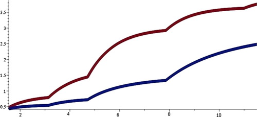This result can be visualized in Figure . If we impose the initial conditions $u (\frac{π}{4}) = v (\frac{π}{4}) = 0, u^{'} (\frac{π}{4}) = v^{'} (\frac{π}{4}) = 1$ to the system (Equation21(21) $\begin{aligned} - {(e^{t} u^{'})}^{'} - {(t^{2} u^{'})}^{'} = \sin t sgn (u) |v|, t \neq \frac{i π}{2}, \\ - {((t + 1) v^{'})}^{'} - {(t^{4} v^{'})}^{'} = \cos t sgn (v) |u|, t \neq \frac{i π}{2}, \\ {- Δ ((e^{t} + t^{2}) u^{'})|}_{t = \frac{i π}{2}} = \frac{(- 1)^{i}}{i} sgn (u) |v|, i \in N, \\ {- Δ ((t^{4} + t + 1) v^{'})|}_{t = \frac{i π}{2}} \\ = \frac{(- 1)^{i + 1}}{i} sgn (v) |u|, i \in N . \end{aligned}$ (21) ), the numerical solution of system (Equation21(21) $\begin{aligned} - {(e^{t} u^{'})}^{'} - {(t^{2} u^{'})}^{'} = \sin t sgn (u) |v|, t \neq \frac{i π}{2}, \\ - {((t + 1) v^{'})}^{'} - {(t^{4} v^{'})}^{'} = \cos t sgn (v) |u|, t \neq \frac{i π}{2}, \\ {- Δ ((e^{t} + t^{2}) u^{'})|}_{t = \frac{i π}{2}} = \frac{(- 1)^{i}}{i} sgn (u) |v|, i \in N, \\ {- Δ ((t^{4} + t + 1) v^{'})|}_{t = \frac{i π}{2}} \\ = \frac{(- 1)^{i + 1}}{i} sgn (v) |u|, i \in N . \end{aligned}$ (21) ) can be shown as in Figure . In this figure, the red and blue curves represent the solutions u and v, respectively. These solutions have zeros only at $t = \frac{π}{4}$ and they are different than zero when $t > \frac{π}{4} .$ Therefore, the solution $w (t) = (u (t), v (t))$ of system (Equation21(21) $\begin{aligned} - {(e^{t} u^{'})}^{'} - {(t^{2} u^{'})}^{'} = \sin t sgn (u) |v|, t \neq \frac{i π}{2}, \\ - {((t + 1) v^{'})}^{'} - {(t^{4} v^{'})}^{'} = \cos t sgn (v) |u|, t \neq \frac{i π}{2}, \\ {- Δ ((e^{t} + t^{2}) u^{'})|}_{t = \frac{i π}{2}} = \frac{(- 1)^{i}}{i} sgn (u) |v|, i \in N, \\ {- Δ ((t^{4} + t + 1) v^{'})|}_{t = \frac{i π}{2}} \\ = \frac{(- 1)^{i + 1}}{i} sgn (v) |u|, i \in N . \end{aligned}$ (21) ) can not be zero when $t > \frac{π}{4} .$ This implies that solution $w (t) = (u (t), v (t))$ of system (Equation21(21) $\begin{aligned} - {(e^{t} u^{'})}^{'} - {(t^{2} u^{'})}^{'} = \sin t sgn (u) |v|, t \neq \frac{i π}{2}, \\ - {((t + 1) v^{'})}^{'} - {(t^{4} v^{'})}^{'} = \cos t sgn (v) |u|, t \neq \frac{i π}{2}, \\ {- Δ ((e^{t} + t^{2}) u^{'})|}_{t = \frac{i π}{2}} = \frac{(- 1)^{i}}{i} sgn (u) |v|, i \in N, \\ {- Δ ((t^{4} + t + 1) v^{'})|}_{t = \frac{i π}{2}} \\ = \frac{(- 1)^{i + 1}}{i} sgn (v) |u|, i \in N . \end{aligned}$ (21) ) is disconjugate on $[\frac{π}{4}, 4 π]$ . Since the solution $w (t) = (u (t), v (t))$ is continuous at all points in $[\frac{π}{4}, 4 π]$ but its derivative has jumps at the jump points $τ_{i} = \frac{i π}{2}, i \in N,$ the edges on the graph of solution $w (t) = (u (t), v (t))$ occur at the impulse points $τ_{i} = \frac{i π}{2}, i \in N .$

2.2. Eigenvalue problems

Now, we present an application of the obtained Lyapunov-type inequality for system (Equation1(1) $\begin{aligned} - {(h_{1} (t) {|u^{'}|}^{p_{1} - 2} u^{'})}^{'} - {(m_{1} (t) {|u^{'}|}^{q_{1} - 2} u^{'})}^{'} \\ = f (t) {|u|}^{α - 2} u {|v|}^{β}, t \neq τ_{i} \\ - {(h_{2} (t) {|v^{'}|}^{p_{2} - 2} v^{'})}^{'} - {(m_{2} (t) {|v^{'}|}^{q_{2} - 2} v^{'})}^{'} \\ = g (t) {|u|}^{θ} {|v|}^{γ - 2} v, t \neq τ_{i} \\ {- Δ (h_{1} (t) {|u^{'}|}^{p_{1} - 2} u^{'} + m_{1} (t) {|u^{'}|}^{q_{1} - 2} u^{'})|}_{t = τ_{i}} \\ = a_{i} {|u|}^{α - 2} u {|v|}^{β}, i \in N, \\ {- Δ (h_{2} (t) {|v^{'}|}^{p_{2} - 2} v^{'} + m_{2} (t) {|v^{'}|}^{q_{2} - 2} v^{'})|}_{t = τ_{i}} \\ = b_{i} {|u|}^{θ} {|v|}^{γ - 2} v, i \in N . \end{aligned}$ (1) ). By using techniques similar to the technique in Napoli and Pinasco [Citation10], we establish the following result which gives lower bounds for eigenvalues of the associated eigenvalue problem of system (Equation1(1) $\begin{aligned} - {(h_{1} (t) {|u^{'}|}^{p_{1} - 2} u^{'})}^{'} - {(m_{1} (t) {|u^{'}|}^{q_{1} - 2} u^{'})}^{'} \\ = f (t) {|u|}^{α - 2} u {|v|}^{β}, t \neq τ_{i} \\ - {(h_{2} (t) {|v^{'}|}^{p_{2} - 2} v^{'})}^{'} - {(m_{2} (t) {|v^{'}|}^{q_{2} - 2} v^{'})}^{'} \\ = g (t) {|u|}^{θ} {|v|}^{γ - 2} v, t \neq τ_{i} \\ {- Δ (h_{1} (t) {|u^{'}|}^{p_{1} - 2} u^{'} + m_{1} (t) {|u^{'}|}^{q_{1} - 2} u^{'})|}_{t = τ_{i}} \\ = a_{i} {|u|}^{α - 2} u {|v|}^{β}, i \in N, \\ {- Δ (h_{2} (t) {|v^{'}|}^{p_{2} - 2} v^{'} + m_{2} (t) {|v^{'}|}^{q_{2} - 2} v^{'})|}_{t = τ_{i}} \\ = b_{i} {|u|}^{θ} {|v|}^{γ - 2} v, i \in N . \end{aligned}$ (1) ). The proof of the following theorem is based on the Lyapunov type inequality derived in Theorem 1.11.

Figure 1. The graph of solutions $u (t)$ and $v (t)$ of system (21).

Let $f (t) = λ α r_{1} (t)$ , $g (t) = μ β r_{2} (t)$ , $a_{i} = λ α c_{i 1}$ and $b_{i} = μ β c_{i 2},$ where $r_{1}, r_{2} > 0$ and $c_{i k} > 0, k = 1, 2$ . Then system (Equation1(1) $\begin{aligned} - {(h_{1} (t) {|u^{'}|}^{p_{1} - 2} u^{'})}^{'} - {(m_{1} (t) {|u^{'}|}^{q_{1} - 2} u^{'})}^{'} \\ = f (t) {|u|}^{α - 2} u {|v|}^{β}, t \neq τ_{i} \\ - {(h_{2} (t) {|v^{'}|}^{p_{2} - 2} v^{'})}^{'} - {(m_{2} (t) {|v^{'}|}^{q_{2} - 2} v^{'})}^{'} \\ = g (t) {|u|}^{θ} {|v|}^{γ - 2} v, t \neq τ_{i} \\ {- Δ (h_{1} (t) {|u^{'}|}^{p_{1} - 2} u^{'} + m_{1} (t) {|u^{'}|}^{q_{1} - 2} u^{'})|}_{t = τ_{i}} \\ = a_{i} {|u|}^{α - 2} u {|v|}^{β}, i \in N, \\ {- Δ (h_{2} (t) {|v^{'}|}^{p_{2} - 2} v^{'} + m_{2} (t) {|v^{'}|}^{q_{2} - 2} v^{'})|}_{t = τ_{i}} \\ = b_{i} {|u|}^{θ} {|v|}^{γ - 2} v, i \in N . \end{aligned}$ (1) ) reduces to the following impulsive eigenvalue problem (22) $\begin{aligned} \begin{array}{ll} - {(h_{1} (t) {|u^{'}|}^{p_{1} - 2} u^{'})}^{'} - {(m_{1} (t) {|u^{'}|}^{q_{1} - 2} u^{'})}^{'} \\ = λ α r_{1} (t) {|u|}^{α - 2} u {|v|}^{β}, & t \neq τ_{i} \\ - {(h_{2} (t) {|v^{'}|}^{p_{2} - 2} v^{'})}^{'} - {(m_{2} (t) {|v^{'}|}^{q_{2} - 2} v^{'})}^{'} \\ = μ β r_{2} (t) {|u|}^{θ} {|v|}^{γ - 2} v, & t \neq τ_{i} \\ {- Δ (h_{1} (t) {|u^{'}|}^{p_{1} - 2} u^{'} - m_{1} (t) {|u^{'}|}^{q_{1} - 2} u^{'})|}_{t = τ_{i}} \\ = λ α c_{i 1} {|u|}^{α - 2} u {|v|}^{β}, i = 1, 2, \dots, m \\ {- Δ (h_{2} (t) {|v^{'}|}^{p_{2} - 2} v^{'} - m_{2} (t) {|v^{'}|}^{q_{2} - 2} v^{'})|}_{t = τ_{i}} \\ = μ β c_{i 2} {|u|}^{θ} {|v|}^{γ - 2} v, i = 1, 2, \dots, m \\ u (a) = u (b) = v (a) = v (b) = 0. \end{array} \end{aligned}$ (22)

Definition 2.3

A pair $(λ, μ)$ is called an eigenvalue of (Equation22(22) $\begin{aligned} \begin{array}{ll} - {(h_{1} (t) {|u^{'}|}^{p_{1} - 2} u^{'})}^{'} - {(m_{1} (t) {|u^{'}|}^{q_{1} - 2} u^{'})}^{'} \\ = λ α r_{1} (t) {|u|}^{α - 2} u {|v|}^{β}, & t \neq τ_{i} \\ - {(h_{2} (t) {|v^{'}|}^{p_{2} - 2} v^{'})}^{'} - {(m_{2} (t) {|v^{'}|}^{q_{2} - 2} v^{'})}^{'} \\ = μ β r_{2} (t) {|u|}^{θ} {|v|}^{γ - 2} v, & t \neq τ_{i} \\ {- Δ (h_{1} (t) {|u^{'}|}^{p_{1} - 2} u^{'} - m_{1} (t) {|u^{'}|}^{q_{1} - 2} u^{'})|}_{t = τ_{i}} \\ = λ α c_{i 1} {|u|}^{α - 2} u {|v|}^{β}, i = 1, 2, \dots, m \\ {- Δ (h_{2} (t) {|v^{'}|}^{p_{2} - 2} v^{'} - m_{2} (t) {|v^{'}|}^{q_{2} - 2} v^{'})|}_{t = τ_{i}} \\ = μ β c_{i 2} {|u|}^{θ} {|v|}^{γ - 2} v, i = 1, 2, \dots, m \\ u (a) = u (b) = v (a) = v (b) = 0. \end{array} \end{aligned}$ (22) ) if there is a corresponding solution $(u, v)$ such that $u, v ≢ 0$ on $(a, b)$ .

Theorem 2.4

Assume that the condition (Equation3(3) $\begin{aligned} \frac{2 α}{p_{1} + q_{1}} + \frac{2 β}{p_{2} + q_{2}} = 1 \\ and \frac{2 θ}{p_{1} + q_{1}} + \frac{2 γ}{p_{2} + q_{2}} = 1. \end{aligned}$ (3) ) holds. Let $p_{j}^{'}$ and $q_{j}^{'}$ be conjugate numbers for $p_{j}$ and $q_{j}$ , $j = 1, 2,$ respectively and $(e_{1}, e_{2})$ be a nontrivial solution of the homogenous system (Equation4(4) $\begin{aligned} e_{1} (α - \frac{p_{1} + q_{1}}{2}) + e_{2} θ = 0, \\ e_{1} β + e_{2} (γ - \frac{p_{2} + q_{2}}{2}) = 0, \end{aligned}$ (4) ) and (23) $\int_{a}^{b} r_{k} (t) d t + \sum_{a \leq τ_{i} < b} c_{i k} > 0, k = 1, 2.$ (23) Then there exists a function $h (λ) = \frac{1}{β} (\frac{C D}{(| λ | α)^{e_{1}}})^{\frac{1}{e_{2}}}$ such that $| μ | \geq h (λ)$ for every eigenvalue pair $(λ, μ)$ of the system (Equation22(22) $\begin{aligned} \begin{array}{ll} - {(h_{1} (t) {|u^{'}|}^{p_{1} - 2} u^{'})}^{'} - {(m_{1} (t) {|u^{'}|}^{q_{1} - 2} u^{'})}^{'} \\ = λ α r_{1} (t) {|u|}^{α - 2} u {|v|}^{β}, & t \neq τ_{i} \\ - {(h_{2} (t) {|v^{'}|}^{p_{2} - 2} v^{'})}^{'} - {(m_{2} (t) {|v^{'}|}^{q_{2} - 2} v^{'})}^{'} \\ = μ β r_{2} (t) {|u|}^{θ} {|v|}^{γ - 2} v, & t \neq τ_{i} \\ {- Δ (h_{1} (t) {|u^{'}|}^{p_{1} - 2} u^{'} - m_{1} (t) {|u^{'}|}^{q_{1} - 2} u^{'})|}_{t = τ_{i}} \\ = λ α c_{i 1} {|u|}^{α - 2} u {|v|}^{β}, i = 1, 2, \dots, m \\ {- Δ (h_{2} (t) {|v^{'}|}^{p_{2} - 2} v^{'} - m_{2} (t) {|v^{'}|}^{q_{2} - 2} v^{'})|}_{t = τ_{i}} \\ = μ β c_{i 2} {|u|}^{θ} {|v|}^{γ - 2} v, i = 1, 2, \dots, m \\ u (a) = u (b) = v (a) = v (b) = 0. \end{array} \end{aligned}$ (22) ) where the constants C and D are given as $\begin{aligned} C & = 2^{e_{1} + e_{2}} {[min \{2^{p_{1}} N (b, h_{1}, p_{1}), 2^{q_{1}} N (b, m_{1}, q_{1})\}]}^{e_{1}} \\ \times {[min \{2^{p_{2}} N (b, h_{2}, p_{2}), 2^{q_{2}} N (b, m_{2}, q_{2})\}]}^{e_{2}}, \\ D & = {(\int_{a}^{b} r_{1} (t) d t + \sum_{a \leq τ_{i} < b} c_{i 1})}^{- e_{1}} \\ \times {(\int_{a}^{b} r_{2} (t) d t + \sum_{a \leq τ_{i} < b} c_{i 1})}^{- e_{2}} . \end{aligned}$

Proof.

Let $(λ, μ)$ be an eigenvalue pair and $(u, v)$ be the corresponding eigenfunctions of the system (Equation22(22) $\begin{aligned} \begin{array}{ll} - {(h_{1} (t) {|u^{'}|}^{p_{1} - 2} u^{'})}^{'} - {(m_{1} (t) {|u^{'}|}^{q_{1} - 2} u^{'})}^{'} \\ = λ α r_{1} (t) {|u|}^{α - 2} u {|v|}^{β}, & t \neq τ_{i} \\ - {(h_{2} (t) {|v^{'}|}^{p_{2} - 2} v^{'})}^{'} - {(m_{2} (t) {|v^{'}|}^{q_{2} - 2} v^{'})}^{'} \\ = μ β r_{2} (t) {|u|}^{θ} {|v|}^{γ - 2} v, & t \neq τ_{i} \\ {- Δ (h_{1} (t) {|u^{'}|}^{p_{1} - 2} u^{'} - m_{1} (t) {|u^{'}|}^{q_{1} - 2} u^{'})|}_{t = τ_{i}} \\ = λ α c_{i 1} {|u|}^{α - 2} u {|v|}^{β}, i = 1, 2, \dots, m \\ {- Δ (h_{2} (t) {|v^{'}|}^{p_{2} - 2} v^{'} - m_{2} (t) {|v^{'}|}^{q_{2} - 2} v^{'})|}_{t = τ_{i}} \\ = μ β c_{i 2} {|u|}^{θ} {|v|}^{γ - 2} v, i = 1, 2, \dots, m \\ u (a) = u (b) = v (a) = v (b) = 0. \end{array} \end{aligned}$ (22) ). If we apply Lyapunov inequality obtained in Theorem 1.11 for system (Equation22(22) $\begin{aligned} \begin{array}{ll} - {(h_{1} (t) {|u^{'}|}^{p_{1} - 2} u^{'})}^{'} - {(m_{1} (t) {|u^{'}|}^{q_{1} - 2} u^{'})}^{'} \\ = λ α r_{1} (t) {|u|}^{α - 2} u {|v|}^{β}, & t \neq τ_{i} \\ - {(h_{2} (t) {|v^{'}|}^{p_{2} - 2} v^{'})}^{'} - {(m_{2} (t) {|v^{'}|}^{q_{2} - 2} v^{'})}^{'} \\ = μ β r_{2} (t) {|u|}^{θ} {|v|}^{γ - 2} v, & t \neq τ_{i} \\ {- Δ (h_{1} (t) {|u^{'}|}^{p_{1} - 2} u^{'} - m_{1} (t) {|u^{'}|}^{q_{1} - 2} u^{'})|}_{t = τ_{i}} \\ = λ α c_{i 1} {|u|}^{α - 2} u {|v|}^{β}, i = 1, 2, \dots, m \\ {- Δ (h_{2} (t) {|v^{'}|}^{p_{2} - 2} v^{'} - m_{2} (t) {|v^{'}|}^{q_{2} - 2} v^{'})|}_{t = τ_{i}} \\ = μ β c_{i 2} {|u|}^{θ} {|v|}^{γ - 2} v, i = 1, 2, \dots, m \\ u (a) = u (b) = v (a) = v (b) = 0. \end{array} \end{aligned}$ (22) ), we get (24) $\begin{aligned} C & \leq {(\int_{a}^{b} | λ | α r_{1} (t) d t + \sum_{a \leq τ_{i} < b} | λ | α c_{i 1})}^{e_{1}} \\ \times {(\int_{a}^{b} | μ | β r_{2} (t) d t + \sum_{a \leq τ_{i} < b} | μ | β c_{i 2})}^{e_{2}} \\ = {(\int_{a}^{b} r_{1} (t) d t + \sum_{a \leq τ_{i} < b} c_{i 1})}^{e_{1}} \\ \times {(\int_{a}^{b} r_{2} (t) d t + \sum_{a \leq τ_{i} < b} c_{i 2})}^{e_{2}} (| λ | α)^{e_{1}} (| μ | β)^{e_{2}} . \end{aligned}$ (24) For the eigenvalue μ, we can find the following lower bound as $\begin{aligned} | μ | β & \geq C^{\frac{1}{e_{2}}} (| λ | α)^{\frac{- e_{1}}{e_{2}}} {(\int_{a}^{b} r_{1} (t) d t + \sum_{a \leq τ_{i} < b} c_{i 1})}^{\frac{- e_{1}}{e_{2}}} \\ \times {(\int_{a}^{b} r_{2} (t) d t + \sum_{a \leq τ_{i} < b} c_{i 2})}^{- 1} . \end{aligned}$ Also by rearranging terms in (Equation24(24) $\begin{aligned} C & \leq {(\int_{a}^{b} | λ | α r_{1} (t) d t + \sum_{a \leq τ_{i} < b} | λ | α c_{i 1})}^{e_{1}} \\ \times {(\int_{a}^{b} | μ | β r_{2} (t) d t + \sum_{a \leq τ_{i} < b} | μ | β c_{i 2})}^{e_{2}} \\ = {(\int_{a}^{b} r_{1} (t) d t + \sum_{a \leq τ_{i} < b} c_{i 1})}^{e_{1}} \\ \times {(\int_{a}^{b} r_{2} (t) d t + \sum_{a \leq τ_{i} < b} c_{i 2})}^{e_{2}} (| λ | α)^{e_{1}} (| μ | β)^{e_{2}} . \end{aligned}$ (24) ), we obtain $| λ |^{e_{1}} | μ |^{e_{2}} \geq \frac{C D}{α^{e_{1}} β^{e_{2}}} .$

Since the proofs of following corollaries are the same as that of Theorem 2.4, they are omitted.

Corollary 2.5

Assume that the condition (Equation3(3) $\begin{aligned} \frac{2 α}{p_{1} + q_{1}} + \frac{2 β}{p_{2} + q_{2}} = 1 \\ and \frac{2 θ}{p_{1} + q_{1}} + \frac{2 γ}{p_{2} + q_{2}} = 1. \end{aligned}$ (3) ) holds. Let $p_{j}^{'}$ and $q_{j}^{'}$ be conjugate numbers for $p_{j}$ and $q_{j}, j = 1, 2$ , respectively. Suppose that (Equation17(17) $α + θ = \frac{p_{1} + q_{1}}{2}, β + γ = \frac{p_{2} + q_{2}}{2} .$ (17) ) and (Equation23(23) $\int_{a}^{b} r_{k} (t) d t + \sum_{a \leq τ_{i} < b} c_{i k} > 0, k = 1, 2.$ (23) ) hold. Then there exists a function $h_{1} (λ) = \frac{1}{β} (\frac{C_{1} D_{1}}{| λ | α})$ such that $| μ | \geq h_{1} (λ)$ for every eigenvalue pair $(λ, μ)$ of the system (Equation22(22) $\begin{aligned} \begin{array}{ll} - {(h_{1} (t) {|u^{'}|}^{p_{1} - 2} u^{'})}^{'} - {(m_{1} (t) {|u^{'}|}^{q_{1} - 2} u^{'})}^{'} \\ = λ α r_{1} (t) {|u|}^{α - 2} u {|v|}^{β}, & t \neq τ_{i} \\ - {(h_{2} (t) {|v^{'}|}^{p_{2} - 2} v^{'})}^{'} - {(m_{2} (t) {|v^{'}|}^{q_{2} - 2} v^{'})}^{'} \\ = μ β r_{2} (t) {|u|}^{θ} {|v|}^{γ - 2} v, & t \neq τ_{i} \\ {- Δ (h_{1} (t) {|u^{'}|}^{p_{1} - 2} u^{'} - m_{1} (t) {|u^{'}|}^{q_{1} - 2} u^{'})|}_{t = τ_{i}} \\ = λ α c_{i 1} {|u|}^{α - 2} u {|v|}^{β}, i = 1, 2, \dots, m \\ {- Δ (h_{2} (t) {|v^{'}|}^{p_{2} - 2} v^{'} - m_{2} (t) {|v^{'}|}^{q_{2} - 2} v^{'})|}_{t = τ_{i}} \\ = μ β c_{i 2} {|u|}^{θ} {|v|}^{γ - 2} v, i = 1, 2, \dots, m \\ u (a) = u (b) = v (a) = v (b) = 0. \end{array} \end{aligned}$ (22) ) where the constants $C_{1}$ and $D_{1}$ are given as $\begin{aligned} C_{1} & = 2^{2} [min \{2^{p_{1}} N (b, h_{1}, p_{1}), 2^{q_{1}} N (b, m_{1}, q_{1})\}] \\ \times [min \{2^{p_{2}} N (b, h_{2}, p_{2}), 2^{q_{2}} N (b, m_{2}, q_{2})\}], \\ D_{1} & = {(\int_{a}^{b} r_{1} (t) d t + \sum_{a \leq τ_{i} < b} c_{i 1})}^{- 1} \\ \times {(\int_{a}^{b} r_{2} (t) d t + \sum_{a \leq τ_{i} < b} c_{i 1})}^{- 1} . \end{aligned}$

Corollary 2.6

Assume that the condition (Equation3(3) $\begin{aligned} \frac{2 α}{p_{1} + q_{1}} + \frac{2 β}{p_{2} + q_{2}} = 1 \\ and \frac{2 θ}{p_{1} + q_{1}} + \frac{2 γ}{p_{2} + q_{2}} = 1. \end{aligned}$ (3) ) holds. Let $p_{j}^{'}$ and $q_{j}^{'}$ be conjugate numbers for $p_{j}$ and $q_{j}, j = 1, 2$ , respectively. Suppose that (Equation18(18) $\frac{2 α}{p_{1} + q_{1}} + \frac{2 γ}{p_{2} + q_{2}} = 1, β θ = α γ .$ (18) ) and (Equation23(23) $\int_{a}^{b} r_{k} (t) d t + \sum_{a \leq τ_{i} < b} c_{i k} > 0, k = 1, 2.$ (23) ) hold. Then there exists a function $h_{2} (λ) = \frac{1}{β} {(\frac{C_{2} D_{2}}{(| λ | α)^{θ}})}^{\frac{2}{p_{1} + q_{1} - 2 α}}$ such that $| μ | \geq h_{2} (λ)$ for every eigenvalue pair $(λ, μ)$ of the system (Equation22(22) $\begin{aligned} \begin{array}{ll} - {(h_{1} (t) {|u^{'}|}^{p_{1} - 2} u^{'})}^{'} - {(m_{1} (t) {|u^{'}|}^{q_{1} - 2} u^{'})}^{'} \\ = λ α r_{1} (t) {|u|}^{α - 2} u {|v|}^{β}, & t \neq τ_{i} \\ - {(h_{2} (t) {|v^{'}|}^{p_{2} - 2} v^{'})}^{'} - {(m_{2} (t) {|v^{'}|}^{q_{2} - 2} v^{'})}^{'} \\ = μ β r_{2} (t) {|u|}^{θ} {|v|}^{γ - 2} v, & t \neq τ_{i} \\ {- Δ (h_{1} (t) {|u^{'}|}^{p_{1} - 2} u^{'} - m_{1} (t) {|u^{'}|}^{q_{1} - 2} u^{'})|}_{t = τ_{i}} \\ = λ α c_{i 1} {|u|}^{α - 2} u {|v|}^{β}, i = 1, 2, \dots, m \\ {- Δ (h_{2} (t) {|v^{'}|}^{p_{2} - 2} v^{'} - m_{2} (t) {|v^{'}|}^{q_{2} - 2} v^{'})|}_{t = τ_{i}} \\ = μ β c_{i 2} {|u|}^{θ} {|v|}^{γ - 2} v, i = 1, 2, \dots, m \\ u (a) = u (b) = v (a) = v (b) = 0. \end{array} \end{aligned}$ (22) ) where the constants $C_{2}$ and $D_{2}$ are given as $\begin{aligned} C_{2} & = 2^{\frac{p_{1} + q_{1}}{2} - α + θ} \\ \times {[min \{2^{p_{1}} N (b, h_{1}, p_{1}), 2^{q_{1}} N (b, m_{1}, q_{1})\}]}^{θ} \\ \times {[min \{2^{p_{2}} N (b, h_{2}, p_{2}), 2^{q_{2}} N (b, m_{2}, q_{2})\}]}^{\frac{p_{1} + q_{1}}{2} - α}, \\ D_{2} & = {(\int_{a}^{b} r_{1} (t) d t + \sum_{a \leq τ_{i} < b} c_{i 1})}^{- θ} \\ \times {(\int_{a}^{b} r_{2} (t) d t + \sum_{a \leq τ_{i} < b} c_{i 1})}^{α - \frac{p_{1} + q_{1}}{2}} . \end{aligned}$

Corollary 2.7

Assume that the condition (Equation3(3) $\begin{aligned} \frac{2 α}{p_{1} + q_{1}} + \frac{2 β}{p_{2} + q_{2}} = 1 \\ and \frac{2 θ}{p_{1} + q_{1}} + \frac{2 γ}{p_{2} + q_{2}} = 1. \end{aligned}$ (3) ) holds. Let $p_{j}^{'}$ and $q_{j}^{'}$ be conjugate numbers for $p_{j}$ and $q_{j}, j = 1, 2$ , respectively, $α = θ$ and $β = γ$ and $(e_{1}, e_{2})$ be a nontrivial solution of the homogenous system (Equation19(19) $\begin{aligned} e_{1} (α - \frac{p_{1} + q_{1}}{2}) + e_{2} α = 0, \\ e_{1} β + e_{2} (β - \frac{p_{2} + q_{2}}{2}) = 0, \end{aligned}$ (19) ). Suppose that (Equation23(23) $\int_{a}^{b} r_{k} (t) d t + \sum_{a \leq τ_{i} < b} c_{i k} > 0, k = 1, 2.$ (23) ) holds. Then there exists a function $h_{3} (λ) = \frac{1}{β} {(\frac{C_{3} D_{3}}{(| λ | α)^{e_{1}}})}^{\frac{1}{e_{2}}}$ such that $| μ | \geq h_{3} (λ)$ for every eigenvalue pair $(λ, μ)$ of the system (Equation22(22) $\begin{aligned} \begin{array}{ll} - {(h_{1} (t) {|u^{'}|}^{p_{1} - 2} u^{'})}^{'} - {(m_{1} (t) {|u^{'}|}^{q_{1} - 2} u^{'})}^{'} \\ = λ α r_{1} (t) {|u|}^{α - 2} u {|v|}^{β}, & t \neq τ_{i} \\ - {(h_{2} (t) {|v^{'}|}^{p_{2} - 2} v^{'})}^{'} - {(m_{2} (t) {|v^{'}|}^{q_{2} - 2} v^{'})}^{'} \\ = μ β r_{2} (t) {|u|}^{θ} {|v|}^{γ - 2} v, & t \neq τ_{i} \\ {- Δ (h_{1} (t) {|u^{'}|}^{p_{1} - 2} u^{'} - m_{1} (t) {|u^{'}|}^{q_{1} - 2} u^{'})|}_{t = τ_{i}} \\ = λ α c_{i 1} {|u|}^{α - 2} u {|v|}^{β}, i = 1, 2, \dots, m \\ {- Δ (h_{2} (t) {|v^{'}|}^{p_{2} - 2} v^{'} - m_{2} (t) {|v^{'}|}^{q_{2} - 2} v^{'})|}_{t = τ_{i}} \\ = μ β c_{i 2} {|u|}^{θ} {|v|}^{γ - 2} v, i = 1, 2, \dots, m \\ u (a) = u (b) = v (a) = v (b) = 0. \end{array} \end{aligned}$ (22) ) where the constants $C_{3}$ and $D_{3}$ are given as $\begin{aligned} C_{3} & = 2^{e_{1} + e_{2}} {[min \{2^{p_{1}} N (b, h_{1}, p_{1}), 2^{q_{1}} N (b, m_{1}, q_{1})\}]}^{e_{1}} \\ \times {[min \{2^{p_{2}} N (b, h_{2}, p_{2}), 2^{q_{2}} N (b, m_{2}, q_{2})\}]}^{e_{2}}, \\ D_{3} & = {(\int_{a}^{b} r_{1} (t) d t + \sum_{a \leq τ_{i} < b} c_{i 1})}^{- e_{1}} \\ \times {(\int_{a}^{b} r_{2} (t) d t + \sum_{a \leq τ_{i} < b} c_{i 1})}^{- e_{2}} . \end{aligned}$

2.3. Asymptotic behaviour of oscillatory solutions

In this section as an application of Lyapunov type inequality given in Section 1.1, we establish the following results to study the asymptotic behaviour of the oscillatory solutions of system (Equation1(1) $\begin{aligned} - {(h_{1} (t) {|u^{'}|}^{p_{1} - 2} u^{'})}^{'} - {(m_{1} (t) {|u^{'}|}^{q_{1} - 2} u^{'})}^{'} \\ = f (t) {|u|}^{α - 2} u {|v|}^{β}, t \neq τ_{i} \\ - {(h_{2} (t) {|v^{'}|}^{p_{2} - 2} v^{'})}^{'} - {(m_{2} (t) {|v^{'}|}^{q_{2} - 2} v^{'})}^{'} \\ = g (t) {|u|}^{θ} {|v|}^{γ - 2} v, t \neq τ_{i} \\ {- Δ (h_{1} (t) {|u^{'}|}^{p_{1} - 2} u^{'} + m_{1} (t) {|u^{'}|}^{q_{1} - 2} u^{'})|}_{t = τ_{i}} \\ = a_{i} {|u|}^{α - 2} u {|v|}^{β}, i \in N, \\ {- Δ (h_{2} (t) {|v^{'}|}^{p_{2} - 2} v^{'} + m_{2} (t) {|v^{'}|}^{q_{2} - 2} v^{'})|}_{t = τ_{i}} \\ = b_{i} {|u|}^{θ} {|v|}^{γ - 2} v, i \in N . \end{aligned}$ (1) ).

Theorem 2.8

Assume that the condition (Equation3(3) $\begin{aligned} \frac{2 α}{p_{1} + q_{1}} + \frac{2 β}{p_{2} + q_{2}} = 1 \\ and \frac{2 θ}{p_{1} + q_{1}} + \frac{2 γ}{p_{2} + q_{2}} = 1. \end{aligned}$ (3) ) holds. Let $p_{j}^{'}$ and $q_{j}^{'}$ be conjugate numbers for $p_{j}$ and $q_{j}$ , $j = 1, 2,$ respectively and $(e_{1}, e_{2})$ be a nontrivial solution of the homogenous system (Equation4(4) $\begin{aligned} e_{1} (α - \frac{p_{1} + q_{1}}{2}) + e_{2} θ = 0, \\ e_{1} β + e_{2} (γ - \frac{p_{2} + q_{2}}{2}) = 0, \end{aligned}$ (4) ). Let $\begin{aligned} {(\int^{\infty} f^{+} (t) d t + \sum_{τ_{i} < \infty} a_{i}^{+})}^{e_{1}} \\ \times {(\int^{\infty} g^{+} (t) d t + \sum_{τ_{i} < \infty} b_{i}^{+})}^{e_{2}} \\ \times {[min \{2^{p_{1}} N (\infty, h_{1}, p_{1}), 2^{q_{1}} N (\infty, m_{1}, q_{1})\}]}^{- e_{1}} \\ \times {[min \{2^{p_{2}} N (\infty, h_{2}, p_{2}), 2^{q_{2}} N (\infty, m_{2}, q_{2})\}]}^{- e_{2}} < \infty, \end{aligned}$ where $N (\infty, k, μ) = {(\int^{\infty} (k (t))^{\frac{- μ^{'}}{μ}} d t)}^{1 - μ} .$ Then every oscillatory solution $w (t) = (u (t), v (t))$ of system (Equation1(1) $\begin{aligned} - {(h_{1} (t) {|u^{'}|}^{p_{1} - 2} u^{'})}^{'} - {(m_{1} (t) {|u^{'}|}^{q_{1} - 2} u^{'})}^{'} \\ = f (t) {|u|}^{α - 2} u {|v|}^{β}, t \neq τ_{i} \\ - {(h_{2} (t) {|v^{'}|}^{p_{2} - 2} v^{'})}^{'} - {(m_{2} (t) {|v^{'}|}^{q_{2} - 2} v^{'})}^{'} \\ = g (t) {|u|}^{θ} {|v|}^{γ - 2} v, t \neq τ_{i} \\ {- Δ (h_{1} (t) {|u^{'}|}^{p_{1} - 2} u^{'} + m_{1} (t) {|u^{'}|}^{q_{1} - 2} u^{'})|}_{t = τ_{i}} \\ = a_{i} {|u|}^{α - 2} u {|v|}^{β}, i \in N, \\ {- Δ (h_{2} (t) {|v^{'}|}^{p_{2} - 2} v^{'} + m_{2} (t) {|v^{'}|}^{q_{2} - 2} v^{'})|}_{t = τ_{i}} \\ = b_{i} {|u|}^{θ} {|v|}^{γ - 2} v, i \in N . \end{aligned}$ (1) ) is bounded and approaches zero as $t \to \infty$ .

Proof.

First we prove the boundedness of oscillatory solution $w (t) = (u (t), v (t))$ . Let us suppose that $w (t)$ is oscillatory but not bounded. Then $\underset{t \to \infty}{lim sup} | w (t) | = \infty .$ Then for every $M_{1}$ , we can find $T = T (M_{1})$ such that $| w (t) | > M_{1}$ for all t>T. Since w is oscillatory, there exists an interval $(t_{1}, t_{2})$ with $t_{1} \geq T$ such that $w (t_{1}) = w (t_{2}) = 0$ . By using Lyapunov inequality for $t_{1} \geq T$ , we get $\begin{aligned} {(\int_{t_{1}}^{t_{2}} f^{+} (t) d t + \sum_{t_{1} \leq τ_{i} < t_{2}} a_{i}^{+})}^{e_{1}} \\ \times {(\int_{t_{1}}^{t_{2}} g^{+} (t) d t + \sum_{t_{1} \leq τ_{i} < t_{2}} b_{i}^{+})}^{e_{2}} \\ \geq 2^{e_{1} + e_{2}} {[min \{2^{p_{1}} N (t_{2}, h_{1}, p_{1}), 2^{q_{1}} N (t_{2}, m_{1}, q_{1})\}]}^{e_{1}} \\ \times {[min \{2^{p_{2}} N (t_{2}, h_{2}, p_{2}), 2^{q_{2}} N (t_{2}, m_{2}, q_{2})\}]}^{e_{2}} . \end{aligned}$ Since $N (s, k, μ) \leq N (t_{2}, k, μ)$ for $s \geq t_{2},$ we obtain $\begin{aligned} {(\int_{a}^{s} f^{+} (t) d t + \sum_{a \leq τ_{i} < s} a_{i}^{+})}^{e_{1}} \\ \times {(\int_{a}^{s} g^{+} (t) d t + \sum_{a \leq τ_{i} < s} b_{i}^{+})}^{e_{2}} \\ \geq 2^{e_{1} + e_{2}} {[min \{2^{p_{1}} N (s, h_{1}, p_{1}), 2^{q_{1}} N (s, m_{1}, q_{1})\}]}^{e_{1}} \\ \times {[min \{2^{p_{2}} N (s, h_{2}, p_{2}), 2^{q_{2}} N (s, m_{2}, q_{2})\}]}^{e_{2}} \end{aligned}$ or $\begin{aligned} 2^{e_{1} + e_{2}} & \leq {(\int_{a}^{\infty} f^{+} (t) d t + \sum_{a \leq τ_{i} < \infty} a_{i}^{+})}^{e_{1}} \\ \times {(\int_{a}^{\infty} g^{+} (t) d t + \sum_{a \leq τ_{i} < \infty} b_{i}^{+})}^{e_{2}} \\ \times {[min \{2^{p_{1}} N (\infty, h_{1}, p_{1}), 2^{q_{1}} N (\infty, m_{1}, q_{1})\}]}^{- e_{1}} \\ \times {[min \{2^{p_{2}} N (\infty, h_{2}, p_{2}), 2^{q_{2}} N (\infty, m_{2}, q_{2})\}]}^{- e_{2}} \\ \leq 1, \end{aligned}$ where $N (\infty, k, μ) = (\int_{a}^{\infty} (k (t))^{\frac{- μ^{'}}{μ}} d t)^{1 - μ} .$ Then we get $e_{1} + e_{2} \leq 0$ which implies contradiction. Therefore, w is bounded. Since w is bounded, $| w (t) | \leq N$ for t>T for any T. If $w (t)$ does not approach zero as $t \to \infty$ , then there exists a constant d>0 such that $2 d \leq \underset{t \to \infty}{lim sup} | w (t) | \leq N .$ Since w has arbitrarily large zeros, there exists an interval $(t_{1}, t_{2})$ with $t_{1} \geq T$ , where T is sufficiently large, such that $w (t_{1}) = w (t_{2}) = 0$ . The remainder of the proof is similar to above, hence it is omitted.

The following corollaries and their proofs follow easily from Theorem 2.8 and its proof, respectively.

Corollary 2.9

Assume that the condition (Equation3(3) $\begin{aligned} \frac{2 α}{p_{1} + q_{1}} + \frac{2 β}{p_{2} + q_{2}} = 1 \\ and \frac{2 θ}{p_{1} + q_{1}} + \frac{2 γ}{p_{2} + q_{2}} = 1. \end{aligned}$ (3) ) holds. Let $p_{j}^{'}$ and $q_{j}^{'}$ be conjugate numbers for $p_{j}$ and $q_{j}, j = 1, 2$ , respectively. Suppose that (Equation17(17) $α + θ = \frac{p_{1} + q_{1}}{2}, β + γ = \frac{p_{2} + q_{2}}{2} .$ (17) ) holds. Let $\begin{aligned} (\int^{\infty} f^{+} (t) d t + \sum_{τ_{i} < \infty} a_{i}^{+}) (\int^{\infty} g^{+} (t) d t + \sum_{τ_{i} < \infty} b_{i}^{+}) \\ \times {[min \{2^{p_{1}} N (\infty, h_{1}, p_{1}), 2^{q_{1}} N (\infty, m_{1}, q_{1})\}]}^{- 1} \\ \times {[min \{2^{p_{2}} N (\infty, h_{2}, p_{2}), 2^{q_{2}} N (\infty, m_{2}, q_{2})\}]}^{- 1} < \infty, \end{aligned}$ where $N (\infty, k, μ) = (\int^{\infty} {(k (t))^{\frac{- μ^{'}}{μ}} d t)}^{1 - μ} .$ Then every oscillatory solution $w (t) = (u (t), v (t))$ of system (Equation1(1) $\begin{aligned} - {(h_{1} (t) {|u^{'}|}^{p_{1} - 2} u^{'})}^{'} - {(m_{1} (t) {|u^{'}|}^{q_{1} - 2} u^{'})}^{'} \\ = f (t) {|u|}^{α - 2} u {|v|}^{β}, t \neq τ_{i} \\ - {(h_{2} (t) {|v^{'}|}^{p_{2} - 2} v^{'})}^{'} - {(m_{2} (t) {|v^{'}|}^{q_{2} - 2} v^{'})}^{'} \\ = g (t) {|u|}^{θ} {|v|}^{γ - 2} v, t \neq τ_{i} \\ {- Δ (h_{1} (t) {|u^{'}|}^{p_{1} - 2} u^{'} + m_{1} (t) {|u^{'}|}^{q_{1} - 2} u^{'})|}_{t = τ_{i}} \\ = a_{i} {|u|}^{α - 2} u {|v|}^{β}, i \in N, \\ {- Δ (h_{2} (t) {|v^{'}|}^{p_{2} - 2} v^{'} + m_{2} (t) {|v^{'}|}^{q_{2} - 2} v^{'})|}_{t = τ_{i}} \\ = b_{i} {|u|}^{θ} {|v|}^{γ - 2} v, i \in N . \end{aligned}$ (1) ) is bounded and approaches zero as $t \to \infty$ .

Corollary 2.10

Assume that the condition (Equation3(3) $\begin{aligned} \frac{2 α}{p_{1} + q_{1}} + \frac{2 β}{p_{2} + q_{2}} = 1 \\ and \frac{2 θ}{p_{1} + q_{1}} + \frac{2 γ}{p_{2} + q_{2}} = 1. \end{aligned}$ (3) ) holds. Let $p_{j}^{'}$ and $q_{j}^{'}$ be conjugate numbers for $p_{j}$ and $q_{j}, j = 1, 2,$ respectively. Suppose that (Equation18(18) $\frac{2 α}{p_{1} + q_{1}} + \frac{2 γ}{p_{2} + q_{2}} = 1, β θ = α γ .$ (18) ) holds. Let $\begin{aligned} {(\int^{\infty} f^{+} (t) d t + \sum_{τ_{i} < \infty} a_{i}^{+})}^{θ} \\ \times {(\int^{\infty} g^{+} (t) d t + \sum_{τ_{i} < \infty} b_{i}^{+})}^{\frac{p_{1} + q_{1}}{2} - α} \\ \times {[min \{2^{p_{1}} N (\infty, h_{1}, p_{1}), 2^{q_{1}} N (\infty, m_{1}, q_{1})\}]}^{- θ} \\ \times {[min \{2^{p_{2}} N (\infty, h_{2}, p_{2}), 2^{q_{2}} N (\infty, m_{2}, q_{2})\}]}^{α - \frac{p_{1} + q_{1}}{2}} \\ < \infty, \end{aligned}$ where $N (\infty, k, μ) = (\int^{\infty} (k (t))^{\frac{- μ^{'}}{μ}} d t)^{1 - μ} .$ Then every oscillatory solution $w (t) = (u (t), v (t))$ of system (Equation1(1) $\begin{aligned} - {(h_{1} (t) {|u^{'}|}^{p_{1} - 2} u^{'})}^{'} - {(m_{1} (t) {|u^{'}|}^{q_{1} - 2} u^{'})}^{'} \\ = f (t) {|u|}^{α - 2} u {|v|}^{β}, t \neq τ_{i} \\ - {(h_{2} (t) {|v^{'}|}^{p_{2} - 2} v^{'})}^{'} - {(m_{2} (t) {|v^{'}|}^{q_{2} - 2} v^{'})}^{'} \\ = g (t) {|u|}^{θ} {|v|}^{γ - 2} v, t \neq τ_{i} \\ {- Δ (h_{1} (t) {|u^{'}|}^{p_{1} - 2} u^{'} + m_{1} (t) {|u^{'}|}^{q_{1} - 2} u^{'})|}_{t = τ_{i}} \\ = a_{i} {|u|}^{α - 2} u {|v|}^{β}, i \in N, \\ {- Δ (h_{2} (t) {|v^{'}|}^{p_{2} - 2} v^{'} + m_{2} (t) {|v^{'}|}^{q_{2} - 2} v^{'})|}_{t = τ_{i}} \\ = b_{i} {|u|}^{θ} {|v|}^{γ - 2} v, i \in N . \end{aligned}$ (1) ) is bounded and approaches zero as $t \to \infty$ .

Corollary 2.11

Assume that the condition (Equation3(3) $\begin{aligned} \frac{2 α}{p_{1} + q_{1}} + \frac{2 β}{p_{2} + q_{2}} = 1 \\ and \frac{2 θ}{p_{1} + q_{1}} + \frac{2 γ}{p_{2} + q_{2}} = 1. \end{aligned}$ (3) ) holds. Let $p_{j}^{'}$ and $q_{j}^{'}$ be conjugate numbers for $p_{j}$ and $q_{j}, j = 1, 2$ , respectively, $α = θ$ and $β = γ$ and $(e_{1}, e_{2})$ be a nontrivial solution of the homogenous system. Suppose that (Equation19(19) $\begin{aligned} e_{1} (α - \frac{p_{1} + q_{1}}{2}) + e_{2} α = 0, \\ e_{1} β + e_{2} (β - \frac{p_{2} + q_{2}}{2}) = 0, \end{aligned}$ (19) ) holds. Let $\begin{aligned} {(\int^{\infty} f^{+} (t) d t + \sum_{τ_{i} < \infty} a_{i}^{+})}^{e_{1}} \\ \times {(\int^{\infty} g^{+} (t) d t + \sum_{τ_{i} < \infty} b_{i}^{+})}^{e_{2}} \\ \times {[min \{2^{p_{1}} N (\infty, h_{1}, p_{1}), 2^{q_{1}} N (\infty, m_{1}, q_{1})\}]}^{- e_{1}} \\ \times {[min \{2^{p_{2}} N (\infty, h_{2}, p_{2}), 2^{q_{2}} N (\infty, m_{2}, q_{2})\}]}^{- e_{2}} \\ < \infty, \end{aligned}$ where $N (\infty, k, μ) = (\int^{\infty} (k (t))^{\frac{- μ^{'}}{μ}} d t)^{1 - μ} .$ Then every oscillatory solution $w (t) = (u (t), v (t))$ of system (Equation1(1) $\begin{aligned} - {(h_{1} (t) {|u^{'}|}^{p_{1} - 2} u^{'})}^{'} - {(m_{1} (t) {|u^{'}|}^{q_{1} - 2} u^{'})}^{'} \\ = f (t) {|u|}^{α - 2} u {|v|}^{β}, t \neq τ_{i} \\ - {(h_{2} (t) {|v^{'}|}^{p_{2} - 2} v^{'})}^{'} - {(m_{2} (t) {|v^{'}|}^{q_{2} - 2} v^{'})}^{'} \\ = g (t) {|u|}^{θ} {|v|}^{γ - 2} v, t \neq τ_{i} \\ {- Δ (h_{1} (t) {|u^{'}|}^{p_{1} - 2} u^{'} + m_{1} (t) {|u^{'}|}^{q_{1} - 2} u^{'})|}_{t = τ_{i}} \\ = a_{i} {|u|}^{α - 2} u {|v|}^{β}, i \in N, \\ {- Δ (h_{2} (t) {|v^{'}|}^{p_{2} - 2} v^{'} + m_{2} (t) {|v^{'}|}^{q_{2} - 2} v^{'})|}_{t = τ_{i}} \\ = b_{i} {|u|}^{θ} {|v|}^{γ - 2} v, i \in N . \end{aligned}$ (1) ) is bounded and approaches zero as $t \to \infty$ .

Disclosure statement

No potential conflict of interest was reported by the author.

ORCID

Zeynep Kayar http://orcid.org/0000-0002-8309-7930

References

Liapounoff AM. Problème général de la stabilité du mouvement. Ann Fac Sci Toulouse Sci Math Sci Phys. 1907;2:203–474. Reprinted as Ann. Math. Studies, No, 17, Princeton, 1947..
Google Scholar
Guseinov GS, Zafer A. Stability criterion for second order linear impulsive differential equations with periodic coefficients. Math Nachr. 2008;281:1273–1282. doi: 10.1002/mana.200510677
Web of Science ®Google Scholar
Cheng SS. Lyapunov inequalities for differential and difference equations. Fasc Math. 1992;23:25–41.
Google Scholar
Tiryaki A. Recent developments of Lyapunov-type inequalities. Adv Dyn Syst Appl. 2010;5:231–248.
Google Scholar
Pinasco JP. Lower bounds for eigenvalues of the one-dimensional p-Laplacian. Abstr Appl Anal. 2004;2:147–153. doi: 10.1155/S108533750431002X
Google Scholar
Lee CF, Yeh CC, Hong CH, et al. Lyapunov and Wirtinger inequalities. Appl Math Lett. 2004;17:847–853. doi: 10.1016/j.aml.2004.06.016
Web of Science ®Google Scholar
Yang X. On inequalities of Lyapunov type. Appl Math Comput. 2003;134:293–300.
Web of Science ®Google Scholar
Došlý O, Řehák P. Half-linear differential equations. Amsterdam: Elsevier Science B.V.; 2005. (North-Holland Mathematics Studies; Vol. 202).
Google Scholar
Wang X. Lyapunov type inequalities for second-order half-linear differential equations. J Math Anal Appl. 2011;382:792–801. doi: 10.1016/j.jmaa.2011.04.075
Web of Science ®Google Scholar
De Nápoli PL, Pinasco JP. Estimates for eigenvalues of quasilinear elliptic systems. J Differ Equ. 2006;227:102–115. doi: 10.1016/j.jde.2006.01.004
Web of Science ®Google Scholar
Çakmak D, Tiryaki A. On Lyapunov-type inequality for quasilinear systems. Appl Math Comput. 2010;216:3584–3591.
Web of Science ®Google Scholar
Sim I, Lee YH. Lyapunov inequalities for one-dimensional p-Laplacian problems with a singular weight function. J Inequal Appl. 2010;2010:1–9. Article ID 865096. doi: 10.1155/2010/865096
Google Scholar
Çakmak D, Tiryaki A. Lyapunov-type inequality for a class of Dirichlet quasilinear systems involving the (p1,p2,…,pn)-Laplacian. J Math Anal Appl. 2010;369:76–81. doi: 10.1016/j.jmaa.2010.02.043
Google Scholar
Yang X, Kim YI, Lo K. Lyapunov-type inequality for a class of quasilinear systems. Math Comput Model. 2011;53:1162–1166. doi: 10.1016/j.mcm.2010.11.083
Google Scholar
Tang XH, He X. Lower bounds for generalized eigenvalues of the quasilinear systems. J Math Anal Appl. 2012;385:72–85. doi: 10.1016/j.jmaa.2011.06.026
Web of Science ®Google Scholar
Aktas MF, Çakmak D, Tiryaki A. A note on Tang and He's paper. Appl Math Comput. 2012;218:4867–4871.
Web of Science ®Google Scholar
Çakmak D, Aktas MF, Tiryaki A. Lyapunov type inequalities for nonlinear systems involving the (p1,p2,…,pn)-Laplacian. Electron J Differ Equ. 2013;2013:1–10. doi: 10.1186/1687-1847-2013-1
Google Scholar
Aktas MF. Lyapunov-type inequalities for n-dimensional quasilinear systems. Electron J Differ Equ. 2013;2013:1–8. doi: 10.1186/1687-1847-2013-1
Google Scholar
Yang X, Kim Y, Lo K. Lyapunov-type inequality for n-dimensional quasilinear systems. Math Inequal Appl. 2013;16:929–934.
Web of Science ®Google Scholar
Tiryaki A, Çakmak D, Aktas MF. Lyapunov-type inequalities for a two classes of Diriclet quasilinear systems. Math Inequal Appl. 2014;17:843–863.
Web of Science ®Google Scholar
Çakmak D. On Lyapunov-type inequality for a class of quasilinear systems. Electron J Qual Theory Differ Equ. 2014;2014:1–10. doi: 10.14232/ejqtde.2014.1.9
Google Scholar
Jleli M, Samet B. On Lyapunov-type inequalities for (p,q)-Laplacian systems. J Inequal Appl. 2017;2017:1–9. doi: 10.1186/s13660-017-1377-0
Google Scholar
Li QL, Cheung WS. Lyapunov-type inequalities for Laplacian systems and applications to boundary value problems. J Nonlinear Sci Appl. 2018;11:8–16. doi: 10.22436/jnsa.011.01.02
Google Scholar
Kayar Z. Lyapunov type inequalities and their applications for linear and nonlinear systems under impulse effect [PhD dissertation]. Ankara: Middle East Technical University; 2014.
Google Scholar

Lyapunov type inequalities and their applications for quasilinear impulsive systems

ABSTRACT

1. Introduction

[Citation24]

[Citation24]

[Citation24]

[Citation24]

[Citation24]

[Citation10]

[Citation11]

[Citation24]

[Citation22]

1.1. Lyapunov type inequality

2. Applications

2.1. Disconjugacy

2.2. Eigenvalue problems

2.3. Asymptotic behaviour of oscillatory solutions

Disclosure statement

References

Information for

Open access

Opportunities

Help and information

Lyapunov type inequalities and their applications for quasilinear impulsive systems

ABSTRACT

1. Introduction

[Citation24]

[Citation24]

[Citation24]

[Citation24]

[Citation24]

[Citation10]

[Citation11]

[Citation24]

[Citation22]

1.1. Lyapunov type inequality

2. Applications

2.1. Disconjugacy

2.2. Eigenvalue problems

2.3. Asymptotic behaviour of oscillatory solutions

Disclosure statement

ORCID

References

Related research

To cite this article:

Download citation

Your download is now in progress and you may close this window

Login or register to access this feature

Information for

Open access

Opportunities

Help and information

Keep up to date