Solving system of integro differential equations using discrete adomian decomposition method

Abstract

In this paper, we propose a new numerical method for solving system of integro-differential equations featuring Volterra and Fredholm integrals. The proposed method depends on the successful application of the Discrete Adomian Decomposition Method (DADM) to solve highly complicated functional equations coupled with some numerical integration schemes of Trapezoidal and Simpson rules. The scheme is further simulated with the aid of symbolic computation and demonstrated on some test problems. We then carried out error analysis in comparison with some existing methods revealed that the present method is superior due to the high level of accuracy and less computational steps.

KEYWORDS:

• System of integro-differential equation
• Volterra integro-differential equation
• Fredholm integro-differential equation
• quadrature rules

1. Introduction

Integro-differential equations arise in many areas of mathematical physics and engineering applications. Since analytical solutions of these equations are difficult to obtain, much attentions have been invested in the search for effective methods for obtaining approximate or numerical solutions of both linear and nonlinear integro-differential equations, respectively. Further, the integro-differential equations featuring nonlinear terms that are more practical in reality are still difficult to solve numerically or approximately. Therefore, several numerical methods were used for the solutions of these types of equations, such the Galerkin method [1], Runge–Kutta method [2], Chebyshev collocation method [3], Taylor collection method [4], rationalized Haar functions method [5], Galerkin methods with hybrid functions [6], Adomian Decomposition Method (ADM) [7–14], Laplace Adomian decomposition method [15] and modified homotopy perturbation method [16] among others.

However, in this paper, an efficient numerical method to treat the system of nonlinear integro-differential equations (NSIDE) will be devised. The method depends on the successful application of the Discrete Adomian Decomposition Method (DADM) [17] coupled with some numerical integration schemes alongside some quadrature rules used to approximate definite integrals that cannot be computed analytically; see [18–29] for some related methods for both the fractional and differential equations types. Also, as an application of the proposed method, it will be applied to systems of nonlinear Volterra and Fredholm integro-differential equations to demonstrate the efficiency of the method together with some comparison illustrations.

2. ADM for system of nonlinear integro-differential equations

We consider the system of integro-differential equation of the form (1) $\left\{\begin{array}{l}{u}^{\mathrm{\prime }\mathrm{\prime }}\left(x\right)=f_1\left(x\right)+\underset{a}{\overset{b\left(x\right)}{\int }}\left(k_1\right(x,t\left)N_1\right(u\left(t\right))\\ +k_1^{\sim }\left(x,t\right)N_1^{\sim }\left(v\left(t\right)\right))\text{d}t,\\ v^{\mathrm{\prime }\mathrm{\prime }}\left(x\right)=f_2\left(x\right)+\underset{a}{\overset{b\left(x\right)}{\int }}\left(k_2\right(x,t\left)N_2\right(u\left(t\right))\\ +k_2^{\sim }\left(x,t\right)N_2^{\sim }\left(v\left(t\right)\right))\text{d}t,\end{array}\right.$(1) with initial conditions: $\begin{array}{rl}u\left(0\right)& ={\alpha }_1,u^{\mathrm{\prime }}\left(0\right)={\beta }_1,\end{array}$ (2) $\begin{array}{rl}v\left(0\right)& ={\alpha }_2,v^{\mathrm{\prime }}\left(0\right)={\beta }_2.\end{array}$(2) Where u′′(x), $v^{\mathrm{\prime }\mathrm{\prime }}\left(x\right)$ are in Equation (1) the second derivatives of the unknown functions u(x), $v\left(x\right)$ which will be determined; $k_1\left(x,t\right),k_1^{\sim }\left(x,t\right),k_2\left(x,t\right)$ and $k_2^{\sim }\left(x,t\right)$ are the kernels of the integro-differential equations; $f_1\left(x\right),f_2\left(x\right)$ are analytic functions; $N_1\left(u\left(t\right)\right),N_2\left(u\left(t\right)\right),N_1^{\sim }\left(v\left(t\right)\right)\text{ and}{N}_2^{\sim }\left(v\left(t\right)\right)$ are nonlinear functions of u and $v,$ respectively.

Now, let $L={\text{d}}^2/\text{d}{x}^2$, so $L^{-1}(.)=\underset{0}{\overset{x}{\int }}\underset{0}{\overset{x}{\int }}(.)\text{d}x\text{d}x;$ then applying $L^{-1}$ to both sides of (1), and using initial conditions, we obtain

(3) $\left\{\begin{array}{l}u\left(x\right)={\alpha }_1+{\beta }_{1}x+L^{-1}{f}_1\left(x\right)+L^{-1}\underset{a}{\overset{b\left(x\right)}{\int }}\left(k_1\right(x,t\left)N_1\right(u\left(t\right))\\ +k_1^{\sim }\left(x,t\right)N_1^{\sim }\left(v\left(t\right)\right))\text{d}t,\\ v\left(x\right)={\alpha }_2+{\beta }_{2}x+L^{-1}{f}_2\left(x\right)+L^{-1}\underset{a}{\overset{b\left(x\right)}{\int }}\left(k_2\right(x,t\left)N_2\right(u\left(t\right))\\ +k_2^{\sim }\left(x,t\right)N_2^{\sim }\left(v\left(t\right)\right))\text{d}t.\end{array}\right.$(3)

To use the ADM; let (4) $u\left(x\right)=\sum _{n=0}^{\mathrm{\infty }}{u}_n\left(x\right),v\left(x\right)=\sum _{n=0}^{\mathrm{\infty }}{v}_n\left(x\right),$(4) and the nonlinear functions $N_1\left(u\left(t\right)\right)\text{and}{N}_2\left(v\left(t\right)\right)$ by the infinite series of polynomials (5) $N_1\left(u\left(t\right)\right)=\sum _{n=0}^{\mathrm{\infty }}{A}_n\left(x\right),N_2\left(v\left(t\right)\right)=\sum _{n=0}^{\mathrm{\infty }}{B}_n\left(x\right),$(5) where $A_n,B_n$ are the so-called Adomian polynomials that can be constructed for all forms of nonlinearity according to specific algorithms set by Adomian [21–24] given by (6) $\frac{1}{n!}\frac{d^n}{d{\lambda }^n}N{\left(\sum _{i=0}^{\mathrm{\infty }}\left({\lambda }^{i}u\left(x,t\right)\right)\right)}_{\lambda =0},n=0,1,2,\dots .$(6)

Substituting (4)–(6) in (3) we get the recursive relation $\left\{\begin{array}{c}{u}_0={\alpha }_1+{\beta }_{1}x+L^{-1}{f}_1\left(x\right),\\ v_0={\alpha }_2+{\beta }_{2}x+L^{-1}{f}_2\left(x\right),\end{array}\right.$

(7) $\left\{\begin{array}{l}{u}_{k+1}=L^{-1}\underset{a}{\overset{b\left(x\right)}{\int }}\left(k_1\left(x,t\right)A_k\left(t\right)+k_1^{\sim }\left(x,t\right)A_K^{\sim }\left(t\right)\right)\text{d}t,k\ge 0,\\ v_{k+1}=L^{-1}\underset{a}{\overset{b\left(x\right)}{\int }}\left(k_2\left(x,t\right)B_k\left(t\right)+k_2^{\sim }\left(x,t\right)B_K^{\sim }\left(v\left(t\right)\right)\right)\text{d}t,k\ge 0.\end{array}\right.$(7)

3. Discrete Adomian decomposition method (DADM)

It is noticed that the computation of each component $u_k\left(x\right),v_k\left(x\right),k\ge 1$ requires the computation of integrals in the recursive relation (7). Further, if the evaluation of the integrals is analytically possible, the ADM can be applied. However, in the case where the evaluation of the integrals in (7) is analytically impossible, the ADM cannot be applied. So we consider a numerical integration is scheme given by the formula: (8) $\underset{a}{\overset{b}{\int }}f\left(t\right)dt\approx \sum _{j=0}^n{w}_{n,i}f\left(t_{n,i}\right),$(8) where $f\left(t\right)$ is a continuous function on $\left[a,b\right],t_{n,i}=a+ih$ are the nodes of the numerical integration, $h=(b-a)/n$ is the fixed step length and $w_{n,i}$, $i=0,1,2,\dots ,n$ are the weights functions.

Applying formula (8) on Equation (7) to obtain $\left\{\begin{array}{c}{u}_0={\alpha }_1+{\beta }_{1}x+L^{-1}{f}_1\left(x\right),\\ v_0={\alpha }_2+{\beta }_{2}x+L^{-1}{f}_2\left(x\right),\end{array}\right.$

(9) $\left\{\begin{array}{c}{u}_{k+1}=L^{-1}\left(\sum _{i=0}^n{w}_{n,i}k\left(x,t_{n,i}\right).\left(A_k\left(t_{n,i}\right)+A_k^{\sim }\left(t_{n,i}\right)\right)\right),k\ge 0,\\ v_{k+1}=L^{-1}\left(\sum _{i=0}^n{w}_{n,i}k\left(x,t_{n,i}\right).\left(B_k\left(t_{n,i}\right)+B_k^{\sim }\left(t_{n,i}\right)\right)\right),k\ge 0.\end{array}\right.$(9)

Thus, the approximate solution of the equations using DADM can be obtained by summing the approximate values of the component $u_k\left(x\right),v_k\left(x\right),k\ge 0$ given in Equation (9) at nodes $x_i,i=0,1,2,\dots ,n$ which are the same points of quadrature rule. The solutions $u\left(x_n\right),v\left(x_n\right),k\ge 0$ at these nodes using DADM of Equation (9) can be written as (10) $u\left(x_i\right)=\sum _{k=0}^{\mathrm{\infty }}{u}_k\left(x_i\right),v\left(x_i\right)=\sum _{k=0}^{\mathrm{\infty }}{v}_k\left(x_i\right).$(10) In practice, all the terms of the series in (10) cannot be determined, so the solution will be approximated by the series: (11) ${\varphi }_1\left(x_i\right)=\sum _{k=0}^n{u}_k\left(x_i\right),{\varphi }_2\left(x_i\right)=\sum _{k=0}^n{v}_k\left(x_i\right).$(11)

4. Computational results and analysis

Example 1

Consider the system of nonlinear Volterra integro-differential equation (12) $\left\{\begin{array}{l}{u}^{\mathrm{\prime }\mathrm{\prime }}\left(x\right)=1-\frac{1}{3}{x}^3-\frac{1}{2}{v^{\mathrm{\prime }}}^2\left(x\right)+\frac{1}{2}\underset{0}{\overset{x}{\int }}\left(u^2\left(t\right)+v^2\left(t\right)\right)\text{d}t,\\ u\left(0\right)=1,u^{\mathrm{\prime }}\left(0\right)=2,\\ v^{\mathrm{\prime }\mathrm{\prime }}\left(x\right)=-1+x^2-xu\left(x\right)+\frac{1}{4}\underset{0}{\overset{x}{\int }}\left(u^2\left(t\right)-v^2\left(t\right)\right)\text{d}t,\\ v\left(0\right)=-1,v^{\mathrm{\prime }}\left(0\right)=0,\end{array}\right.$(12) with the exact solution $\left(u\left(x\right),v\left(x\right)\right)=\left(x+e^x,x-e^x\right).$

In order to use the quadrature rule for Equation (12), let $t=x.v$, so we get $\left\{\begin{array}{l}{u}^{\mathrm{\prime }\mathrm{\prime }}\left(x\right)=1-\frac{1}{3}{x}^3-\frac{1}{2}{v^{\mathrm{\prime }}}^2\left(x\right)+\frac{1}{2}x\underset{0}{\overset{1}{\int }}\left(u^2\right(x.v)\\ +v^2\left(x.v\right))\text{d}t,u(0)=1,u^{\mathrm{\prime }}(0)=2,\\ v^{\mathrm{\prime }\mathrm{\prime }}\left(x\right)=-1+x^2-xu\left(x\right)+\frac{1}{4}x\underset{0}{\overset{1}{\int }}\left(u^2\right(x.v)\\ -v^2\left(x.v\right))\text{d}t,v(0)=-1,v^{\mathrm{\prime }}(0)=0.\end{array}\right.$Applying $L^{-1}(.)=\underset{0}{\overset{x}{\int }}\underset{0}{\overset{x}{\int }}(.)\text{d}x\text{d}x$ to both sides of the above equation, we get (13) $\left\{\begin{array}{l}u\left(x\right)=2x+1+\frac{1}{2}{x}^2-\frac{1}{60}{x}^5-\frac{1}{2}{L}^{-1}{v^{\mathrm{\prime }}}^2\left(x\right)\\ +\frac{1}{2}{L}^{-1}x\underset{0}{\overset{x}{\int }}\left(u^2\right(x.v)+v^2(x.v\left)\right)\text{d}t,\\ v\left(x\right)=-1-\frac{1}{2}{x}^2+\frac{1}{12}{x}^4-L^{-1}xu\left(x\right)\\ +\frac{1}{4}{L}^{-1}x\underset{0}{\overset{x}{\int }}\left(u^2\right(x.v)-v^2(x.v\left)\right)\text{d}t.\end{array}\right.$(13)

Thus, to evaluate the above system of equations in (13), we go by the following numerical integration schemes:

(i) Trapezoidal Rule

We divide the interval (0, 1) into subinterval of equal lengths $h=.2,n=5$ and denote $x_i=a+ih,0\le i\le 5.$

The recursive relation is therefore expressed as $\left\{\begin{array}{l}{u}_0=2x+1+\frac{1}{2}{x}^2-\frac{1}{60}{x}^5,\\ v_0=-1-\frac{1}{2}{x}^2+\frac{1}{12}{x}^4,\end{array}\right.$ $\left\{\begin{array}{l}{u}_{k+1}=-\frac{1}{2}{L}^{-1}{A}_k\left(x\right)+\frac{.2}{4}{L}^{-1}\left(x\right(B_k\left(t_0\right)+C_k\left(t_0\right))\\ +2\sum _{i=1}^{4}x.\left(B_k\right(t_i)+C_k(t_i\left)\right)+B\left(A_k\right(t_5)\\ +C_k\left(t_5\right)),k\ge 0,\\ v_{k+1}=-L^{-1}x{u}_k\left(x\right)+\frac{.2}{8}{L}^{-1}\left(x\right(B_k\left(t_0\right)-C_k\left(t_0\right))\\ +2\sum _{i=1}^{4}x.\left(B_k\right(t_i)-C_k(t_i\left)\right)+B\left(A_k\right(t_5)\\ -C_k\left(t_5\right)),k\ge 0,\end{array}\right.$or $\left\{\begin{array}{l}{u}_1=0.16666667x^3+0.04166667x^4+\dots ,\\ v_1=-\frac{1}{6}{x}^3-0.125x^4+\dots ,\\ u_2=0.025x^5-0.01377778x^6+\dots \\ v_2=-0.00555556x^6-0.00035730x^7+\dots ,\\ ⋮\end{array}\right.$

The series solution is then obtained by summing the above iterations, (14) $\left\{\begin{array}{c}u\left(x\right)=u_0+u_1+u_2+\dots ,\\ v\left(x\right)=v_0+v_1+v_2+\dots ,\end{array}\right..$(14) Table 1 and Figure 1 compare the exact solution $u\left(x\right)$ and its approximate solution using DADM based on Trapezoidal rule. Only five components were used from x = 0 to x = 1 at an interval of 0.2 and the respective absolute errors are presented.

Figure 1. Curves of the exact solution $u\left(x\right)$ and the approximate solution using DADM based on the Trapezoidal rule.

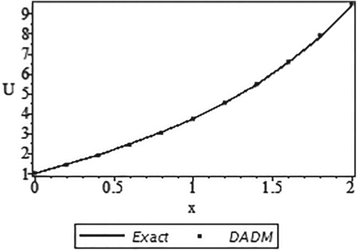
Table 1. The comparison between exact solution $u\left(x\right)$ and the approximate solution using DADM based on the Trapezoidal rule.

x	Exact	DADM	Absolute Error
0	1.00000000	1.00000000	0
0.20	1.42140276	1.42140311	3.51966153e−07
0.40	1.89182470	1.89183726	1.25586920e−05
0.60	2.42211880	2.42222676	1.07957623e−04
0.80	3.02554093	3.02606413	5.23203886e−04
1	3.71828183	3.72014498	1.86315626e−03

Here, the results produced by our method with only few components (m = 5) are in a very good agreement with the exact solution results. Figure 1 clearly shows that all the values of DADM overlapped the values of the exact solutions which give our method an edge over other reported methods of solving system of integro-differential equations.

Moreover, Table 2 and Figure 2 compare the exact solution $v\left(x\right)$ and its approximate solution using DADM based on Trapezoidal rule. Only five components were used from x = 0 to x = 1 at an interval of 0.2 and the respective absolute errors are presented.

Figure 2. Curves of the exact solution $v\left(x\right)$ and the approximate solution using DADM based on the Trapezoidal rule.

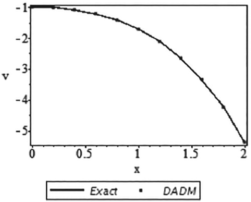
Table 2. The comparison between exact solution $v\left(x\right)$ and the approximate solution using DADM based on the Trapezoidal rule.

x	Exact	DADM	Absolute Error
0	−1.00000000	−1.00000000	0
0.20	−1.02140276	−1.02140264	1.17998654e−07
0.40	−1.09182470	−1.09182052	4.17977601e−06
0.60	−1.22211880	−1.22208370	3.50985477e−05
0.80	−1.42554093	−1.42537777	1.63155502e−04
1	−1.71828183	−1.71773462	5.47210550e−04

In a similar manner, it can be deduced from Table 2 and Figure 2 that the results produced by our method with only a few components (m = 5) are in a very good agreement with the exact solution results. In fact, Figure 2 clearly shows that all the values of DADM overlapped the values of the exact solutions which give our method an edge over other reported methods of solving system of integro-differential equations.

(ii) Simpson's Method

We divide the interval (0, 1) into subinterval of equal lengths $h=.05,n=5$ and denote $x_i=a+ih,0\le i\le 20$, the recursive relation is given by $\left\{\begin{array}{l}{u}_0=2x+1+\frac{1}{2}{x}^2-\frac{1}{60}{x}^5,\\ v_0=-1-\frac{1}{2}{x}^2+\frac{1}{12}{x}^4,\end{array}\right.$ $\left\{\begin{array}{l}{u}_{k+1}=-\frac{1}{2}{L}^{-1}{A}_k\left(x\right)+\frac{.05}{6}{L}^{-1}\left(x\right(B_k\left(t_0\right)+C_k\left(t_0\right))\\ +4\sum _{i=1}^{10}x.\left(B_k\right(t_{2i-1})+C_k(t_{2i-1}\left)\right)+2\sum _{i=1}^{9}x.\left(B_k\right(t_{2i})\\ +C_k\left(t_{2i}\right))+x(B_k\left(t_{20}\right)+C_k\left(t_{20}\right)),k\ge 0,\\ v_{k+1}=-L^{-1}x.u_k\left(x\right)+\frac{.05}{12}{L}^{-1}\left(x\right(B_k\left(t_0\right)-C_k\left(t_0\right))\\ +4\sum _{i=1}^{10}x.\left(B_k\right(t_{2i-1})-C_k(t_{2i-1}\left)\right)+2\sum _{i=1}^{9}x.\left(B_k\right(t_{2i})\\ -C_k\left(t_{2i}\right))+x(B_k\left(t_{20}\right)-C_k\left(t_{20}\right)),k\ge 0,\end{array}\right.$or $\left\{\begin{array}{l}{u}_1=0.16666667x^3+0.04166667x^4+\dots ,\\ v_1=-\frac{1}{6}{x}^3-0.125x^4+\dots ,\\ u_2=-0.025x^5-0.01388889x^6+\dots ,\\ v_2=-0.00555555x^6-0.00039682x^7+\dots ,\\ ⋮\end{array}\right.$

The series solution is then obtained by summing the above iterations as in Equation (14). Table 3 and Figure 3 present the comparison between the exact solution $u\left(x\right)$ and its approximate solution using DADM based on Simpson's rule. Only five components were used from x = 0 to x = 0.5 at an interval of 0.1 and the respective absolute errors are presented.

Figure 3. Curves of the exact solution $u\left(x\right)$ and the approximate solution using DADM based on the Simpson's rule.

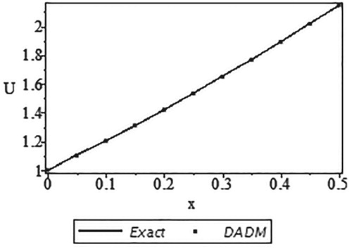
Table 3. The comparison between the exact solution $u\left(x\right)$ and the approximate solution using DADM based on the Simpson's rule.

x	Exact	DADM	Absolute Error
0	1.00000000	1.00000000	0
0.10	1.20517092	1.20517092	1.42545776e−15
0.20	1.42140276	1.42140276	1.86990969e−13
0.30	1.64985881	1.64985881	2.00290725e−12
0.40	1.89182470	1.89182470	3.23009992e−11
0.50	2.14872127	2.14872127	9.09490688e−10

Here, the results produced by our method with only a few components (m = 5) are in a very good agreement with the exact solution results. Besides, Figure 3 clearly shows that all the values of DADM overlapped the values of the exact solutions which give our method an edge over other reported methods of solving system of integro-differential equations.

Moreover, Table 4 and Figure 4 compare the exact solution $v\left(x\right)$ and its approximate solution using DADM based on Simpson's rule. Only five components were used from x = 0 to x = 0.5 at an interval of 0.1 and the respective absolute errors are as well presented.

Figure 4. Curves of the exact solution $v\left(x\right)$ and the approximate solution using DADM based on the Simpson's rule.

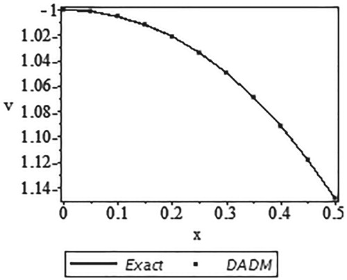
Table 4. The comparison between the exact solution $v\left(x\right)$ and the approximate using DADM based on the Simpson's rule.

x	Exact	DADM	Absolute Error
0	−1.00000000	−1.00000000	0
0.10	−1.00517092	−1.00517092	3.46668166e−16
0.20	−1.02140276	−1.02140276	4.65531657e−14
0.30	−1.04985881	−1.04985881	8.38358300e−13
0.40	−1.09182470	−1.09182470	6.79761258e−12
0.50	−1.14872127	−1.14872127	3.83945477e−11

Similarly, it can be deduced from Table 4 and Figure 4 that the results produced by our method with only few components (m = 5) are in a very good agreement with the exact solution results. In fact, Figure 4 clearly shows that all the values of DADM overlapped the values of the exact solutions which give our method an edge over other reported methods of solving system of integro-differential equations.

Example 2

Consider the system of nonlinear Fredholm integro-differential equation (15) $\left\{\begin{array}{l}{u}^{\mathrm{\prime }\mathrm{\prime }}\left(x\right)=2+\frac{12}{5}x-\underset{0}{\overset{1}{\int }}x\left(u^2+v^2\right)\text{d}t,\\ u\left(0\right)=1,u^{\mathrm{\prime }}\left(0\right)=0,\\ v^{\mathrm{\prime }\mathrm{\prime }}\left(x\right)=-2+\frac{4}{3}x-\underset{0}{\overset{1}{\int }}x\left(u^2-v^2\right)\text{d}t,\\ u\left(0\right)=1,u^{\mathrm{\prime }}\left(0\right)=0,\end{array}\right.$(15) with the exact solution $\left(u\left(x\right),v\left(x\right)\right)=(1+x^2,1-x^2)$

Applying $L^{-1}(.)=\underset{0}{\overset{x}{\int }}\underset{0}{\overset{x}{\int }}(.)\text{d}x\text{d}x$ to both sides of Equation (15), we get, (16) $\left\{\begin{array}{l}u\left(x\right)=1+x^2+\frac{12}{30}{x}^3-L^{-1}\underset{0}{\overset{1}{\int }}x\left(u^2+v^2\right)\text{d}t,\\ v\left(x\right)=1-x^2+\frac{4}{18}{x}^3-L^{-1}\underset{0}{\overset{1}{\int }}x\left(u^2-v^2\right)\text{d}t.\end{array}\right.$(16) (i) Trapezoidal rule

We divide the interval (0, 1) into subinterval of equal lengths $h=.2,n=5$ and denote $x_i=a+ih,0\le i\le 5$, the recursive relation is given by $\left\{\begin{array}{l}{u}_0=1+x^2+\frac{12}{30}{x}^3,\\ v_0=1-x^2+\frac{4}{18}{x}^3,\end{array}\right.$ $\left\{\begin{array}{l}{u}_{k+1}=-.1L^{-1}\left(x\right(A_k\left(t_0\right)+B_k\left(t_0\right))+2\sum _{i=1}^{4}x.(A_k\left(t_i\right)\\ +B_k\left(t_i\right))+x(A_k\left(t_0\right)+B_k\left(t_0\right)),k\ge 0,\\ v_{k+1}=-.1L^{-1}\left(x\right(A_k\left(t_0\right)-B_k\left(t_0\right))+2\sum _{i=1}^{4}x.(A_k\left(t_i\right)\\ -B_k\left(t_i\right))+x(A_k\left(t_0\right)-B_k\left(t_0\right)),k\ge 0,\end{array}\right.$or $\left\{\begin{array}{l}{u}_1=-0.47488288x^3,\\ v_1=-0.28306869x^3,\\ u_2=0.09110678x^3,\\ v_2=0.06979518x^3,\\ ⋮\end{array}\right.$

The series solution is obtained by summation as in Equation (14). We present the comparison of the exact solution u(x) and its approximate solution using DADM based on Trapezoidal rule in Table 5 and Figure 5. Only five components were used from x = 0 to x = 1 at an interval of 0.2 and the respective absolute errors are presented.

Figure 5. Curves of the exact solution $u\left(x\right)$ and the approximate solution using DADM based on the Trapezoidal rule.

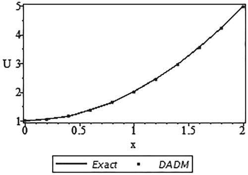
Table 5. The comparison between the exact solution $u\left(x\right)$ and the approximate solution using DADM based on the Trapezoidal rule.

x	Exact	DADM	Absolute Error
0	1.00000000	1.00000000	0
0.20	1.04000000	1.03996370	3.62969667e−05
0.40	1.16000000	1.15970962	2.90375734e−04
0.60	1.36000000	1.35901998	9.80018101e−04
0.80	1.64000000	1.63767699	2.32300587e−03
1	2.00000000	1.99546288	4.53712084e−03

Here, the results produced by our method with only few components (m = 5) are in a very good agreement with the exact solution results. Figure 5 clearly shows that all the values of DADM overlapped the values of the exact solutions which give our method an edge over other reported methods of solving system of integro-differential equations.

Moreover, Table 6 and Figure 6 compare the exact solution v(x) and its approximate solution using DADM based on Trapezoidal rule. Only five components were used from x = 0 to x = 1 at an interval of 0.2 and the respective absolute errors are presented.

Figure 6. Curves of the exact solution $v\left(x\right)$ and the approximate solution using DADM based on the Trapezoidal rule.

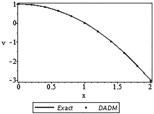
Table 6. The comparison between the exact solution $v\left(x\right)$ and the approximate solution using DADM based on the Trapezoidal rule.

x	Exact	DADM	Absolute Error
0	1.00000000	1.00000000	0
0.20	0.96000000	0.95996436	3.56392238e−05
0.40	0.84000000	0.83971489	2.85113790e−04
0.60	0.64000000	0.63903774	9.62259042e−04
0.80	0.36000000	0.35771909	2.28091032e−03
1	0	−0.00445490	4.45490297e−03

In similar manner, it can be deduced from Table 6 and Figure 6 that the results produced by our method with only a few components (m = 5) are in a very good agreement with the exact solution results. In fact, Figure 6 clearly shows that all the values of DADM overlapped the values of the exact solutions which give our method an edge over other reported methods of solving system of integro-differential equations.

(ii) Simpson's Method

Again, we divide the interval (0, 1) into subinterval of equal lengths $h=.05,n=5$ and denote $x_i=a+ih,0\le i\le 20$, the recursive relation is expressed by $\left\{\begin{array}{c}{u}_0=1+x^2+\frac{12}{30}{x}^3,\\ v_0=1-x^2+\frac{4}{18}{x}^3,\end{array}\right.$ $\left\{\begin{array}{l}{u}_{k+1}=-\frac{.05}{3}{L}^{-1}\left(x\right(A_k\left(t_0\right)+B_k\left(t_0\right))+4\sum _{i=1}^{10}x.(A_k\left(t_{2i-1}\right)\\ +B_k\left(t_{2i-1}\right))+2\sum _{i=1}^{10}x.(A_k\left(t_{2i}\right)+B_k\left(t_{2i}\right))\\ +x\left(A_k\right(t_{20})+B_k(t_{20}\left)\right),k\ge 0,\\ v_{k+1}=-\frac{.05}{3}{L}^{-1}\left(x\right(A_k\left(t_0\right)-B_k\left(t_0\right))+4\sum _{i=1}^{10}x.(A_k\left(t_{2i-1}\right)\\ -B_k\left(t_{2i-1}\right))+2\sum _{i=1}^{10}x.(A_k\left(t_{2i}\right)-B_k\left(t_{2i}\right))\\ +x\left(A_k\right(t_{20})-B_k(t_{20}\left)\right),k\ge 0,\end{array}\right.$or $\left\{\begin{array}{l}{u}_1=-0.46671424x^3,\\ v_1=-0.27423919x^3,\\ u_2=0.08423145x^3,\\ v_2=006319215x^3,\\ ⋮\end{array}\right.$The series solution then follows from Equation (14). We give the comparison of the exact solution $u\left(x\right)$ and its approximate solution using DADM based on Simpson's rule in Table 7 and Figure 7. Only five components were used from x = 0 to x = 0.5 at an interval of 0.1 and the respective absolute errors are presented.

Figure 7. Curves of the exact solution $u\left(x\right)$ and the approximate solution using DADM based on the Simpson's rule.

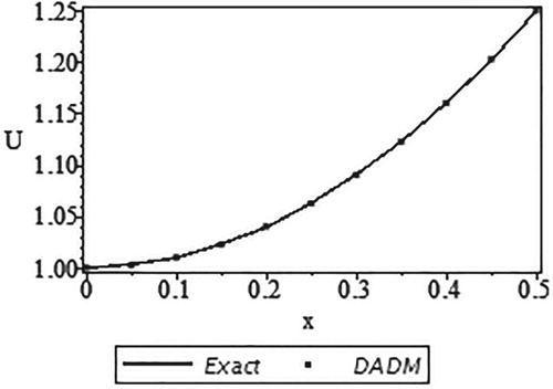
Table 7. The comparison between the exact solution $u\left(x\right)$ and the approximate solution using DADM based on the Simpson's rule.

x	Exact	DADM	Absolute Error
0	1.00000000	1.00000000	0
0.10	1.01000000	1.00999945	5.47032873e−07
0.20	1.04000000	1.03999562	4.37626298e−06
0.30	1.09000000	1.08998523	1.47698876e−05
0.40	1.16000000	1.15996499	3.50101039e−05
0.50	1.25000000	1.24993162	6.83791091e−05

Here, the results produced by our method with only few components (m = 5) are in a very good agreement with the exact solution results. Figure 7 clearly shows that all the values of DADM overlapped the values of the exact solutions which give our method an edge over other reported methods of solving system of integro-differential equations.

Moreover, Table 8 and Figure 8 compare the exact solution $v\left(x\right)$ and its approximate solution using DADM based on Simpson's rule. Only five components were used from x = 0 to x = 0.5 at an interval of 0.1 and the respective absolute errors are presented.

Figure 8. Curves of the exact solution $v\left(x\right)$ and the approximate solution using DADM based on the Simpson's rule.

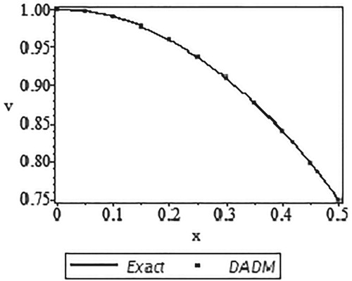
Table 8. The comparison between the exact solution $v\left(x\right)$ and the approximate solution using DADM based on the Simpson's rule.

x	Exact	DADM	Absolute Error
0	1.00000000	1.00000000	0
0.1	0.99000000	0.98999967	3.28891242e−07
0.20	0.96000000	0.95999737	2.63112993e−06
0.30	0.91000000	0.90999112	8.88006352e−06
0.40	0.84000000	0.83997895	2.10490395e−05
0.50	0.75000000	0.74995889	4.11114052e−05

In a similar manner, it can be deduced from Table 8 and Figure 8 that the results produced by our method with only a few components (m = 5) are in a very good agreement with the exact solution results. In fact, Figure 8 clearly shows that all the values of DADM overlapped the values of the exact solutions which give our method an edge over other reported methods of solving system of integro-differential equations.

5. Conclusion

In conclusion, a numerical method for solving system of integro-differential equations is proposed. The method is based on the Discrete Adomian Decomposition Method (DADM) coupled to some numerical integration schemes. The method was further applied to solve the system of nonlinear Volterra and Fredholm integro-differential equations. The proposed method is easy to apply apart being superior to some existing methods in reaching out to approximate solutions. Further, the method is capable of reducing the huge computational steps compared to some classical methods thereby obtaining better accuracy with small number of iterations. Thus, the method can be applied to many integro-differential equations arising in real-life applications.

Disclosure statement

No potential conflict of interest was reported by the authors.

ORCID

H. O. Bakodah http://orcid.org/0000-0003-1403-5936

M. Al-Mazmumy http://orcid.org/0000-0003-3612-004X

S. O. Almuhalbedi http://orcid.org/0000-0001-6126-1982

References

- Delves LM, Mohamed JL. Computational methods for integral equations. Cambridge: Cambridge University Press; 1985.
- Enright WH, Hu M. Continuous Runge-Kutta methods for neutral Volterra integro-differential equations with delay. Appl Numl Math. 1997;24:175–190. doi: 10.1016/S0168-9274(97)00019-6
- Akyuz A, Sezer M. A Chebyshev collocation method for the solution of linear integro-differential equation. Int J Comp Math. 1999;72:491–507. doi: 10.1080/00207169908804871
- Karamete A, Sezer M. A Taylor collocation method for the solution of linear integro-differential equations. Int J Comp Math. 2002;79:987–1000. doi: 10.1080/00207160212116
- Maleknejad K, Mirzaee F, Abbasbandy S. Solving linear integro-differential equations system by using rationalized Haar functions method. Appl Math Computa. 2004;155:317–328. doi: 10.1016/S0096-3003(03)00778-1
- Maleknejad K, Kajani MT. Solving linear integro-differential equation system by Galerkin methods with hybrid functions. Appl Math Computa. 2004;159:603–612. doi: 10.1016/j.amc.2003.10.046
- Wazwaz AM. A first course in integral equations. Singapore: World Scientific Publishing Co. Pte. Ltd; 2015.
- Bakodah HO. Some modifications of Adomian decomposition method applied to nonlinear system of Fredholm integral equations of the second kind. Int J Contemp Math Sci. 2012;7:929–942.
- Bakodah HO. A new modification of the Laplace Adomian decomposition method for system of integral equations. J Am Sci. 2012;8:241–246.
- Bakodah HO. A comparison study between a Chebyshev collocation method and the Adomian decomposition method for solving linear system of Fredholm integral equations of the second kind. J King AbdulAziz Uni Sci. 2012;24:49–59. doi: 10.4197/Sci.24-1.4
- Khan RH, Bakodah HO. Adomian decomposition method and its modification for nonlinear Abel’s integral equation. Int J Math Anal. 2013;7:2349–2358. doi: 10.12988/ijma.2013.37179
- Bakodah HO, Al-Mazmumy M. Almuhalbedi SO. An efficient modification of the Adomian decomposition method for solving integro-differential equations. Math Sci Lett. 2017;6:1–7. doi: 10.18576/msl/060103
- Jafari H, Tayyebi E, Sadeghi S, et al. A new modification of the Adomian decomposition method for nonlinear integral equations. Int J Adv Appl Math Mech. 2014;1(4):33–39.
- Biazar J, Babolian E, Islam R. Solution of a system of Volterra integral equations of the first kind by Adomian method. Appl Math Comput. 2003;139:249–258.
- Wazwaz A. The combined Laplace transform–adomian decomposition method for handling nonlinear Volterra integro–differential equations. Appl Math Comput. 2010;216:1304–1309.
- Ghorbani A, Saberi-Nadjafi J. Exact solutions for nonlinear integral equations by a modified homotopy perturbation method. Comput Math Appl. 2008;56:1032–1039. doi: 10.1016/j.camwa.2008.01.030
- Behiry SH, Abd-Elmonem RA, Gomaa AM. Discrete Adomian decomposition solution of nonlinear Fradholm integral equation. Ain Shams Eng J. 2010;1:97–101. doi: 10.1016/j.asej.2010.09.009
- Bakodah HO, Darwish MA. On discrete Adomian decomposition method with Chebyshev Abscissa for nonlinear integral equations of Hammerstein type. Adv Pure Math. 2012;2:310–313. doi: 10.4236/apm.2012.25042
- Bakodah HO, Darwish MA. Solving Hammerstein type integral equation by new discrete Adomian decomposition methods. Math Prob Eng. 2013;2013:1–5.
- Bakodah HO, Darwish MA. Numerical solutions of quadratic integral equations. Life Sci J. 2014;11:73–77.
- Wazwaz AM. A new algorithm for calculating Adomian polynomials for nonlinear operators. Appl Math Comput. 2000;111:53–69.
- Biazar J, Bablian E, Islam R. An alternative algorithm for computing Adomian polynomials in special cases. Appl Math Comput. 2003;138:523–529.
- Wazwaz AM. A comparison between the Adomian’s decomposition method and Taylor series method in the series solutions. Appl Math Comput. 1999;102:77–86.
- Nuruddeen RI, Muhammad L, Iliyasu R. Two-step modified natural decomposition method for nonlinear Klein-Gordon equations. Nonlinear Stud. 2018;25:743–751.
- Khan U, Ellahi R, Khan R, et al. Extracting new solitary wave solutions of Benny-Luke equation and Phi-4 equation of fractional order by using (G′/G)-expansion method. Opt Quantum Electron. 2017;49:362–373. doi: 10.1007/s11082-017-1191-4
- Demirkus D. Antisymmetric bright solitary SH waves in a nonlinear heterogeneous plate. Z Angew Math Phys. 2018;69:1–17. doi: 10.1007/s00033-018-1010-1
- Nuruddeen RI, Nass AM. Exact solitary wave solution for the fractional and classical GEW-Burgers equations: an application of Kudryashov method. J Taibah Uni Sci. 2018;12:309–314. doi: 10.1080/16583655.2018.1469283
- Bakodah HO, Al-Zaid NA. Computational approaches to initial boundary value problems with Neumann boundary conditions. J Taibah Uni Sci. 2018;18:612–619. doi: 10.1080/16583655.2018.1513688
- Sabi’u J, Jibril A, Gadu AM. New exact solution for the (3 + 1) conformable space-time fractional modified Korteweg–de-Vries equations via Sine-Cosine method. J Taibah Uni Sci. 2019;13(1):91–95. doi: 10.1080/16583655.2018.1537642