Accurate numerical method for Liénard nonlinear differential equations

ABSTRACT

This study introduces a sixth order numerical method for solving Liénard second order nonlinear differential equations. First, the second order Liénard differential equation is transformed into a first order system of equations. Then, the given interval is discretized, and the method is formulated by using Newton's backward difference interpolation formula. The stability and convergence analysis is studied. Three model examples have been presented to demonstrate the reliability and efficiency of the method. The numerical results presented in the tables and graphs show that the present method approximates the exact solution very well.

KEYWORDS:

• Liénard equation
• predictor-corrector method
• consistency

1. Introduction

The real world problems in scientific fields such as solid state physics, plasma physics, fluid mechanics, chemical kinetics and mathematical biology are nonlinear in general when formulated as differential equations [1]. Most of the nonlinear differential equations are complicated to be solved using analytical techniques, but these problems are tackled using approximate analytical or numerical methods. For example, various nonlinear differential equations have been solved using the Taylor matrix method, the closed-form method, Chebyshev polynomial approximations, the variational iteration method, the subdomain finite element method, the differential quadrature method, the homotopy perturbation method, the quitic B-spline differential quadrature method, the power series method, the Pade series method, the Legendre polynomial function approximation [2], predictor–corrector method [3], etc.

The Liénard equation is a nonlinear second order differential equation proposed by Liénard [4] and is presented as: (1) $u^{\mathrm{\prime }\mathrm{\prime }}\left(x\right)+p\left(u\right)u^{\mathrm{\prime }}\left(x\right)+q\left(u\right)=g\left(x\right)$(1) subject to the initial conditions $u\left(x_0\right)=\alpha ,u^{\mathrm{\prime }}\left(x_0\right)=\beta$. Equation (1) is not only regarded as a generalization of the damped pendulum equation or a damped spring-mass system (where $p\left(u\right)u^{\mathrm{\prime }}\left(x\right)$ is the damping force, $q\left(u\right)$ is the restoring force, and $g\left(x\right)$ is the external force), but also used as nonlinear models in many physically significant fields when taking different choices for $p\left(u\right),q\left(u\right)$ and $g\left(x\right)$. For example, the choices $p\left(u\right)=\epsilon (u^2-1),q\left(u\right)=u$ and $g\left(x\right)=0$ lead Equation (1) to the Van der Pol equation served as a nonlinear model of electronic oscillation [5,6]. Moreover, in the development of radio and vacuum tube technology, Liénard equations were remarkably investigated as they can be utilized to describe the oscillating circuits [7]. The Liénard-type equations can also be used to model fluid mechanical phenomena [8].

In recent years, many researchers have tried to develop different numerical methods for solving Liénard differential equations. For examples, Equation (1) was studied by many authors in [9–17]. However still, the accuracy of their solution needs improvement. Thus, this study introduces a sixth order predictor–corrector method which is stable, convergent and more accurate for solving Liénard second order ordinary differential equations.

2. Formulation of the method

Let $v\left(x\right)=u^{\mathrm{\prime }}\left(x\right)$, then Equation (1) is changed into a first order system of equations: (2) $\left\{\begin{array}{l}{u}^{\mathrm{\prime }}\left(x\right)=v\left(x\right)=f^{\left(1\right)}(x,u,v),u\left(x_0\right)=\alpha \\ \begin{array}{c}{v}^{\mathrm{\prime }}\left(x\right)=g\left(x\right)-p\left(u\right)v\left(x\right)\\ -q\left(u\right)=f^{\left(2\right)}(x,u,v)\end{array},v\left(x_0\right)=\beta \end{array}\right.$(2) To describe the methods, let's denote $u^{\left(1\right)}=u$ and $u^{\left(2\right)}=v$, then Equation (2) can be written as: (3) $\frac{d{u}^{\left(j\right)}}{dx}=f^{\left(j\right)}\left(x,u^{\left(1\right)},u^{\left(2\right)}\right),\text{for}j=1,2$(3) subject to $u_0^{\left(1\right)}=\alpha ,u_0^{\left(2\right)}=\beta$.

Now, divide the interval $[x_0,L]$ into N equal subintervals of mesh length h and integrating Equation (3) on the interval $\left[x_i,x_{i+1}\right]$, we obtain: (4) $\begin{array}{rl}{u}^{\left(j\right)}\left(x_{i+1}\right)& =u^{\left(j\right)}\left(x_i\right)+{\int }_{x_i}^{x_{i+1}}{f}^{\left(j\right)}(x,u^{\left(1\right)},u^{\left(2\right)})\text{d}x,\\ & \text{for}j=1,2\end{array}$(4) To formulate the methods, we approximate $f^{\left(j\right)}(x,u^{\left(1\right)},u^{\left(2\right)}),\text{for}j=1,2$ by a suitable interpolation polynomials.

Case 1: Take k data values $\left(x_i,f_i^{\left(j\right)}\right),\left(x_{i-1},f_{i-1}^{\left(j\right)}\right),\dots ,({x_{i-}}_{k+1},f_{i-k+1}^{\left(j\right)})$, for $j=1,2$. For this data, we fit Newton's backward difference interpolating polynomial of degree $k-1$ and obtain: (5) $f^{\left(j\right)}\left(x_i+sh\right)=\sum _{m=0}^{k-1}{(-1)}^m\left(\begin{array}{c}-s\\ m\end{array}\right){\mathrm{\nabla }}^m{f}_i^{\left(j\right)}+t_k^{\left(j\right)}$(5) where $s=\left(\right(x-x_i\left)/h\right)$ and (6) $t_k^{\left(j\right)}=\frac{s\left(s+1\right)\left(s+2\right)\dots (s+k-1)}{k!}{h}^k{f}^{\left(j\right)}\left(\xi \right)$(6) is the error term, when $\xi$ lies in some interval containing the points $x_i,x_{i-1,\dots ,}{x}_{i-k+1}$ and x.

Using Equations (5) and (6) in Equation (4), we get: (7) $u_{i+1}^{\left(j\right)}=u_i^{\left(j\right)}+h{\int }_0^1\left(\sum _{m=0}^{k-1}{(-1)}^m\left(\begin{array}{c}-s\\ m\end{array}\right){\mathrm{\nabla }}^m{f}_i^{\left(j\right)}+t_k^{\left(j\right)}\right)\text{d}s$(7) Integrating term by term, Equation (7) with respect to s, choosing the value $k=6$ and simplifying, we obtain: (8) $\begin{array}{rl}{u}_{i+1}^{\left(j\right)}& =u_i^{\left(j\right)}+\frac{h}{1440}\left\{4277f_i^{\left(j\right)}-7923f_{i-1}^{\left(j\right)}+9982f_{i-2}^{\left(j\right)}\right.\\ & -\left.7298f_{i-3}^{\left(j\right)}+2877f_{i-4}^{\left(j\right)}-475f_{i-5}^{\left(j\right)}\right\}+{\tau }_6^{\left(j\right)}\end{array}$(8) where (9) ${\tau }_6^{\left(j\right)}=\frac{19087}{60480}{h}^7(u^{\left(j\right)}{)}^{\left(6\right)}\left(\xi \right),\text{for}j=1,2$(9) is the local truncation error. Hence, Equation (8) is called predictor method.

Case 2: Consider the $k+1$ data values $\left(x_{i+1},f_{i+1}^{\left(j\right)}\right),\left(x_i,f_i^{\left(j\right)}\right),\dots ,({x_{i-}}_{k+1},f_{i-k+1}^{\left(j\right)})$, for $j=1,2$, which include the current data points. For this data, we fit Newton's backward difference interpolating polynomial of degree k and obtain: (10) $f^{\left(j\right)}\left(x_i+sh\right)=\sum _{m=0}^k{(-1)}^m\left(\begin{array}{c}1-s\\ m\end{array}\right){\mathrm{\nabla }}^m{f}_{i+1}^{\left(j\right)}+T_k^{\left(j\right)}$(10) where $s=\left(\right(x-x_i\left)/h\right)$, $x-x_{i+1}=(x-x_i)-(x_{i+1}-x_i)=sh-h=h(s-1)$ and (11) $T_k=\frac{\left(s-1\right)s\left(s+1\right)\left(s+2\right)\dots \left(s+k-1\right)}{\left(k+1\right)!}{h}^{k+1}{f}^{\left(j\right)}\left(\xi \right)$(11) is the error term, when $\xi$ lies in some interval containing the points $x_{i+1},x_i,x_{i-1},\dots ,x_{i-k+1}$ and x.

Using Equations (10) and (11) in Equation (4), we get: (12) $\begin{array}{rl}{u}_{i+1}^{\left(j\right)}& =u_i^{\left(j\right)}+h{\int }_0^1\left(\sum _{m=0}^k{(-1)}^m\left(\begin{array}{c}1-s\\ m\end{array}\right)\right.\\ & \times \left.{\mathrm{\nabla }}^m{f}_{i+1}^{\left(j\right)}+T_k^{\left(j\right)}\right)\text{d}s\end{array}$(12) Integrating term by term, Equation (12) with respect to s, choosing $k=5$ and simplifying, we get: (13) $\begin{array}{rl}{u}_{i+1}^{\left(j\right)}& =u_i^{\left(j\right)}+\frac{h}{1440}\{475f_{i+1}^{\left(j\right)}+1427f_i^{\left(j\right)}-798f_{i-1}^{\left(j\right)}\\ & +482f_{i-2}^{\left(j\right)}-173f_{i-3}^{\left(j\right)}+27f_{i-4}^{\left(j\right)}\}+{\tau }_5^{\left(j\right)}\end{array}$(13) where $f_{i+1}^{\left(j\right)}=f^{\left(j\right)}\left(x_{i+1},u_{i+1}^{\left(1\right)},u_{i+1}^{\left(2\right)}\right)$ and $u_{i+1}^{\left(1\right)},u_{i+1}^{\left(2\right)}$ are values obtained from Equation (8) and (14) ${\tau }_5^{\left(j\right)}=-\frac{863}{60480}{h}^7(u^{\left(j\right)}{)}^{\left(6\right)}\left(\xi \right),\text{for}j=1,2$(14) is the local truncation error of a corrector method.

Thus, Liénard second order nonlinear differential equation in Equation (1) can be easily solved by the systems in Equations (8) and (13) using MATLAB software.

Remark 2.1:

For using these methods, we require the starting values $u_0^{\left(j\right)},u_1^{\left(j\right)},u_2^{\left(j\right)},u_3^{\left(j\right)},u_4^{\left(j\right)}$, for $j=1,2$. So in this study, we used the classical Runge–Kutta method for the first five nodal points.

3. Stability and convergence analysis

Definition 3.1:

Let ${\lambda }_1,{\lambda }_2,\dots ,{\lambda }_k$ and ${\gamma }_1,{\gamma }_2,\dots ,{\gamma }_k$ are respectively the (not necessarily distinct) roots of the characteristic equations given by: $\begin{array}{rl}{p}_1\left(\lambda \right)& ={\lambda }^k-a_{k-1}^{\left(1\right)}{\lambda }^{k-1}-\cdots -a_1^{\left(1\right)}\lambda -a_0^{\left(1\right)}=0,\\ & \text{for}j=1,2\end{array}$ $\begin{array}{rl}{p}_2\left(\gamma \right)& ={\gamma }^k-a_{k-1}^{\left(2\right)}{\gamma }^{k-1}-\cdots -a_1^{\left(2\right)}\gamma -a_0^{\left(2\right)}=0,\\ & \text{for}j=1,2\end{array}$associated with the system of the multistep difference method of Equations (8) and (13) given as: $\begin{array}{rl}{u}_{i+1}^{\left(j\right)}& =a_{k-1}^{\left(j\right)}{u}_i^{\left(j\right)}+a_{k-2}^{\left(j\right)}{u}_{i-1}^{\left(j\right)}+\dots +a_0^{\left(j\right)}{u}_{i+1-k}^{\left(j\right)}\\ & +hF\left(x_i,h,u_{i+1}^{\left(j\right)},u_i^{\left(j\right)},\dots ,u_{i+1-k}^{\left(j\right)}\right),\end{array}$where $a_0^{\left(j\right)},a_1^{\left(j\right)},\dots ,a_{k-1}^{\left(j\right)}$ are constants, for each $i=k-1,k,\dots ,N-1$ and $j=1,2$.

If $|{\lambda }_i|\le 1,$ and $|{\gamma }_i|\le 1$ for $i=1,2,\dots ,k,$ and all roots with absolute value 1 are simple roots, then the system of the difference method is said to satisfy the root condition.

Definition 3.2:

Method that satisfy the root condition and have $\lambda =1$ as the only root of the characteristic equation with magnitude one is called strongly stable [18].

Theorem 3.1:

The scheme in Equation (8) is strongly stable.

Proof:

The scheme in Equation (8) can be expressed as: $u_{i+1}^{\left(j\right)}=u_i^{\left(j\right)}+hF\left(x_i,h,u_i^{\left(j\right)},u_{i-1}^{\left(j\right)},u_{i-2}^{\left(j\right)}{u}_{i-3}^{\left(j\right)},u_{i-4}^{\left(j\right)},u_{i-5}^{\left(j\right)}\right),$where $\begin{array}{rlr}& F\left(x_i,h,u_i^{\left(j\right)},u_{i-1}^{\left(j\right)},u_{i-2}^{\left(j\right)}{u}_{i-3}^{\left(j\right)},u_{i-4}^{\left(j\right)},u_{i-5}^{\left(j\right)}\right)& \\ & =\frac{1}{1440}\left\{4277f^{\left(j\right)}\right(x_i,u_i^{\left(1\right)},u_i^{\left(2\right)})\\ & -7923f^{\left(j\right)}(x_{i-1},u_{i-1}^{\left(1\right)},u_{i-1}^{\left(2\right)})\\ & +9982f^{\left(j\right)}(x_{i-2},u_{i-2}^{\left(1\right)},u_{i-2}^{\left(2\right)})\\ & -7298f^{\left(j\right)}(x_{i-3},u_{i-3}^{\left(1\right)},u_{i-3}^{\left(2\right)})\\ & +2877f^{\left(j\right)}(x_{i-4},u_{i-4}^{\left(1\right)},u_{i-4}^{\left(2\right)})\\ & -475f^{\left(j\right)}(x_{i-5},u_{i-5}^{\left(1\right)},u_{i-5}^{\left(2\right)})\}\end{array}$In this case, $k=6$ so by Definition 3.1, we have:

$a_0^{\left(j\right)}=a_1^{\left(j\right)}=a_2^{\left(j\right)}=a_3^{\left(j\right)}=a_4^{\left(j\right)}=0,\text{and}{a}_5^{\left(j\right)}=1$, for $j=1,2$.

The characteristic equations for the method becomes: $p_1\left(\lambda \right)={\lambda }^6-{\lambda }^5={\lambda }^5\left(\lambda -1\right)=0,\text{for}j=1,$ $p_2\left(\gamma \right)={\gamma }^6-{\gamma }^5={\gamma }^5\left(\gamma -1\right)=0,\text{for}j=2.$which implies ${\lambda }_1={\gamma }_1=1\text{and}{\lambda }_i={\gamma }_i=0$ for $i=2,3,\dots ,6$ are the roots of the polynomials.

Therefore, the predictor method in Equation (8) satisfies the root condition and is strongly stable by Definition 3.2.

Theorem 3.2:

The scheme in Equation (13) is also strongly stable.

Proof:

The scheme in Equation (13) can be expressed as: $u_{i+1}^{\left(j\right)}=u_i^{\left(j\right)}+hF\left(x_i,h,u_{i+1}^{\left(j\right)},u_i^{\left(j\right)},u_{i-1}^{\left(j\right)},u_{i-2}^{\left(j\right)}{u}_{i-3}^{\left(j\right)},u_{i-4}^{\left(j\right)}\right)$where $\begin{array}{rl}& F\left(x_i,h,u_{i+1}^{\left(j\right)},u_i^{\left(j\right)},u_{i-1}^{\left(j\right)},u_{i-2}^{\left(j\right)}{u}_{i-3}^{\left(j\right)},u_{i-4}^{\left(j\right)}\right)\\ & =\frac{h}{1440}\left\{475f^{\left(j\right)}(x_{i+1},u_{i+1}^{\left(1\right)},u_{i+1}^{\left(2\right)})\right.\\ & +1427f^{\left(j\right)}(x_i,u_i^{\left(1\right)},u_i^{\left(2\right)})\\ & -798f^{\left(j\right)}(x_{i-1},u_{i-1}^{\left(1\right)},u_{i-1}^{\left(2\right)})+482f^{\left(j\right)}(x_{i-2},u_{i-2}^{\left(1\right)},u_{i-2}^{\left(2\right)})\\ & -\left.173f^{\left(j\right)}(x_{i-3},u_{i-3}^{\left(1\right)},u_{i-3}^{\left(2\right)})+27f^{\left(j\right)}(x_{i-4},u_{i-4}^{\left(1\right)},u_{i-4}^{\left(2\right)})\right\}\end{array}$Following the similar procedure as we have done in Theorem 3.1, here, $k=5$ which implies $a_0^{\left(j\right)}=a_1^{\left(j\right)}=a_2^{\left(j\right)}=a_3^{\left(j\right)}=0$ and $a_4^{\left(j\right)}=1$, for $j=1,2$.

The characteristic equations for the method become: $p_1\left(\lambda \right)={\lambda }^5-{\lambda }^4={\lambda }^4\left(\lambda -1\right)=0,\text{for}j=1,$ $p_2\left(\gamma \right)={\gamma }^5-{\gamma }^4={\gamma }^4\left(\gamma -1\right)=0,\text{for}j=2.$Thus, the polynomials have roots ${\lambda }_1={\gamma }_1=1\text{and}{\lambda }_i={\gamma }_i=0$ for $i=2,3,4,5$.

Therefore, the corrector method in Equation (13) satisfies the root condition and is strongly stable by Definition 3.2.

Definition 3.3

Consistency:

The method is consistent if the local truncation error ${\tau }_k\left(h\right)\to 0\text{as}h\to 0$.

Lemma 3.1:

The schemes in Equations (8) and (13) are both sixth-order convergence.

Proof:

From Equations (9) and (14), we have: $\begin{array}{rl}{\tau }_5^{\left(j\right)}& =-\frac{863}{60480}{h}^7(u^{\left(j\right)}{)}^{\left(6\right)}\left(\xi \right)\text{and}\\ {\tau }_6^{\left(j\right)}& =\frac{19087}{60480}{h}^7(u^{\left(j\right)}{)}^{\left(6\right)}\left(\xi \right)\end{array}$Thus, ${\tau }_k^{\left(j\right)}\left(h\right)\to 0\text{as}h\to 0\text{for}k=5,6$ and $j=1,2$

Therefore, the methods in Equations (8) and (13) are consistent and hence they are sixth-order convergence.

4. Numerical examples and Results

Three model examples of Liénard second order nonlinear differential equations with initial conditions have been considered to validate the applicability of the method. For each number of nodal points $N$, the pointwise absolute errors were approximated by the formula $||E||=|u\left(x_i\right)-u_i|$, for $i=0,1,2,\dots ,N$, where $u\left(x_i\right)$ and $u_i$ are exact and computed an approximate solution of the given problems respectively, at the nodal point $x_i$. Numerical examples are presented to illustrate the reliability and efficiency of the method. Comparison of numerical results is made with a Magnus series expansion method [15] which is based on Lie groups and Lie algebras on some specific nonlinear differential equations, a differential transform method [16] based on the Taylor series expansion which constructs an analytical solution in the form of a polynomial and a hybrid heuristic computation [17] based technique as an alternative to the existing deterministic standard numerical methods, including variational iteration method and differential transform method for solving the Liénard differential equations numerically.

Example 4.1:

Consider the following Liénard Equation: $\begin{array}{rl}& u^{\mathrm{\prime }\mathrm{\prime }}\left(x\right)+u\left(x\right)u^{\mathrm{\prime }}\left(x\right)+u\left(x\right)+u^2\left(x\right)\\ & ={\cos }^2\left(x\right)-\sin \left(x\right)\cos \left(x\right)\end{array}$with the initial conditions $u\left(0\right)=1,u^{\mathrm{\prime }}\left(0\right)=0$

The exact solution of the given problem is given by $u\left(x\right)=\cos \left(x\right)$. Numerical results are presented in Tables 1 and 2 and Figures 1 and 2.

Figure 1. Numerical solution versus exact solution for Example 4.1 when $h=0.05$.

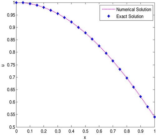
Figure 2. Pointwise absolute errors for Example 4.1 with different values of $h$.

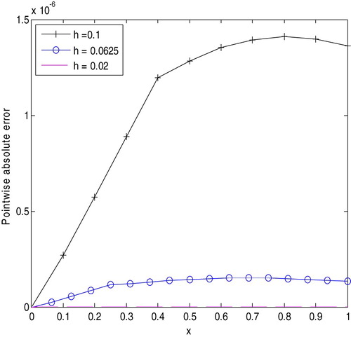
Table 1. The pointwise absolute errors for Example 4.1 with $x\in \left[0,0.5\right]$.

		Present method
$x$	Magnus series [15] h = 0.001	$h=0.1$	$h=0.1$ Refinement	$h=0.01$	$h=0.001$
0		0	0	0	0
0.1	1.4409e−04	2.6794e−07	2.6794e−07	1.2975e−11	4.4409e−16
0.2	1.15476e−03	5.7177e−07	5.7177e−07	1.6940e−11	4.4409e−16
0.3	3.90185e−03	8.8764e−07	8.8764e−07	2.1276e−11	1.3323e−15
0.4	9.2132e−03	1.1954e−06	1.1954e−06	2.4793e−11	1.3323e−15
0.5	1.78199e−02	1.2849e−06	1.2747e−06	2.6595e−11	1.6653e−15

Table 2. The maximum absolute errors for different values of h and $x\in [0,1]$.

$h=1/50$	$h=1/\text{1}00$	$h=1/200$	$h=1/300$	$h=1/400$	$h=1/500$
6.6333e−10	2.6704e−11	1.1988e−12	2.0595e−13	7.2942e−14	2.9088e−14
Refinement
6.7708e−10	2.8566e−11	1.3498e−12	2.3725e−13	6.9500e−14	2.8089e−14

Table 1 exhibits the pointwise absolute errors for different values of mesh size $h$, and it can be seen that the present method improves the findings of Sure et al. [15]. In Table 2, the maximum absolute errors of the present method and its refinement are presented for different values of $h$. From Tables 1 and 2, one can observe that as the mesh size $h$ decreases the absolute errors also decrease.

Example 4.2:

Consider the following Liénard Equation: $u^{\mathrm{\prime }\mathrm{\prime }}\left(x\right)-u\left(x\right)+4u^3\left(x\right)-3u^5\left(x\right)=0$with the initial conditions, $u\left(0\right)=1/sqrt\left(2\right),u^{\mathrm{\prime }}\left(0\right)=sqrt\left(2\right)/4$The exact solution of the given problem is given by $u\left(x\right)=sqrt\left((1+\tanh (x\left)\right)/2\right)$. Numerical results are presented in Tables 3 and 4 and Figures 3 and 4.

Figure 3. Numerical solution versus exact solution for Example 4.2 when $h=0.05$.

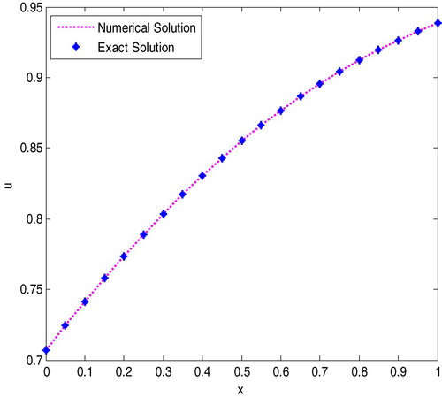
Figure 4. Pointwise absolute errors for Example 4.2 with different values of $h$.

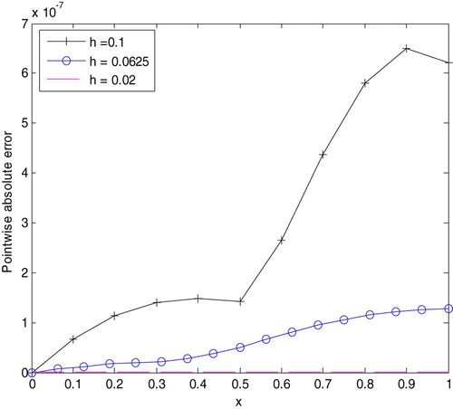
Table 3. The pointwise absolute errors for Example 4.2 with $x\in \left[0,1\right]$ and different values of h.

	Differential transform [16]	Hybrid heuristic computation [17]		Present method
$x$	$h=0.1$	IPA	ASA	$h=0.1$	$h=0.1$ Refinement	$h=0.01$	$h=0.002$
0.1	2.2683e−06	6.24e−06	7.30e−06	6.7141e−08	6.7141e−08	3.1564e−12	1.8874e−15
0.2	2.5222e−06	5.60e−06	7.55e−06	1.1401e−07	1.1401e−07	4.0805e−12	2.9976e−15
0.3	1.4404e−05	5.15e−06	7.75e−06	1.4010e−07	1.4010e−07	5.5097e−12	4.5519e−15
0.4	6.1806e−05	5.08e−06	7.88e−06	1.4855e−07	1.4855e−07	7.2031e−12	6.1062e−15
0.5	2.2099e−04	5.00e−06	7.95e−06	1.4131e−07	1.3523e−07	8.8091e−12	6.9944e−15
0.6	6.5187e−04	4.60e−06	8.06e−06	2.6414e−07	9.8888e−08	9.9460e−12	7.6605e−15
0.7	1.6408e−03	3.96e−06	8.32e−06	4.3610e−07	5.4195e−08	1.0276e−11	7.1054e−15
0.8	3.6469e−03	3.39e−06	8.73e−06	5.8126e−07	1.3746e−08	9.5440e−12	5.1070e−15
0.9	7.3493e−03	3.15e−06	9.18e−06	6.4934e−07	1.4832e−08	7.5914e−12	1.3323e−15
1.0	1.3692e−02	3.18e−06	9.65e−06	6.2114e−07	2.9187e−08	4.3318e−12	5.2180e−15

Table 4. The maximum absolute errors for Example 4.2 for different values of h and $x\in [0,1]$.

$h=1/50$	$h=1/\text{1}00$	$h=1/200$	$h=1/300$	$h=1/400$	$h=1/500$
3.5866e−10	1.0288e−11	3.9369e−13	6.5170e−14	1.8652e−14	7.6605e−15
Refinement
1.5083e−10	7.0087e−12	3.4439e−13	6.1284e−14	1.8208e−14	7.5495e−15

Table 3 exposes the pointwise absolute errors for different values of $h$, and it can be seen that the present method improves the findings of Mashallah et al. [16] and Suheel et al. [17]. Table 4 shows the maximum absolute errors of the present method and its refinement for different values of $h$. In Tables 3 and 4, it can be seen that as the mesh size $h$ decreases the absolute errors also decrease.

Example 4.3:

Consider the following Liénard Equation: $u^{\mathrm{\prime }\mathrm{\prime }}\left(x\right)-u\left(x\right)+4u^3\left(x\right)+3u^5\left(x\right)=0$with the initial conditions, $u\left(0\right)=\frac{1}{\sqrt{1+\sqrt{2}}},u^{\mathrm{\prime }}\left(0\right)=0$

The exact solution of the given problem is given by $u\left(x\right)=\sqrt{\left(\sec h^2\right(x\left)\right)/(2\sqrt{2}+(1-\sqrt{2}\left)\sec h^2\right(x\left)\right)}$.

Numerical results are presented in Tables 5 and 6 and Figure 5.

Figure 5. Numerical solution versus exact solution for Example 4.3 when $h=0.05$.

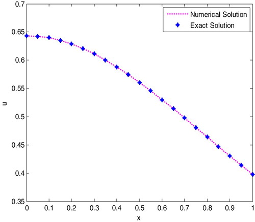
Table 5. The pointwise absolute errors for Example 4.3 with $x\in \left[0,1\right]$ and different values of h.

	Differential transform [16]	Hybrid heuristic computation [17]		Present method
$x$	$h=0.1$	IPA	ASA	$h=0.1$	$h=0.1$ Refinement	$h=0.01$	$h=0.002$
0.1	4.0668e−06	4.33e−05	1.64e−05	2.5685e−08	2.5685e−08	8.5355e−12	8.5487e−15
0.2	3.7000e−06	5.31e−05	2.22e−05	5.1433e−07	5.1433e−07	2.3057e−11	3.2085e−14
0.3	7.1793e−06	5.84e−05	2.55e−05	1.3397e−06	1.3397e−06	4.2467e−11	6.3172e−14
0.4	4.5002e−05	6.37e−05	2.21e−05	2.3254e−06	2.3254e−06	6.3473e−11	9.6034e−14
0.5	2.4676e−04	6.49e−05	1.54e−05	3.3161e−06	3.2340e−06	8.2096e−11	1.2235e−13
0.6	9.9922e−04	6.01e−05	1.11e−05	5.0076e−06	3.8973e−06	9.4586e−11	1.3622e−13
0.7	3.2168e−03	5.27e−05	1.09e−05	7.9779e−06	4.2577e−06	9.8288e−11	1.3467e−13
0.8	8.7371e−03	4.67e−05	1.13e−05	1.2097e−05	4.3703e−06	9.2047e−11	1.1663e−13
0.9	2.0841e−02	4.28e−05	7.47e−06	1.6871e−05	4.3323e−06	7.6092e−11	8.2989e−14
1.0	4.4891e−02	3.83e−05	9.00e−07	2.1802e−05	4.2279e−06	5.1619e−11	3.5860e−14

Table 6. The maximum absolute errors for different values of h and $x\in [0,1]$.

$h=1/50$	$h=1/\text{1}00$	$h=1/200$	$h=1/300$	$h=1/400$	$h=1/500$
2.4198e−09	1.1685e−10	6.4769e−12	1.2325e−12	3.8236e−13	1.5532e−13
Refinement
2.0705e−09	9.8358e−11	5.6958e−12	1.0956e−12	3.3984e−13	1.3756e−13

Table 5 exhibits the pointwise absolute errors for different values of $h$, and it can be seen that the present method improves the findings of Mashallah et al. [16] and Suheel et al. [17]. From Tables 5 and 6, one can observe that as the mesh size $h$ decreases the absolute errors also decrease.

5. Conclusion

This study considered a sixth order predictor–corrector method for solving Liénard second order nonlinear differential equations. The stability and convergence of the method have been investigated. To further collaborate the applicability of the proposed method, tables of absolute errors and graphs have been plotted. Tables 1, 3 and 5 show that the pointwise absolute errors obtained by the present method have been compared with pointwise absolute errors obtained by different authors. From Tables 1–6, one can observe that all the absolute errors decrease rapidly as h decreases, which in turn show the convergence of the computed solution. Figures 1, 3 and 5 indicate that the present method approximates the exact solution very well. Figures 2 and 4 show that as h decreases, the absolute error goes to zero which shows that small step size provides a better approximation.

Concisely, the present method is computationally stable, efficient, convergent and simple to use. Furthermore, it gives more accurate solution than some earlier existing numerical methods, including the more recent method in [15–17].

Disclosure statement

No potential conflict of interest was reported by the authors.

ORCID

Gashu Gadisa Kiltu http://orcid.org/0000-0003-3541-2630

Gemechis File Duressa http://orcid.org/0000-0003-1889-4690

References

- Prajapati RN, Mohan R, Kumar P. Numerical solution of generalized Abel’s integral equation by variational iteration method. Am J Comput Math. 2012;2:312–315. doi: 10.4236/ajcm.2012.24042
- Yüzbas S. A numerical scheme for solutions of a class of nonlinear differential equations. J Taibah Univ Sci. 2017;11:1165–1181. doi: 10.1016/j.jtusci.2017.03.001
- Roba G, Gadisa G, Hailu K. Fifth order predictor-corrector method for quadratic Riccati differential equations. Int J Eng Appl Sci. 2017;9(4):51–64.
- Liénard A. Etude des oscillations entretenues. Rev Gen Electr. 1928;23:901–912 and 946–954.
- Guckenheimer J. Dynamics of the van der Pol equation. IEEE Trans Circ Syst. 1980;27:983–989. doi: 10.1109/TCS.1980.1084738
- Zhang ZF, Ding T, Huang HW, et al. Qualitative theory of differential equations. Peking: Science Press; 1985.
- Kumar D, Agarwal PR, Singh J. A modified numerical scheme and convergence analysis for a fractional model of Liénard’s equation. J Comput Appl Math. 2017. doi: 10.1016/j.cam.2017.03.011
- Harko T, Lobo SNF, Mak MK. A class of exact solutions of the Liénard type ordinary non-linear differential equation. J Eng Math. 2014;89(1):193–205. doi: 10.1007/s10665-014-9696-3
- Feng Z. On explicit exact solutions for the Liénard equation and its applications. Phys Lett A. 2002;293:50–56. doi: 10.1016/S0375-9601(01)00823-4
- Kong D. Explicit exact solutions for the Liénard equation and its applications. Phys Lett A. 1995;196:301–306. doi: 10.1016/0375-9601(94)00866-N
- Matinfar M, Hosseinzadeh H, Ghanbari M. A numerical implementation of the variational iteration method for the Liénard equation. World J Model Simul. 2008;4:205–210.
- Matinfar M, Mahdavi M, Raeisy Z. Exact and numerical solution of Liénard’s equation by the variational homotopy perturbation method. J Inf Comput Sci. 2011;6(1):73–80.
- Sun J, Wang W, Wu L. On explicit exact solutions for the Liénard equation and its applications. Phys Lett A. 2003;318:93–101. doi: 10.1016/j.physleta.2003.07.027
- Kaya D, El-Sayed SM. A numerical implementation of the decomposition method for the Liénard equation. Appl Math Comput. 2005;171:1095–1103.
- Sure K, Aytekin E, Mehmet TA. A numerical approximation to some specific nonlinear differential equations using Magnus series expansion method. NTMSCI. 2016;4(1):125–129. doi: 10.20852/ntmsci.2016115660
- Mashallah M, Saber RB, Maryam G. Solving the Liénard equation by differential transform method. World J Model Simul. 2012;8(2):142–146.
- Suheel AM, Ijaz MQ, Muhammad A, et al. Numerical solution of Liénard equation using Hybrid Heuristic computation. World Appl Sci J. 2013;28(5):636–643.
- Eberly D. Stability analysis for systems of differential equations. Mountain View: Geometric Tools, LLC; 2008.