On the difference equation z_m+1 = f(z_m, z_m-1, …, z_m–k)

Abstract

In the present work, we investigate the stability, periodicity and oscillation of the solution for a new general class of difference equations. Actually, this is the most general form of linear difference equations. Hence, the results in this article apply to several other equations that are special cases of the proposed equation. We also use an efficient method to study periodic solution of period two, with no restriction of the coefficients of difference equations, i.e. they are arbitrary real numbers. Finally, we give three applications of these equations to support our analysis.

Keywords:

• Difference equation
• equilibrium points
• local stability
• prime period two solution
• oscillation

AMS subject classifications:

• 39A10
• 39A23
• 39A30

1. Introduction

During the past four decades the study of difference equations was the main goal for many researchers. Many robust methods for studying asymptotic behaviour of the difference equations have been proposed and developed. Many researchers were interested of studying the qualitative behaviour of various types of difference equations. This highly interesting due to the fact that these equations describe daily life phenomena in physics, quanta in radiation, biology, probability theory, electrical network, etc.

Oscillation theory of difference equations attracted a considerable attention in the recent years. It was shown that the results of this theory were in many aspects similar to those of the oscillation theory of differential equations, even if one has in many cases to use different methods or substantially modify methods continuous oscillation theory.

The oscillation and global asymptotic behaviour of the solutions were two such qualitative properties that are so important for applications in many areas such as biology, control theory, game theory, engineering, economy and neural networks. It is so difficult to use numerical techniques to study the oscillation or the asymptotic behaviour of all solutions of a given equation due to the global nature of these properties. Thus, these properties have received the attention of several mathematicians, physicists and engineers.

The purpose of this paper is to investigate the asymptotic behaviour of the solutions of a general class of difference equation (1) $z_{m+1}=f\left(z_m,z_{m-1},\dots ,z_{m-k}\right),$(1) where k is positive integer and the function $f:(0,\mathrm{\infty }{)}^{k+1}\to (0,\mathrm{\infty })$ is continuous real function and homogenous with degree zero. The construction of this new class of difference equations was complex and involves several cases. There were so many work about the asymptotic behaviour of solutions for the nonlinear difference equations [1–28].

The outputs of this article made three major contributions to the study of linear difference equations. First, we formulated a general class of difference equations as a means of establishing general theorems for the asymptotic behaviour of its solutions and the solutions of equations that are special cases of the studied equation. Second, we used an efficient method introduced in [13] and its modification in [20,21] in compact and accurate way, namely in Theorems 3.1 and 3.2. This method is valid to apply for many difference equations, which are failed to solve by the classical method. Third, we gave some new applications of these homogenous difference equations.

This work is organized as follows: In Section 2, we presented the stability behaviour of the solution for Equation (1(1) $z_{m+1}=f\left(z_m,z_{m-1},\dots ,z_{m-k}\right),$(1) ). In Section 3 we used a motivated method to study the periodic behaviour of the solution for Equation (1(1) $z_{m+1}=f\left(z_m,z_{m-1},\dots ,z_{m-k}\right),$(1) ). This technique had a very characteristic feature, i.e. the coefficients of difference equations are arbitrary real numbers. In Section 4 we study the oscillation solution for Equation (1(1) $z_{m+1}=f\left(z_m,z_{m-1},\dots ,z_{m-k}\right),$(1) ). In Section 5 we gave three different applications of the homogenous difference equations, which spout from (1(1) $z_{m+1}=f\left(z_m,z_{m-1},\dots ,z_{m-k}\right),$(1) ), which have never seen before. Finally, in Section 6 the conclusions are summarized.

2. Local stability

We studied the local stability of the equilibrium point of Equation (1(1) $z_{m+1}=f\left(z_m,z_{m-1},\dots ,z_{m-k}\right),$(1) ), which is given by $\begin{array}{rl}\overline{z}& =f\left(\overline{z},\overline{z},\dots ,\overline{z}\right)\\ & =f\left(1,1,\dots ,1\right).\end{array}$

Theorem 2.1

The positive equilibrium point of Equation (1(1) $z_{m+1}=f\left(z_m,z_{m-1},\dots ,z_{m-k}\right),$(1) ) is locally asymptotically stable if (2) $\sum _{i=0}^k\left|f_{u_i}\left(1,1,\dots ,1\right)\right|<f\left(1,1,\dots ,1\right).$(2)

Proof.

Linearized equation of (1(1) $z_{m+1}=f\left(z_m,z_{m-1},\dots ,z_{m-k}\right),$(1) ) about the equilibrium point $\overline{z}$ is the linear difference equation $y_{m+1}=\sum _{i=0}^k{c}_i{y}_{m-i},$ where $c_i=\frac{\mathrm{\partial }f}{\mathrm{\partial }{u}_i}\left(\overline{z},\overline{z},\dots ,\overline{z}\right).$ It is follows by [20, Theorem 1] that Equation (1(1) $z_{m+1}=f\left(z_m,z_{m-1},\dots ,z_{m-k}\right),$(1) ) is locally stable if $\sum _{i=0}^k\left|c_i\right|<1$and hence $\sum _{i=0}^k\left|f_{u_i}\left(\overline{z},\overline{z},\dots ,\overline{z}\right)\right|<1.$ From [8, Corollary 2], we obtain $\sum _{i=0}^k\left|f_{u_i}\left(1,1,\dots ,1\right)\right|<f\left(1,1,\dots ,1\right),$ which completes the proof.

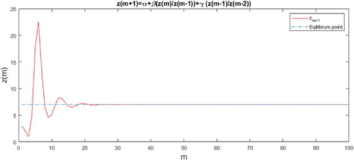
Example 2.1

Consider the equation (3) $z_{m+1}=\alpha +\text{β}\frac{z_m}{z_{m-1}}+\gamma \frac{z_{m-1}}{z_{m-2}}.$(3) We note that $f\left(u,v,w\right)=\alpha +\text{β}\frac{u}{v}+\gamma \frac{v}{w}$ was homogenous with degree zero. Then, by Theorem 2.1, the positive equilibrium point $\overline{z}=\alpha +\text{β}+\gamma$ was locally asymptotically stable if $\left|\gamma -\text{β}\right|<\alpha .$ For numerical example, let $\alpha =2,\text{β}=3,\gamma =2,z_{-2}=1,z_{-1}=2$ and $z_0=3$, see Figure 1.

Figure 1. The stable solution corresponding to difference Equations (3(3) $z_{m+1}=\alpha +\text{β}\frac{z_m}{z_{m-1}}+\gamma \frac{z_{m-1}}{z_{m-2}}.$(3) ).

3. Period two

In this section we gave a new strategy of studying periodic solutions of prime period two, namely in Theorems 3.1 and 3.2. One other important feature of this method is that no restriction of the coefficients of difference equations, i.e. they are arbitrary real numbers.

Theorem 3.1

Assume that k odd. Equation (1(1) $z_{m+1}=f\left(z_m,z_{m-1},\dots ,z_{m-k}\right),$(1) ) had a prime period two solution $\dots ,p,q,p,q,\dots .$ if and only if (4) $f\left(1,\tau ,\dots ,1,\tau \right)=\tau f\left(\tau ,1,\dots ,\tau ,1\right),$(4) where $\tau =p/q$.

Proof.

Assume that k odd and Equation (1(1) $z_{m+1}=f\left(z_m,z_{m-1},\dots ,z_{m-k}\right),$(1) ) had a prime period two solution $\dots ,p,q,p,q,\dots .$ Then $z_{m-1}=z_{m-3}=\cdots =z_{m-(k-2)}=z_{m-k}=p$. From Equation (1(1) $z_{m+1}=f\left(z_m,z_{m-1},\dots ,z_{m-k}\right),$(1) ), we got $\begin{array}{rl}p& =f\left(q,p,q,p,\dots ,q,p\right)=f\left(1,\tau ,\dots ,1,\tau \right),\\ q& =f\left(p,q,p,q,\dots ,p,q\right)=f\left(\tau ,1,\dots ,\tau ,1\right).\end{array}$ Since $\tau =p/q$, we obtain $0=p-\tau q=f\left(1,\tau ,\dots ,1,\tau \right)-\tau f\left(\tau ,1,\dots ,\tau ,1\right).$ On the other hand, let we have (4(4) $f\left(1,\tau ,\dots ,1,\tau \right)=\tau f\left(\tau ,1,\dots ,\tau ,1\right),$(4) ) holds. Now, we chose $\begin{array}{rl}{z}_{-2\mu }& =f\left(\tau ,1,\dots ,\tau ,1\right)\mathrm{a}\mathrm{n}\mathrm{d}{z}_{-2\mu +1}\\ & =f\left(1,\tau ,\dots ,1,\tau \right),\mu =0,1,\dots ,\left(k-1\right)/2,\end{array}$ where $\tau \in {\mathbb{R}}^{+}$. Hence, we see that $\begin{array}{rl}{z}_1& =f\left(z_0,z_{-l},\dots ,z_{-k}\right)\\ & =f\left(f\left(\tau ,1,\dots ,\tau ,1\right),f\left(1,\tau ,\dots ,1,\tau \right),\dots ,f\right.\\ & \left.\times \left(\tau ,1,\dots ,\tau ,1\right),f\left(1,\tau ,\dots ,1,\tau \right)\right)\\ & =f\left(f\left(\tau ,1,\dots ,\tau ,1\right),\tau f\left(\tau ,1,\dots ,\tau ,1\right),f\right.\\ & \times \left(\tau ,1,\dots ,\tau ,1\right),\dots ,\tau f\left(\tau ,1,\dots ,\tau ,1\right),\\ & \left.\times f\left(\tau ,1,\dots ,\tau ,1\right)\right)\\ & =f\left(1,\tau ,\dots ,1,\tau \right).\end{array}$ Similarly, we can proof that $z_2=f(1,\tau ,\dots ,1,\tau )$. Hence, it is followed by the induction that $\begin{array}{rl}{z}_{2n-1}& =f\left(\tau ,1,\dots ,\tau ,1\right)\mathrm{a}\mathrm{n}\mathrm{d}{z}_{2n}=f\left(1,\tau ,\dots ,1,\tau \right)\\ & \mathrm{f}\mathrm{o}\mathrm{r}\mathrm{a}\mathrm{l}\mathrm{l}n>0.\end{array}$ Therefore,Equation (1(1) $z_{m+1}=f\left(z_m,z_{m-1},\dots ,z_{m-k}\right),$(1) ) had a prime period two solution. Hence the proof is completed.

Theorem 3.2

Assume that k even. Equation (1(1) $z_{m+1}=f\left(z_m,z_{m-1},\dots ,z_{m-k}\right),$(1) ) had a prime period two solution $\dots ,p,q,p,q,\dots .$ if and only if (5) $f\left(1,\tau ,1\dots ,\tau ,1\right)=\tau f\left(\tau ,1,\tau \dots ,1,\tau \right),$(5) where $\tau =p/q$.

Proof.

The proof was similar to that of proof of Theorem 3.1 and hence is omitted.

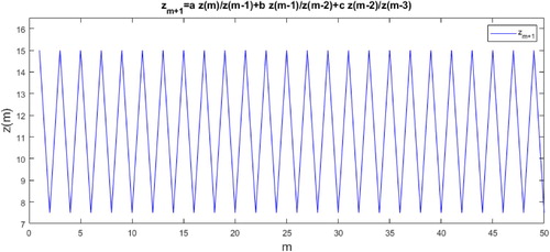
Example 3.1

Consider the difference equation (6) $z_{m+1}=a\frac{z_m}{z_{m-1}}+b\frac{z_{m-1}}{z_{m-2}}+c\frac{z_{m-2}}{z_{m-3}}.$(6) Using Theorem 3.1, Equation (6(6) $z_{m+1}=a\frac{z_m}{z_{m-1}}+b\frac{z_{m-1}}{z_{m-2}}+c\frac{z_{m-2}}{z_{m-3}}.$(6) ) had periodic solutions of prime period two if and only if $a\frac{1}{\tau }+b\tau +c\frac{1}{\tau }=\tau \left(a\tau +b\frac{1}{\tau }+c\tau \right)$ and so, $\left(1-\tau \right)\left((a+c)(1+\tau +{\tau }^2+)-b\tau \right)=0.$ Since $p\ne q$, we have $\tau \ne 1$, and hence (7) $\frac{a+c}{b}=\frac{\tau }{1+\tau +{\tau }^2}.$(7) Now, we have $\tau >0$, then the function $y\left(t\right)=(1+\tau +{\tau }^2)/\tau$ attends its minimum value on ${\mathbb{R}}^{+}$ at ${\tau }_0=1$ and $\underset{\tau \in {\mathbb{R}}^{+}}{min}y=y\left({\tau }_0\right)=3$, and so $\frac{1+\tau +{\tau }^2}{\tau }>\underset{\tau \in {\mathbb{R}}^{+}}{min}y=3\mathrm{f}\mathrm{o}\mathrm{r}\tau >0,\tau \ne 1,$ which with (7(7) $\frac{a+c}{b}=\frac{\tau }{1+\tau +{\tau }^2}.$(7) ) gives $3(a+c)>b$. For example, $a=2,b=3,c=2,$ $z_{-1}=15$ and $z_0=7.5$, see Figure 2.

Figure 2. Prime period two for Equation (6(6) $z_{m+1}=a\frac{z_m}{z_{m-1}}+b\frac{z_{m-1}}{z_{m-2}}+c\frac{z_{m-2}}{z_{m-3}}.$(6) ).

4. Oscillation of solutions

In this section we studied the oscillation behaviour of the solution for Equation (1(1) $z_{m+1}=f\left(z_m,z_{m-1},\dots ,z_{m-k}\right),$(1) ).

Theorem 4.1

Equation (1(1) $z_{m+1}=f\left(z_m,z_{m-1},\dots ,z_{m-k}\right),$(1) ) had oscillatory solution about $\overline{z}=f(1,1,\dots 1)$ if one of the following statements holds

1. $k\mathrm{o}\mathrm{d}\mathrm{d},f_{uj}>0\text{and}{f}_{ui}<0,fori=0,2,4,\dots ,k-1,j=1,3,5,\dots ,k$.

2. $k\mathrm{e}\mathrm{v}\mathrm{e}\mathrm{n}{f}_{uj}>0\text{and}{f}_{ui}<0,$ for $i=0,2,4,\dots ,k,j=1,3,5,\dots ,k-1$.

Proof.

We first prove case (1), case (2) follows in the same way. Let $\{z_n{\}}_{n=-k}^{\mathrm{\infty }}$ solution of Equation (1(1) $z_{m+1}=f\left(z_m,z_{m-1},\dots ,z_{m-k}\right),$(1) ) with initial data satisfy $z_{-2\eta }<\overline{z}\mathrm{a}\mathrm{n}\mathrm{d}{z}_{-2\eta +1}>\overline{z}\mathrm{f}\mathrm{o}\mathrm{r}\mathrm{a}\mathrm{l}\mathrm{l}\eta =1,\dots ,k/2.$ Since k odd, we have $z_{-l}>\overline{z}$. From Equation (1(1) $z_{m+1}=f\left(z_m,z_{m-1},\dots ,z_{m-k}\right),$(1) ), we obtain $\begin{array}{rl}{z}_1& =f\left(z_0,z_{-1},\dots ,z_{-k}\right)\\ & >f\left(\overline{z},z_{-1},\dots ,z_{-k}\right)\\ & >f\left(\overline{z},\overline{z},\dots ,\overline{z}\right)=\overline{z}\end{array}$

also, $\begin{array}{rl}{z}_2& =f\left(z_1,z_0,z_{-1},\dots ,z_{-k+1}\right)\\ & <f\left(\overline{z},z_0,z_{-1},\dots ,z_{-k+1}\right)\\ & <f\left(\overline{z},\overline{z},\dots ,\overline{z}\right)=\overline{z}.\end{array}$ Then, it was followed by the induction that $z_{2m}<\overline{z}\mathrm{a}\mathrm{n}\mathrm{d}{z}_{2m-1}>\overline{z}\mathrm{f}\mathrm{o}\mathrm{r}\mathrm{a}\mathrm{l}\mathrm{l}m\ge 1.$ Then, $\{z_n{\}}_{n=-k}^{\mathrm{\infty }}$ was oscillatory solution. Hence, the proof is completed.

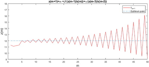
Example 4.1

Consider the equation (8) $z_{m+1}=\alpha +\text{β}\frac{z_{m-1}}{z_m}+\gamma \frac{z_{m-3}}{z_{m-2}}.$(8) We noted that k odd and (8(8) $z_{m+1}=\alpha +\text{β}\frac{z_{m-1}}{z_m}+\gamma \frac{z_{m-3}}{z_{m-2}}.$(8) ) was homogenous with degree zero and so, Then, by Theorem 4.1,Equation (8(8) $z_{m+1}=\alpha +\text{β}\frac{z_{m-1}}{z_m}+\gamma \frac{z_{m-3}}{z_{m-2}}.$(8) ) had oscillatory solution about $\overline{z}=\alpha +\text{β}+\gamma$. If $\alpha =5$ and $\text{β}=4,\gamma =3$, then Equation (8(8) $z_{m+1}=\alpha +\text{β}\frac{z_{m-1}}{z_m}+\gamma \frac{z_{m-3}}{z_{m-2}}.$(8) ) had oscillatory solution about $\overline{z}=12$ with initial data $z_{-3}=11.3,$ $z_{-2}=11.1$, $z_{-1}=11.22,$ $z_0=11.3$, see Figure 3.

Figure 3. Oscillation of solution for Equation (8(8) $z_{m+1}=\alpha +\text{β}\frac{z_{m-1}}{z_m}+\gamma \frac{z_{m-3}}{z_{m-2}}.$(8) ).

5. Applications

There were so many homogenous rational difference equations, which emerged from (1(1) $z_{m+1}=f\left(z_m,z_{m-1},\dots ,z_{m-k}\right),$(1) ). Here we gave only three applications of the homogenous rational difference Equation (1(1) $z_{m+1}=f\left(z_m,z_{m-1},\dots ,z_{m-k}\right),$(1) ), specifically we studied the stability and periodicity for these equations.

5.1. Application 1

Consider the equation (9) $z_{m+1}=a+b{\mathrm{e}}^{\left((z_{m-1}+z_{m-2})/z_m\right)}.$(9) We note that $f\left(u,v\right)=a+b{\mathrm{e}}^{(u+v)/w}$ was homogenous with degree zero.

Stability: By Theorem 2.1, the positive equilibrium point $\overline{z}=a+b{\mathrm{e}}^2$ was locally asymptotically stable if $\left|f_u\left(1,1,1\right)\right|+\left|f_v\left(1,1,1\right)\right|+\left|f_w\left(1,1,1\right)\right|<f\left(1,1,1\right)$ and hence $3b{\mathrm{e}}^2<a.$ For example a = 7, b = 0.2,$z_{-2}=8.4$, $z_{-1}=8.6$ and $z_0=8.7$, see Figure 4(a).

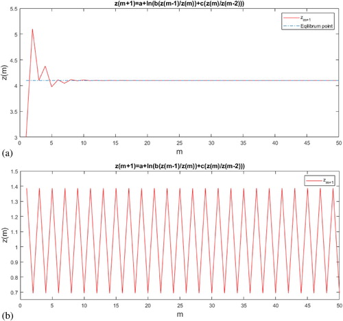
Figure 4. The stable and periodic solutions corresponding to difference Equation (9(9) $z_{m+1}=a+b{\mathrm{e}}^{\left((z_{m-1}+z_{m-2})/z_m\right)}.$(9) ), respectively.

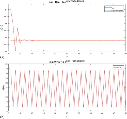
Periodicity: By using Theorem 3.2, if Equation (9(9) $z_{m+1}=a+b{\mathrm{e}}^{\left((z_{m-1}+z_{m-2})/z_m\right)}.$(9) ) had a prime period two solution, then (10) $a=b\left(\frac{\tau {\mathrm{e}}^{(\tau +1)/\tau }-{\mathrm{e}}^{\tau +1}}{1-\tau }\right).$(10) Now, we have that $\underset{\tau \in {\mathbb{R}}^{+}}{min}\left(\frac{\tau {\mathrm{e}}^{(\tau +1)/\tau }-{\mathrm{e}}^{\tau +1}}{1-\tau }\right)={\mathrm{e}}^2,$ which with (10(10) $a=b\left(\frac{\tau {\mathrm{e}}^{(\tau +1)/\tau }-{\mathrm{e}}^{\tau +1}}{1-\tau }\right).$(10) ) gives $a>b{\mathrm{e}}^2$. For example $a={\mathrm{e}}^3-2{\mathrm{e}}^{3/2},b=1,z_{-2}=2{\mathrm{e}}^3-{\mathrm{e}}^{3/2},z_{-1}={\mathrm{e}}^3-{\mathrm{e}}^{3/2}$. and $z_0=2{\mathrm{e}}^3-{\mathrm{e}}^{3/2}$, see Figure 4(b).

5.2. Application 2

Consider the equation (11) $z_{m+1}=a+\ln \left(b\frac{z_{m-1}}{z_m}+c\frac{z_m}{z_{m-2}}\right),$(11) where a, b and c were positive real numbers and $b\ge 1$. We noted that $f\left(u,v,w\right)=a+\ln \left(b\frac{u}{v}+c\frac{v}{w}\right)$ was homogenous with degree zero.

Stability: By Theorem 2.1, the positive equilibrium point $\overline{z}=a+\ln (b+c)$ was locally asymptotically stable if $\left|f_u\left(1,1,1\right)\right|+\left|f_v\left(1,1,1\right)\right|+\left|f_w\left(1,1,1\right)\right|<f\left(1,1,1\right)$ and hence $b+c+\mid b-c\mid <\left(a+\ln \left(b+c\right)\right)\ln \left(b+c\right).$ For example $a=3,b=1,c=2,z_{-2}=4.1,z_{-1}=5$ and $z_0=3$, see Figure 5(a).

Figure 5. The stable and periodic solutions corresponding to difference Equation (11(11) $z_{m+1}=a+\ln \left(b\frac{z_{m-1}}{z_m}+c\frac{z_m}{z_{m-2}}\right),$(11) ), respectively.

Periodicity: By using Theorem 3.2, if Equation (11(11) $z_{m+1}=a+\ln \left(b\frac{z_{m-1}}{z_m}+c\frac{z_m}{z_{m-2}}\right),$(11) ) had a prime period two solution, then $a=\frac{\tau \ln \left(b\frac{1}{\tau }+c\right)-\ln \left(b\tau +c\right)}{\left(1-\tau \right)}$ If $b=c,$ then (12) $a=\left[\frac{\tau \ln \tau }{\left(\tau -1\right)}+\ln \left(1+\tau \right)\right]-\ln b.$(12) Since $\tau >0$, we got $\underset{\tau \in {\mathbb{R}}^{+}}{max}\left[\frac{\tau \ln \tau }{\left(\tau -1\right)}-\ln \left(1+\tau \right)\right]\simeq 0.32,$ which with ( 12(12) $a=\left[\frac{\tau \ln \tau }{\left(\tau -1\right)}+\ln \left(1+\tau \right)\right]-\ln b.$(12) ) gives $a<0.32-\ln b$. For example $a=2\ln 2-\ln 3,b=c=1,z_{-2}=2\ln 2,z_{-1}=\ln 2$ and $z_0=2\ln 2$, see Figure 5(b).

5.3. Application 3

Consider the equation (13) $z_{m+1}=\alpha +{\left(\frac{a{z}_m+b{z}_{m-1}}{c{z}_m+d{z}_{m-1}}\right)}^{\gamma },$(13) where $\alpha ,a,b,c$ and d were positive real numbers and γ positive integer. We noted that $f\left(u,v\right)=\alpha +{\left(\frac{au+bv}{cu+dv}\right)}^{\gamma }$ was homogenous with degree zero.

Stability: By Theorem 2.1, the positive equilibrium point $\overline{z}=\alpha +((a+b)/(c+d){)}^{\gamma }$ was locally asymptotically stable if $\left|f_u\left(1,1\right)\right|+\left|f_v\left(1,1\right)\right|<f\left(1,1\right)$ and so, $\begin{array}{rl}& \left(2\gamma \left|ad-cb\right|-\left(a+b\right)\left(c+d\right)\right){\left(\frac{a+b}{c+d}\right)}^{\gamma }\\ & <\alpha \left(a+b\right)\left(c+d\right).\end{array}$ For example $\gamma =5,\alpha =2,a=2,b=1,c=3,d=2,z_{-1}=3$ and $z_0=4$, see Figure 6(a) (on the left).

Figure 6. The stable and periodic solutions corresponding to difference Equation (13(13) $z_{m+1}=\alpha +{\left(\frac{a{z}_m+b{z}_{m-1}}{c{z}_m+d{z}_{m-1}}\right)}^{\gamma },$(13) ), respectively.

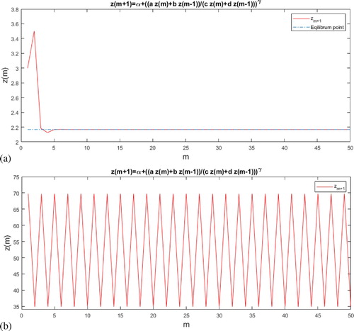
Periodicity: By using Theorem 3.1, if Equation (13(13) $z_{m+1}=\alpha +{\left(\frac{a{z}_m+b{z}_{m-1}}{c{z}_m+d{z}_{m-1}}\right)}^{\gamma },$(13) ) had a prime period two solution, then $\alpha =\frac{1}{1-\tau }\left[\tau {\left(\frac{a\tau +b}{c\tau +d}\right)}^{\gamma }-{\left(\frac{a+b\tau }{c+d\tau }\right)}^{\gamma }\right].$ For example $\gamma =3,\alpha =26.875,a=1,b=3,c=1,d=0.5,z_{-1}=69.75$ and $z_0=34.875$, see Figure 6(b).

6. Conclusions

A general class of difference equations is introduced in this work. Here, we summarize the main results of this research as follows.

1. The stability, periodicity and oscillation of the solution of these equations are studied.

2. An efficient method is considered to study periodic solution of period two without any restriction of the coefficients of difference equations.

3. This study included so many other equations even studied by other authors.

4. Three applications of these equations are given in order to support our analysis.

Thus we concluded that this study presented a new as well as strong motivation of difference equations.

Acknowledgments

The author thanks the editor and referees for their valuable comments and suggestions.

Disclosure statement

No potential conflict of interest was reported by the author.

ORCID

Mahmoud A. E. Abdelrahman  http://orcid.org/0000-0002-7351-2088

References

- Abdelrahman MAE, Moaaz O. Investigation of the new class of the nonlinear rational difference equations. Fund Res Dev Int. 2017;7(1):59–72.
- Abdelrahman MAE, Moaaz O. On the new class of the nonlinear difference equations. Electron J Math Anal Appl. 2018;6(1):117–125.
- Abdelrahman MAE, Chatzarakis GE, Li T, et al. On the difference equation xn+1=axn−l+bxn−k+f(xn−l,xn−k). Adv Differ Equ. 2018;2018:431. doi:10.1186/s13662-018-1880-8
- Abu-Saris RM, DeVault R. Global stability of yn+1=A+yn/yn−k. Appl Math Lett. 2003;16:173–178.
- Amleh AM, Grove EA, Georgiou DA, et al. On the recursive sequence xn+1=α+xn−1/xn. J Math Anal Appl. 1999;233:790–798.
- Berenhaut KS, Foley JD, Stevic S. The global attractivity of the rational difference equation yn=1+yn−k/yn−m. Proc Amer Math Soc. 2007;135:1133–1140.
- Berenhaut KS, Stevic S. The behaviour of the positive solutions of the difference equation xn=A+(xn−2xn−1)p. J Differ Equ Appl. 2006;12(9):909–918.
- Border KC. Eulers theorem for homogeneous functions. Available from: http://www.hss.caltech.edu/kcb/Ec121a/Notes/EulerHomogeneity.pdf, 23 July 2009.
- Devault R, Ladas G, Schultz SW. On the recursive sequence xn+1=Axn+1xn−2. Proc Amer Math Soc. 1998;126:3257–3262.
- Devault R, Kent C, Kosmala W. On the recursive sequence xn+1=p+xn−kxn. J Differ Equ Appl. 2003;9(8):721–730.
- Devault R, Schultz SW. On the dynamics of xn+1=βxn+γxn−1Bxn+Dxn−2. Commun Appl Nonlinear Anal. 2005;12:35–40.
- Elabbasy EM, El-Metwally H, Elsayed EM. On the difference equation xn+1=αxn−l+βxn−kAxn−l+Bxn−k. Acta Math Vietnam. 2008;33(1):85–94.
- Elsayed EM. New method to obtain periodic solutions of period two and three of a rational difference equation. Nonlinear Dyn. 2015;79:241–250.
- Hamza AE. On the recursive sequence xn+1=α+xn−1xn. J Math Anal Appl. 0000;322(6):668–674.
- Kalabusic S, Kulenovic MRS. On the recursive sequence xn+1=γxn−1+δxn−2Cxn−1+Dxn−2. J Differ Equ Appl. 2003;9(8):701–720.
- Kulenovic MRS, Ladas G, Sizer WS. On the dynamics of xn+1=αxn+βxn−1γxn+δxn−1. Math Sci Res Hot-Line. 1998;2(5):1–16.
- Khuong VV. On the positive nonoscillatory solution of the difference equations xn+1=α+(xn−k/xn−m)p. Appl Math J Chin Univ. 2008;24:45–48.
- Kocic VL, Ladas G. Global behavior of nonlinear difference equations of higher order with applications. Dordrecht: Kluwer Academic; 1993.
- Kulenovic MRS, Ladas G. Dynamics of second order rational difference equations. London: Chapman & Hall/CRC; 2002.
- Moaaz O, Abdelrahman MAE. Behaviour of the new class of the rational difference equations. Electron J Math Anal Appl. 2016;4(2):129–138.
- Moaaz O. Comment on ‘New method to obtain periodic solutions of period two and three of a rational difference equation’ [Nonlinear Dyn 79:241–250]. Nonlinear Dyn. 2016.
- Moaaz O, Abdelrahman MAE. On the class of the rational difference equations. Int J Adv Math. 2017;4:46–55.
- Ocalan O. Dynamics of the difference equation xn+1=p+xn−kxn with a period-two coefficient. Appl Math Comput. 2014;228:31–37.
- Saleh M, Aloqeili M. On the rational difference equation xn+1=A+xn−kxn. Appl Math Comput. 2005;171(2):862–869.
- Stevic S. On the recursive sequence xn+1=α+xn−1pxnp. J Appl Math Comput. 2005;18:229–234.
- Stevic S, Kent C, Berenaut S. A note on positive nonoscillatory solutions of the differential equation xn+1=α+xn−1pxnp. J Differ Equ Appl. 2006;12:495–499.
- Sun T, Xi H. On convergence of the solutions of the difference equation xn+1=1+xn−1xn. J Math Anal Appl. 2007;325(2):1491–1494.
- Yan XX, Li WT, Zhao Z. On the recursive sequence xn+1=α−(xnxn−1). J Appl Math Comput. 2005;17(1):269–282.