Existence of a finite multiplicative search plan with random distances and velocities to find a d-dimensional Brownian target

Abstract

We present the existence of a finite search plan to find Brownian target on the d-space by using d-searchers. Each searcher moves continuously in both directions of the origin (starting point) of the line (field of its search) with random distances and velocities. We express theses distances and velocities with independent random variables with known probability density functions (PDFs). We present more analysis about the density of the random distances in our model by using Fourier–Laplace representation. This analysis will provide us with the conditions that make the expected value of the first meeting time between the target and one of the searchers finite.

Keywords:

• Random search
• Brownian motion
• Fourier–Laplace representation

Mathematics Subject Classifications:

• 37A50
• 60K30

1. Introduction

The searching techniques for a randomly moving target on the space has many applicabilitions in our life, for example, finding the charged particles in plasmas that move in the space with d-dimensional Brownian motion. In all searching techniques, the searchers move with known distances and velocities. If the search space is a line, then the searcher aims to detect the target in the right or left part of the starting point, where the searcher can change its direction without losing any time. Most of the techniques that have been studied for the line deal with deterministic distances and velocities, see [1–7]. On the plane, Mohamed and El-Hadidy [8, 9] and El-Hadidy [10] presented more interesting search strategies with deterministic distance and regular fixed velocity to find the two-dimensional randomly moving targets. On the space, El-Hadidy and colleagues [11–16] studied different techniques with deterministic distances and velocities by using multiple searchers. The main objective of these earlier works is to obtain the conditions that make the first meeting time between one of the searchers and the moving target finite. On the other hand, when the target is located, some earlier works discussed many different search strategies with deterministic distances and velocities to find this target in minimum time on the line, plane and space , such as [17–25].

In this work, we need to find the condition that makes the expected value of the first meeting time between one of the d searchers and the d-dimensional Brownian target finite. We consider that the searchers have a nonstop random motion with random distances and velocities where there are no restrictions on the searcher's movement. We use the Fourier–Laplace transform to give an analytical expression for the random distance density functions that the searchers should do them with random velocities.

This paper is organized as follows. Section 1 gives an analytical expression for the density of random distances and velocities. In Section 2, we describe the searching problem based on this analytical expression. The condition that shows the existence of our search strategy is discussed in Section 3. Finally, the paper concludes with a discussion of the results.

2. Formulation of the model

We consider that the searching process starts from the origin of the d-space by d-searchers. These searchers move continuously along d-line. Each searcher moves in both directions of its origin. On the line $L_i,i=1,2,\dots ,d,$ we consider the searcher $S_i,i=1,2,\dots ,d$ has the following strategy: start at $h_{i0}=0$ to cut a random distance $h_{i1}$ with a certain random velocity $v_i$ on the left (right) part of $L_i$. After that, turn back to $h_{i0}$ and go a distance $h_{i2}$ to search the other right (left) part of $h_{i0}$. Retrace the steps again to search the left (right) part of $h_{i1}$ as far as $h_{i3}$ and so on. Now, the searcher changes the direction and magnitude of its velocity (this velocity can have positive as well as negative values to include the direction of searcher motion) to another random point with random distance ${\tilde{h}}_i$ and continues the search for another random distance. For our model, we assume $g_i\left(v_i\right)$ and $f_i\left(h_i\right),i=1,2,\dots ,d,$ to be Probability Densities Functions (PDFs) of the basic and independent random distances and the velocities variables, respectively. 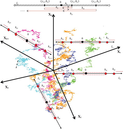Each one of these PDFs is normalized to one, where ${\int }_{-\mathrm{\infty }}^{+\mathrm{\infty }}$ $g_i\left(v_i\right)\mathrm{d}{v}_i=1,{\int }_0^{+\mathrm{\infty }}$$f_i\left(h_i\right)\mathrm{d}{h}_i=1$ and $g_i\left(v_i\right)=g_i(-v_i)$ (the velocity distribution is symmetric) for all $i=1,2,\dots ,d,$ then there is no bias in the search model. In our model, we let the searcher $S_i$ changes its direction on $L_i$ at the random points $y_i$ as in Figure 1. Let $l_{i0}\left(y_i\right),i=1,2,\dots ,d,$ be the PDFs for the initial distribution of the searchers at the random points $y_1,y_2,\dots ,y_d,$ respectively, then we aim to determine the evolution of the density functions $l_i(y_i,h_i),i=1,2,\dots ,d,$ of the locations for the searchers $S_i,i=1,2,\dots ,d,$ respectively.

Figure 1. The search strategy $\phi \left(t\right)$ for meeting a d-dimensional Brownian target.

At time t, let PDFs ${\varsigma }_i(y_i,h_i),i=1,2,\dots ,d,$ represent the changes of the searchers' velocities at the position $[y_i,y_i+d{y}_i]$ and refer to it as the frequency of velocity changes: (1) $\begin{array}{rl}{\varsigma }_i(y_i,h_i)& ={\int }_{-\mathrm{\infty }}^{+\mathrm{\infty }}{\int }_0^{h_i}{\varsigma }_i(y_i-v_{i}t,h_i-{\tilde{h}}_i)g_i\left(v_i\right)f_i\left({\tilde{h}}_i\right)\\ & \times \mathrm{d}{\tilde{h}}_i\mathrm{d}{v}_i+l_{i0}\left(y_i\right){\delta }_i\left(h_i\right).\end{array}$(1) After doing the random distance ${\tilde{h}}_i$ at time t, each searcher $S_i$ changes its velocity $v_i$ at the point $(y_i,h_i)$, distance $h_i-{\tilde{h}}_i$ and position $y_i-v_{i}t$. In addition, we let $g_i\left(v_i\right)f_i\left({\tilde{h}}_i\right)$ to be the probability density function of a certain velocity $v_i$. Thus, we can integrate the first term on the right-hand side of (1(1) $\begin{array}{rl}{\varsigma }_i(y_i,h_i)& ={\int }_{-\mathrm{\infty }}^{+\mathrm{\infty }}{\int }_0^{h_i}{\varsigma }_i(y_i-v_{i}t,h_i-{\tilde{h}}_i)g_i\left(v_i\right)f_i\left({\tilde{h}}_i\right)\\ & \times \mathrm{d}{\tilde{h}}_i\mathrm{d}{v}_i+l_{i0}\left(y_i\right){\delta }_i\left(h_i\right).\end{array}$(1) ), over all these events. In the last term of (1(1) $\begin{array}{rl}{\varsigma }_i(y_i,h_i)& ={\int }_{-\mathrm{\infty }}^{+\mathrm{\infty }}{\int }_0^{h_i}{\varsigma }_i(y_i-v_{i}t,h_i-{\tilde{h}}_i)g_i\left(v_i\right)f_i\left({\tilde{h}}_i\right)\\ & \times \mathrm{d}{\tilde{h}}_i\mathrm{d}{v}_i+l_{i0}\left(y_i\right){\delta }_i\left(h_i\right).\end{array}$(1) ), $l_{i0}(y_i,h_{i0}=0)=l_{i0}\left(y_i\right)$, and the velocities are changed at $h_{i0}=0$, then ${\delta }_i\left(t\right)$ will become an impulse function. By using the changes in the frequencies of the velocities, we can express $l_i(y_i,h_i)$ with the following: (2) $\begin{array}{rl}{l}_i(y_i,h_i)& ={\int }_{-\mathrm{\infty }}^{+\mathrm{\infty }}{\int }_0^{h_i}{\varsigma }_i(y_i-v_{i}t,h_i-{\tilde{h}}_i)\\ & \times g_i\left(v_i\right){\acute{f}}_i\left({\tilde{h}}_i\right)\mathrm{d}{\tilde{h}}_i\mathrm{d}{v}_i,\end{array}$(2) where ${\acute{f}}_i\left({\tilde{h}}_i\right)=1-{\int }_0^{{\tilde{h}}_i}{f}_i\left({\tilde{h}}_i^{/}\right)\mathrm{d}{\tilde{h}}_i^{/}$ is the PDF of nonchange velocity until the distance ${\tilde{h}}_i$. As a result of velocities changes, ${\varsigma }_i(y_i-v_{i}t,h_i-{\tilde{h}}_i)$. ${\acute{f}}_i\left({\tilde{h}}_i\right)$ shows that $S_i$ does not choose another velocity before passing the point $(y_i,h_i)$. Now, the motion of $S_i$ on the line $L_i$ with a given initial density and the two PDFs for the distances and velocities is described by Equations (1(1) $\begin{array}{rl}{\varsigma }_i(y_i,h_i)& ={\int }_{-\mathrm{\infty }}^{+\mathrm{\infty }}{\int }_0^{h_i}{\varsigma }_i(y_i-v_{i}t,h_i-{\tilde{h}}_i)g_i\left(v_i\right)f_i\left({\tilde{h}}_i\right)\\ & \times \mathrm{d}{\tilde{h}}_i\mathrm{d}{v}_i+l_{i0}\left(y_i\right){\delta }_i\left(h_i\right).\end{array}$(1) ) and (2(2) $\begin{array}{rl}{l}_i(y_i,h_i)& ={\int }_{-\mathrm{\infty }}^{+\mathrm{\infty }}{\int }_0^{h_i}{\varsigma }_i(y_i-v_{i}t,h_i-{\tilde{h}}_i)\\ & \times g_i\left(v_i\right){\acute{f}}_i\left({\tilde{h}}_i\right)\mathrm{d}{\tilde{h}}_i\mathrm{d}{v}_i,\end{array}$(2) ) which can be solved analytically. Hence, we aim to find the frequency of velocity changes ${\varsigma }_i(y_i,h_i)$ and then substitute with result (2(2) $\begin{array}{rl}{l}_i(y_i,h_i)& ={\int }_{-\mathrm{\infty }}^{+\mathrm{\infty }}{\int }_0^{h_i}{\varsigma }_i(y_i-v_{i}t,h_i-{\tilde{h}}_i)\\ & \times g_i\left(v_i\right){\acute{f}}_i\left({\tilde{h}}_i\right)\mathrm{d}{\tilde{h}}_i\mathrm{d}{v}_i,\end{array}$(2) ).

According to the shift property of the Fourier transformation and by applying it with respect to the spatial coordinate in (1(1) $\begin{array}{rl}{\varsigma }_i(y_i,h_i)& ={\int }_{-\mathrm{\infty }}^{+\mathrm{\infty }}{\int }_0^{h_i}{\varsigma }_i(y_i-v_{i}t,h_i-{\tilde{h}}_i)g_i\left(v_i\right)f_i\left({\tilde{h}}_i\right)\\ & \times \mathrm{d}{\tilde{h}}_i\mathrm{d}{v}_i+l_{i0}\left(y_i\right){\delta }_i\left(h_i\right).\end{array}$(1) ), we get the factor ${\mathrm{e}}^{-jk{v}_i{\tilde{h}}_i},$ $j=\sqrt{-1},$ appears under the integral. If we integrate with respect to $v_i,$ then we get the Fourier transformation of $g_i\left(v_i\right)$ with a reciprocal velocity $k{\tilde{h}}_i$. The Fourier transformation of (1(1) $\begin{array}{rl}{\varsigma }_i(y_i,h_i)& ={\int }_{-\mathrm{\infty }}^{+\mathrm{\infty }}{\int }_0^{h_i}{\varsigma }_i(y_i-v_{i}t,h_i-{\tilde{h}}_i)g_i\left(v_i\right)f_i\left({\tilde{h}}_i\right)\\ & \times \mathrm{d}{\tilde{h}}_i\mathrm{d}{v}_i+l_{i0}\left(y_i\right){\delta }_i\left(h_i\right).\end{array}$(1) ) can be given by (3) ${\varsigma }_{ik}\left(h_i\right)={\int }_0^{h_i}{\varsigma }_i(h_i-{\tilde{h}}_i)g_{ik{\tilde{h}}_i}{f}_i\left({\tilde{h}}_i\right)\mathrm{d}{\tilde{h}}_i\mathrm{d}{v}_i+l_{i0,k}{\delta }_i\left(h_i\right),$(3) (see [26]) where the indices k and $k{\tilde{h}}_i$ denote the Fourier components. Now, by applying the Laplace transformation with respect to t and by using convolution property, we get (4) ${\varsigma }_{ik,\mathcal{L}}={\varsigma }_{ik,\mathcal{L}}{\left[g_{ik{\tilde{h}}_i}{f}_i\left({\tilde{h}}_i\right)\right]}_{\mathcal{L}}+l_{i0,k},$(4) where $\mathcal{L}\left[{\delta }_i\right(h_i\left)\right]=1,i=1,2,\dots ,n,$ and $\mathcal{L}$ denotes the Laplace component. Thus, the frequency velocity changes in the Fourier–Laplace domain, ${\varsigma }_{ik,\mathcal{L}}$, is given by (5) ${\varsigma }_{ik,\mathcal{L}}=\frac{l_{i0,k}}{1-{\left[g_{ik{\tilde{h}}_i}{f}_i\left({\tilde{h}}_i\right)\right]}_{\mathcal{L}}}.$(5) By the same method, the Fourier–Laplace transformation of the two equations (2(2) $\begin{array}{rl}{l}_i(y_i,h_i)& ={\int }_{-\mathrm{\infty }}^{+\mathrm{\infty }}{\int }_0^{h_i}{\varsigma }_i(y_i-v_{i}t,h_i-{\tilde{h}}_i)\\ & \times g_i\left(v_i\right){\acute{f}}_i\left({\tilde{h}}_i\right)\mathrm{d}{\tilde{h}}_i\mathrm{d}{v}_i,\end{array}$(2) ) and (5(5) ${\varsigma }_{ik,\mathcal{L}}=\frac{l_{i0,k}}{1-{\left[g_{ik{\tilde{h}}_i}{f}_i\left({\tilde{h}}_i\right)\right]}_{\mathcal{L}}}.$(5) ) together gives: (6) $l_{ik,\mathcal{L}}=\frac{{\left[g_{ik{\tilde{h}}_i}{\acute{f}}_i\left({\tilde{h}}_i\right)\right]}_{\mathcal{L}}{l}_{i0,k}}{1-{\left[g_{ik{\tilde{h}}_i}{f}_i\left({\tilde{h}}_i\right)\right]}_{\mathcal{L}}}.$(6) As in [27], the Fourier–Laplace representation of the exponential functions is more suitable to get our analytical expression. Thus, by using the spatial coordinate in (1(1) $\begin{array}{rl}{\varsigma }_i(y_i,h_i)& ={\int }_{-\mathrm{\infty }}^{+\mathrm{\infty }}{\int }_0^{h_i}{\varsigma }_i(y_i-v_{i}t,h_i-{\tilde{h}}_i)g_i\left(v_i\right)f_i\left({\tilde{h}}_i\right)\\ & \times \mathrm{d}{\tilde{h}}_i\mathrm{d}{v}_i+l_{i0}\left(y_i\right){\delta }_i\left(h_i\right).\end{array}$(1) ), our analytical expression for $S_i,i=1,2,\dots ,n,$ densities $g_i\left(v_i\right)$ and $f_i\left(h_i\right)$ (nonnegative locally integrable functions on $\mathbb{R}$) with random distances and velocities is sufficient to prove the existence of finiteness for these kinds of search strategies.

2.1. The searching problem

We consider a d-dimensional Brownian target that moves in ${\mathbb{R}}^d$ with families of independent random variables $\left(B_1\right(t),B_2(t),\dots ,B_d(t\left)\right),$ $t\ge 0$. These independent processes have a drift vector $[{\mu }_1,{\mu }_2,\dots ,{\mu }_d]$ and a covariance matrix Σ that is a diagonal matrix with only non-zero ${\sigma }_i^2,$ $i=1,2,\dots ,d$. The initial position of the target has a known probability distribution.

Let $\phi \left(t\right)=\left({\phi }_1\right(t),{\phi }_2(t),\dots ,{\phi }_n(t\left)\right)$ be a combination of vectors of continuous functions, where ${\phi }_i\left(t\right)=\left[{\phi }_{i1}\right(t),{\phi }_{i2}(t),\dots ,{\phi }_{id}(t\left)\right]$ with random speed $v_i$, and it is given by ${\phi }_i\left(t\right):{\mathbb{R}}^{d+}⟶\mathbb{R}$, $i=1,2,\dots ,d$. These functions are considered as the search strategies of the d-searchers $S_i,$ $i=1,2,\dots ,d,$ where (7) $\begin{array}{rl}& \left|{\phi }_i\left(t_1\right)-{\phi }_i\left(t_2\right)\right|<{\varsigma }_{ik,\mathcal{L}}\left|t_1-t_2\right|\\ & \mathrm{f}\mathrm{o}\mathrm{r}\mathrm{a}\mathrm{l}\mathrm{l}{t}_1,t_2\in {\mathbb{R}}^{+},{\phi }_i\left(0\right)=0\mathrm{a}\mathrm{n}\mathrm{d}i=1,2,\dots ,d.\end{array}$(7) Let ${\tau }_{\phi }\in {\mathbb{R}}^{+}$ be a random variable which represents the first meeting time between one of the searchers and the target. It is defined by ${\tau }_{\phi }=\left\{\begin{array}{l}inf\{t:\mathrm{e}\mathrm{i}\mathrm{t}\mathrm{h}\mathrm{e}\mathrm{r}\mathrm{o}\mathrm{n}\mathrm{e}\mathrm{o}\mathrm{f}{\phi }_i(t)\\ =\overrightarrow{X_0}+B\left(t\right),i=1,2,\dots ,n\},\\ \mathrm{\infty },\mathrm{i}\mathrm{f}\mathrm{t}\mathrm{h}\mathrm{e}\mathrm{s}\mathrm{e}\mathrm{t}\mathrm{i}\mathrm{s}\mathrm{e}\mathrm{m}\mathrm{p}\mathrm{t}\mathrm{y},\end{array}\right.$ where $\overrightarrow{X_0}=[X_{10},X_{20},\dots ,X_{d0}]$ is a vector of random variables that is independent of $B\left(t\right)=\left(B_1\right(t),B_2(t),\dots ,B_d(t\left)\right),$ $t\ge 0$ and represents the initial position of the target in ${\mathbb{R}}^d$. For each searcher $S_i,i=1,2,\dots ,d,$ we consider the set of all search strategies that satisfies (7(7) $\begin{array}{rl}& \left|{\phi }_i\left(t_1\right)-{\phi }_i\left(t_2\right)\right|<{\varsigma }_{ik,\mathcal{L}}\left|t_1-t_2\right|\\ & \mathrm{f}\mathrm{o}\mathrm{r}\mathrm{a}\mathrm{l}\mathrm{l}{t}_1,t_2\in {\mathbb{R}}^{+},{\phi }_i\left(0\right)=0\mathrm{a}\mathrm{n}\mathrm{d}i=1,2,\dots ,d.\end{array}$(7) ) and with a speed (5(5) ${\varsigma }_{ik,\mathcal{L}}=\frac{l_{i0,k}}{1-{\left[g_{ik{\tilde{h}}_i}{f}_i\left({\tilde{h}}_i\right)\right]}_{\mathcal{L}}}.$(5) ) be ${\phi }_{{\varsigma }_{ik,\mathcal{L}}}\left(t\right)$. We seek for the condition that gives finiteness of the expected value of ${\tau }_{\phi }$ (i.e. $E_{{\tau }_{\phi }}<\mathrm{\infty }$), where $\phi \left(t\right)\in \mathrm{\Phi }\left(t\right)$ (is the class of all of search strategies) and $\mathrm{\Phi }\left(t\right)=\left\{\phi \right(t);\phi (t)\in {\mathrm{\Phi }}_{{\varsigma }_{ik,\mathcal{L}}}(t\left)\right\}$.

3. Existence of finiteness

At time t on the line $L_i,$ the searcher $S_i$ will become at the random point $y_{ij}$ after cutting the distance $h_{ij},i=1,2,\dots ,d;j=i,2,\dots$ (see Figure 1). Thus, we define the sequences: $\{G_{ij}{\}}_{i=1,2,\dots ,d;j\ge 0}$ and $\{h_{ij}{\}}_{i=1,2,\dots ,d;j\ge 0}$ such that $h_{ij}=(-1{)}^{j+1}{c}_i[G_{ij}+1+(-1{)}^{j+1}]$ and (11(11) $\frac{{\int }_0^{G_{ij}}{\tilde{h}}_i{l}_{ik,\mathcal{L}}\mathrm{d}{\tilde{h}}_i}{{\int }_{-\mathrm{\infty }}^{+\mathrm{\infty }}{v}_i{\varsigma }_{ik,\mathcal{L}}\mathrm{d}{v}_i}\le t\le \frac{{\int }_0^{G_{i(j+1)}}{\tilde{h}}_i{l}_{ik,\mathcal{L}}\mathrm{d}{\tilde{h}}_i}{{\int }_{-\mathrm{\infty }}^{+\mathrm{\infty }}{v}_i{\varsigma }_{ik,\mathcal{L}}\mathrm{d}{v}_i},$(11) ) satisfied, where $c_i$ is constant ($>0$), $G_{ij}={\lambda }_i({\theta }_i^j-1)$ and ${\theta }_i^j>1,$ ${\lambda }_i>0$. By using (6(6) $l_{ik,\mathcal{L}}=\frac{{\left[g_{ik{\tilde{h}}_i}{\acute{f}}_i\left({\tilde{h}}_i\right)\right]}_{\mathcal{L}}{l}_{i0,k}}{1-{\left[g_{ik{\tilde{h}}_i}{f}_i\left({\tilde{h}}_i\right)\right]}_{\mathcal{L}}}.$(6) ), we can get the expected value of the random distance $h_{ij}$ as follows: (8) $E\left(h_{ij}\right)={\int }_0^{G_{ij}}{\tilde{h}}_i{l}_{ik,\mathcal{L}}\mathrm{d}{\tilde{h}}_i.$(8) By using (5(5) ${\varsigma }_{ik,\mathcal{L}}=\frac{l_{i0,k}}{1-{\left[g_{ik{\tilde{h}}_i}{f}_i\left({\tilde{h}}_i\right)\right]}_{\mathcal{L}}}.$(5) ), we obtain (9) $E\left(v_i\right)={\int }_{-\mathrm{\infty }}^{+\mathrm{\infty }}{v}_i{\varsigma }_{ik,\mathcal{L}}\mathrm{d}{v}_i.$(9) Consequently, from (8(8) $E\left(h_{ij}\right)={\int }_0^{G_{ij}}{\tilde{h}}_i{l}_{ik,\mathcal{L}}\mathrm{d}{\tilde{h}}_i.$(8) ) and (9(9) $E\left(v_i\right)={\int }_{-\mathrm{\infty }}^{+\mathrm{\infty }}{v}_i{\varsigma }_{ik,\mathcal{L}}\mathrm{d}{v}_i.$(9) ), the expected value of the searching time to search $h_{ij}$ is (10) $E\left(T_{ij}\right)\le \frac{{\int }_0^{G_{ij}}{\tilde{h}}_i{l}_{ik,\mathcal{L}}\mathrm{d}{\tilde{h}}_i}{{\int }_{-\mathrm{\infty }}^{+\mathrm{\infty }}{v}_i{\varsigma }_{ik,\mathcal{L}}\mathrm{d}{v}_i}.$(10) When (11) $\frac{{\int }_0^{G_{ij}}{\tilde{h}}_i{l}_{ik,\mathcal{L}}\mathrm{d}{\tilde{h}}_i}{{\int }_{-\mathrm{\infty }}^{+\mathrm{\infty }}{v}_i{\varsigma }_{ik,\mathcal{L}}\mathrm{d}{v}_i}\le t\le \frac{{\int }_0^{G_{i(j+1)}}{\tilde{h}}_i{l}_{ik,\mathcal{L}}\mathrm{d}{\tilde{h}}_i}{{\int }_{-\mathrm{\infty }}^{+\mathrm{\infty }}{v}_i{\varsigma }_{ik,\mathcal{L}}\mathrm{d}{v}_i},$(11) for all $t\in {\mathbb{R}}^{+}$, we have ${\phi }_i\left(t\right)=h_{ij}+(-1{)}^j[t-G_{ij}]$, where $h_{ij}$ is different from one searcher to another. There are very large numbers of events such that the first meeting between one of the searchers and the target may be done on the space. Now, we should turn into a new space called a probability space. Let the random variables that represent the target position are defined on a probability space $(\mathrm{\Omega },\varnothing ,\gamma )$, where Ω is the set of all possible meeting points, $\varnothing$ is the sigma algebra on these points and the location of the target at any time can be described by the probability measure γ. The following theorems contribute to the achievement of an existential search strategies. They help us to minimize $E_{{\tau }_{\phi }}$.

Theorem 3.1

Let $\phi \left(t\right)=\left({\phi }_1\right(t),{\phi }_2(t),\dots ,{\phi }_n(t\left)\right)$ be a combination of vectors of continuous functions, where ${\phi }_i\left(t\right)=\left[{\phi }_{i1}\right(t),{\phi }_{i2}(t),\dots ,{\phi }_{id}(t\left)\right]$ with random speed $v_i$. Then $E_{{\tau }_{\phi }}$ is finite if (12) $\begin{array}{rl}& \sum _{i=1}^d\sum _{j=0}^{\mathrm{\infty }}\prod _{u=1}^d\left[{\int }_0^{\mathrm{\infty }}p\left({\psi }_i{(}^{u}E\right(T_{i(2j-1)}\left)\right)>-x_{iju}\left)\gamma \right(\mathrm{d}{x}_{iju})\right.\\ & \left.+{\int }_{-\mathrm{\infty }}^{0}p\left({\tilde{\psi }}_i{(}^{u}E\right(T_{i\left(2j\right)}\left)\right)<-x_{iju}\left)\gamma \right(\mathrm{d}{x}_{iju})\right]\end{array}$(12) is finite.

Proof.

For each line $L_i,i=1,2,\dots ,d,$ if we consider ${\tilde{\psi }}_i\left(E\right(T_{2ij}\left)\right)=B_i\left(E\right(T_{2ij}\left)\right)+c_{i}E\left(T_{2ij}\right)$, ${\psi }_i\left(E\right(T_{i(2j+1)}\left)\right)=B_i\left(E\right(T_{i(2j+1)}\left)\right)-c_{i}E\left(T_{i(2j+1)}\right)$ and apply the same method in [28], then we have $B_i\left(E\right(T_{2ij}\left)\right)-\left(\frac{{\int }_0^{G_{2ij}}{\tilde{h}}_i{l}_{ik,\mathcal{L}}\mathrm{d}{\tilde{h}}_i}{{\int }_{-\mathrm{\infty }}^{+\mathrm{\infty }}{v}_i{\varsigma }_{ik,\mathcal{L}}\mathrm{d}{v}_i}\right)<-X_{0j}=x_{ij},$ then $B_i\left(E\right(T_{2ij}\left)\right)-(-1{)}^{\begin{array}{c}2j+1\end{array}}{c}_i[E\left(T_{2ij}\right)+1+(-1{)}^{2j+1}]<-x_{iju}.$ This gives $\begin{array}{rl}& B_i\left(E\right(T_{2ij}\left)\right)+c_i\left[E\right(T_{2ij})+1+(-1{)}^{2j+1}]\\ & =B_i\left(E\right(T_{2ij}\left)\right)+c_i\left[E\right(T_{2ij}\left)\right]+c_i[1+(-1{)}^{2j+1}]\\ & ={\tilde{\psi }}_i\left(E\right(T_{2ij}\left)\right)<-(x_{iju}+c_i[1+(-1{)}^{2j+1}]),\end{array}$ then ${\tilde{\psi }}_i\left(E\right(T_{2ij}\left)\right)<-x_{iju}$. By the same method and by using the notation ${\psi }_i\left(E\right(T_{i(2j+1)}\left)\right)=B_i\left(E\right(T_{i(2j+1)}\left)\right)-c_{i}E\left(T_{i(2j+1)}\right),$ we obtain ${\psi }_i\left(E\right(T_{2i(j+1)}\left)\right)>-x_{iju}$.

Since the events ${\tau }_{{\phi }_i}>t,$ $i=1,2,\dots ,d,$ are mutually exclusive events, then $p({\tau }_{\phi }>t)=p({\tau }_{{\phi }_1}>t$ or ${\tau }_{{\phi }_2}>t$ or ···  or ${\tau }_{{\phi }_n}>t)=\sum _{i=1}^{n}p({\tau }_{{\phi }_i}>t)$. Thus, for any $i=1,2,\dots ,d$ and $j=1,2,\dots ,$ we get $\begin{array}{rl}& p({\tau }_{\phi }>E(T_{i(2j+1)}\left)\right)\\ & \le {\int }_0^{\mathrm{\infty }}\cdots {\int }_0^{\mathrm{\infty }}{\int }_0^{\mathrm{\infty }}p\left({\psi }_1{(}^{1}E\right(T_{i(2j+1)}\left)\right)\\ & >-x_{ij1},{\psi }_2{(}^{2}E\left(T_{i(2j+1)}\right))>-x_{ij2}),\dots ,\\ & {\psi }_d{(}^{d}E\left(T_{i(2j+1)}\right))>-x_{ijd})\gamma \left(\mathrm{d}{x}_{ij1}\right)\gamma \left(\mathrm{d}{x}_{ij2}\right)\cdots \gamma \left(\mathrm{d}{x}_{ijd}\right)\\ & +{\int }_{-\mathrm{\infty }}^0\cdots {\int }_0^{\mathrm{\infty }}{\int }_0^{\mathrm{\infty }}p\left({\psi }_1{(}^{1}E\right(T_{i(2j+1)}\left)\right)\\ & >-x_{ij1},{\psi }_2{(}^{2}E\left(T_{i(2j+1)}\right))>-x_{ij2}),\dots ,\\ & {\tilde{\psi }}_d{(}^{d}E\left(T_{i\left(2j\right)}\right))<-x_{ijd})\gamma \left(\mathrm{d}{x}_{ij1}\right)\gamma \left(\mathrm{d}{x}_{ij2}\right)\cdots \gamma \left(\mathrm{d}{x}_{ijd}\right)\\ & +{\int }_{-\mathrm{\infty }}^0\cdots {\int }_{-\mathrm{\infty }}^0{\int }_0^{\mathrm{\infty }}p\left({\psi }_1{(}^{1}E\right(T_{i(2j+1)}\left)\right)\\ & >-x_{ij1},{\tilde{\psi }}_2{(}^{2}E\left(T_{i\left(2j\right)}\right))<-x_{ij2}),\dots ,\\ & {\tilde{\psi }}_d{(}^{d}E\left(T_{i\left(2j\right)}\right))<-x_{id})\gamma \left(\mathrm{d}{x}_{ij1}\right)\gamma \left(\mathrm{d}{x}_{ij2}\right)\cdots \gamma \left(\mathrm{d}{x}_{ijd}\right)\\ & +\cdots \\ & +{\int }_0^{\mathrm{\infty }}\cdots {\int }_{-\mathrm{\infty }}^0{\int }_{-\mathrm{\infty }}^{0}p\left({\tilde{\psi }}_1{(}^{1}E\right(T_{i\left(2j\right)}\left)\right)\\ & <-x_{ij1},{\tilde{\psi }}_2{(}^{2}E\left(T_{i\left(2j\right)}\right))<-x_{ij2},\dots ,\\ & {\psi }_d{(}^{d}E\left(T_{i(2j+1)}\right))>-x_{ijd})\gamma \left(\mathrm{d}{x}_{ij1}\right)\gamma \left(\mathrm{d}{x}_{ij2}\right)\cdots \gamma \left(\mathrm{d}{x}_{ijd}\right)\\ & +{\int }_0^{\mathrm{\infty }}\cdots {\int }_0^{\mathrm{\infty }}{\int }_{-\mathrm{\infty }}^{0}p\left({\tilde{\psi }}_1{(}^{1}E\right(T_{i\left(2j\right)}\left)\right)\\ & <-x_{ij1},{\psi }_2{(}^{2}E\left(T_{i(2j+1)}\right))>-x_{ij2},\dots ,\\ & {\psi }_d{(}^{d}E\left(T_{i(2j+1)}\right))>-x_{ijd})\gamma \left(\mathrm{d}{x}_{ij1}\right)\gamma \left(\mathrm{d}{x}_{ij2}\right)\cdots \gamma \left(\mathrm{d}{x}_{ijd}\right)\\ & +\cdots \\ & +{\int }_{-\mathrm{\infty }}^0\cdots {\int }_{-\mathrm{\infty }}^0{\int }_{-\mathrm{\infty }}^{0}p\left({\tilde{\psi }}_1{(}^{1}E\right(T_{i\left(2j\right)}\left)\right)\\ & <-x_{ij1},{\tilde{\psi }}_2{(}^{2}E\left(T_{i\left(2j\right)}\right))<-x_{ij2},\dots ,\\ & {\tilde{\psi }}_d{(}^{d}E\left(T_{i\left(2j\right)}\right))<-x_{ijd})\gamma \left(\mathrm{d}{x}_{ij1}\right)\gamma \left(\mathrm{d}{x}_{ij2}\right)\cdots \gamma \left(\mathrm{d}{x}_{ijd}\right),\end{array}$ also, $\begin{array}{rl}& p({\tau }_{\phi }>G_{i\left(2j\right)})\\ & \le {\int }_0^{\mathrm{\infty }}\cdots {\int }_0^{\mathrm{\infty }}{\int }_0^{\mathrm{\infty }}p\left({\psi }_1{(}^{1}E\right(T_{i(2j-1)}\left)\right)\\ & >-x_{ij1},{\psi }_2{(}^{2}E\left(T_{i(2j-1)}\right))>-x_{ij2}),\dots ,\\ & {\psi }_d{(}^{d}E\left(T_{i(2j-1)}\right))>-x_{ijd})\gamma \left(\mathrm{d}{x}_{ij1}\right)\gamma \left(\mathrm{d}{x}_{ij2}\right)\cdots \gamma \left(\mathrm{d}{x}_{ijd}\right)\\ & +{\int }_{-\mathrm{\infty }}^0\cdots {\int }_0^{\mathrm{\infty }}{\int }_0^{\mathrm{\infty }}p\left({\psi }_1{(}^{1}E\right(T_{i(2j-1)}\left)\right)\\ & >-x_{ij1},{\psi }_{i2}{(}^{2}E\left(T_{i(2j-1)}\right))>-x_{ij2}),\dots ,\\ & {\tilde{\psi }}_d{(}^{d}E\left(T_{i\left(2j\right)}\right))<-x_{ijd})\gamma \left(\mathrm{d}{x}_{ij1}\right)\gamma \left(\mathrm{d}{x}_{ij2}\right)\cdots \gamma \left(\mathrm{d}{x}_{ijd}\right)\\ & +{\int }_{-\mathrm{\infty }}^0\cdots {\int }_{-\mathrm{\infty }}^0{\int }_0^{\mathrm{\infty }}p\left({\psi }_1{(}^{1}E\right(T_{i(2j-1)}\left)\right)\\ & >-x_{ij1},{\tilde{\psi }}_2{(}^{2}E\left(T_{i\left(2j\right)}\right))<-x_{ij2}),\dots ,\\ & {\tilde{\psi }}_d{(}^{d}E\left(T_{i\left(2j\right)}\right))<-x_{ijd})\gamma \left(\mathrm{d}{x}_{ij1}\right)\gamma \left(\mathrm{d}{x}_{ij2}\right)\cdots \gamma \left(\mathrm{d}{x}_{ijd}\right)\\ & +\cdots \\ & +{\int }_0^{\mathrm{\infty }}\cdots {\int }_{-\mathrm{\infty }}^0{\int }_{-\mathrm{\infty }}^{0}p\left({\tilde{\psi }}_1\right({}^{1}E\left(T_{i\left(2j\right)}\right))\\ & <-x_{ij1},{\tilde{\psi }}_2{(}^2\left(T_{i\left(2j\right)}\right))<-x_{ij2},\dots ,\\ & {\psi }_d{(}^{d}E\left(T_{i(2j-1)}\right))>-x_{ijd})\gamma \left(\mathrm{d}{x}_{ij1}\right)\gamma \left(\mathrm{d}{x}_{ij2}\right)\cdots \gamma \left(\mathrm{d}{x}_{ijd}\right)\\ & +{\int }_0^{\mathrm{\infty }}\cdots {\int }_0^{\mathrm{\infty }}{\int }_{-\mathrm{\infty }}^{0}p\left({\tilde{\psi }}_1{(}^{1}E\right(T_{i\left(2j\right)}\left)\right)\\ & <-x_{ij1},{\psi }_2{(}^{2}E\left(T_{i(2j-1)}\right)>-x_{ij2},\dots ,\\ & {\psi }_d{(}^{d}E\left(T_{i(2j-1)}\right))>-x_{ijd})\gamma \left(\mathrm{d}{x}_{ij1}\right)\gamma \left(\mathrm{d}{x}_{ij2}\right)\cdots \gamma \left(\mathrm{d}{x}_{ijd}\right)\\ & +\cdots \\ & +{\int }_{-\mathrm{\infty }}^0\cdots {\int }_{-\mathrm{\infty }}^0{\int }_{-\mathrm{\infty }}^{0}p\left({\psi }_1{(}^{1}E\right(T_{i(2j-1)}\left)\right)\\ & <-x_{ij1},{\psi }_2{(}^{2}E\left(T_{i(2j-1)}\right))<-x_{ij2},\dots ,\\ & {\psi }_d{(}^{d}E\left(T_{i(2j-1)}\right))<-x_{ijd})\gamma \left(\mathrm{d}{x}_{ij1}\right)\\ & \times \gamma \left(\mathrm{d}{x}_{ij2}\right)\cdots \gamma \left(\mathrm{d}{x}_{ijd}\right).\end{array}$ Therefore, $E_{{\tau }_{\phi }}$ is given by $\begin{array}{rl}E\left({\tau }_{\phi }\right)& ={\int }_0^{\mathrm{\infty }}p({\tau }_{\phi }>t)\mathrm{d}t\\ & \le \sum _{j=0}^{\mathrm{\infty }}{\int }_{{}^{1}E\left(T_{1j}\right)}^{{}^{1}E\left(T_{1(j+1)}\right)}{\int }_{{}^{2}E\left(T_{1j}\right)}^{{}^{2}E\left(T_{1(j+1)}\right)}\cdots {\int }_{{}^{d}E\left(T_{1j}\right)}^{{}^{d}E\left(T_{1(j+1)}\right)}\\ & \times p({\tau }_{{\phi }_{11}}>t,{\tau }_{{\phi }_{12}}>t,\dots ,{\tau }_{{\phi }_{1d}}>t)\\ & \times \mathrm{d}t\mathrm{d}t\dots \mathrm{d}t+\cdots \\ & +\sum _{j=0}^{\mathrm{\infty }}{\int }_{{}^{1}E\left(T_{dj}\right)}^{{}^{1}E(T_{d(j+1)}}{\int }_{{}^{2}E\left(T_{dj}\right)}^{{}^{2}E(T_{d(j+1)}}\cdots {\int }_{{}^{d}E\left(T_{dj}\right)}^{{}^{d}E(T_{d(j+1)}}\\ & \times p({\tau }_{{\phi }_{d1}}>t,{\tau }_{{\phi }_{d2}}>t,\dots ,{\tau }_{{\phi }_{dd}}>t)\\ & \times \mathrm{d}t\mathrm{d}t\dots \mathrm{d}t.\\ & \le \sum _{j=0}^{\mathrm{\infty }}{\int }_{{}^{1}E\left(T_{1j}\right)}^{{}^{1}E\left(T_{1(j+1)}\right)}{\int }_{{}^{2}E\left(T_{1j}\right)}^{{}^{2}E\left(T_{1(j+1)}\right)}\cdots {\int }_{{}^{d}E\left(T_{1j}\right)}^{{}^{d}E\left(T_{1(j+1)}\right)}\\ & \times p({\tau }_{{\phi }_{11}}>E(T_{1j}),{\tau }_{{\phi }_{12}}>E(T_{1j}),\dots ,{\tau }_{{\phi }_{1d}}\\ & >E\left(T_{1j}\right))\mathrm{d}t\mathrm{d}t\dots \mathrm{d}t\\ & +\cdots \\ & +\sum _{j=0}^{\mathrm{\infty }}{\int }_{{}^{1}E\left(T_{dj}\right)}^{{}^{1}E(T_{d(j+1)}}{\int }_{{}^{2}E\left(T_{dj}\right)}^{{}^{2}E(T_{d(j+1)}}\cdots {\int }_{{}^{d}E\left(T_{dj}\right)}^{{}^{d}E(T_{d(j+1)}}\\ & \times p({\tau }_{{\phi }_{d1}}>E(T_j),{\tau }_{{\phi }_{d2}}>E(T_{dj}),\dots ,{\tau }_{{\phi }_{dd}}\\ & >E\left(T_{dj}\right))\mathrm{d}t\mathrm{d}t\dots \mathrm{d}t.\end{array}$ Since ${\tau }_{{\phi }_{i1}},{\tau }_{{\phi }_{i2}},\dots ,{\tau }_{{\phi }_{id}}$ are independent events, then we get $\begin{array}{rl}E\left({\tau }_{\phi }\right)& \le \sum _{i=1}^d\sum _{j=0}^{\mathrm{\infty }}\prod _{u=1}^d{\int }_{{}^{u}E\left(T_{ij}\right)}^{{}^{u}E\left(T_{i(j+1)}\right)}p({\tau }_{{\phi }_{iu}}>t)\mathrm{d}t\\ & \le \sum _{i=1}^d\sum _{j=0}^{\mathrm{\infty }}\prod _{u=1}^d{\int }_{{}^{u}E\left(T_{ij}\right)}^{{}^{u}E\left(T_{i(j+1)}\right)}p({\tau }_{{\phi }_{iu}}>{}^{u}E(T_{ij}\left)\right)\mathrm{d}t\\ & =\sum _{i=1}^d\sum _{j=0}^{\mathrm{\infty }}\prod _{u=1}^d{(}^{u}E\left(T_{i(j+1)}\right){-}^{u}E\left(T_{ij}\right)\left)p\right({\tau }_{{\phi }_{iu}}>{}^{u}E\left(T_{ij}\right))\\ & \le \sum _{i=1}^d\sum _{j=0}^{\mathrm{\infty }}\prod _{u=1}^d\\ & \times \left[\frac{{\int }_0^{{}^u{G}_{i(j+1)}}{\tilde{h}}_i{l}_{ik,\mathcal{L}}\mathrm{d}{\tilde{h}}_i-{\int }_0^{{}^u{G}_{ij}}{\tilde{h}}_i{l}_{ik,\mathcal{L}}\mathrm{d}{\tilde{h}}_i}{{\int }_{-\mathrm{\infty }}^{+\mathrm{\infty }}{v}_i{\varsigma }_{ik,\mathcal{L}}\mathrm{d}{v}_i}\right]\\ & \times p\left({\tau }_{{\phi }_{iu}}>\frac{{\int }_0^{{}^u{G}_{ij}}{\tilde{h}}_i{l}_{ik,\mathcal{L}}\mathrm{d}{\tilde{h}}_i}{{\int }_{-\mathrm{\infty }}^{+\mathrm{\infty }}{v}_i{\varsigma }_{ik,\mathcal{L}}\mathrm{d}{v}_i}\right)\mathrm{d}t\\ & =\sum _{i=1}^d\prod _{u=1}^d{\left({\int }_{-\mathrm{\infty }}^{+\mathrm{\infty }}{v}_i{\varsigma }_{ik,\mathcal{L}}\mathrm{d}{v}_i\right)}^{-1}\\ & \times \left[\left({\int }_0^{{}^u{G}_{i1}}{\tilde{h}}_i{l}_{ik,\mathcal{L}}\mathrm{d}{\tilde{h}}_i\right)\left\{p\right({\tau }_{{\phi }_{iu}}>0\left)\right\}\right.\\ & +\left({\int }_0^{{}^u{G}_{i2}}{\tilde{h}}_i{l}_{ik,\mathcal{L}}\mathrm{d}{\tilde{h}}_i-{\int }_0^{{}^u{G}_{i1}}{\tilde{h}}_i{l}_{ik,\mathcal{L}}\mathrm{d}{\tilde{h}}_i\right)\\ & \times \left\{{\int }_0^{\mathrm{\infty }}p\left({\tilde{\psi }}_i{(}^{u}E\right(T_{i1}\left)\right)>-x_{i1u}\left)\gamma \right(\mathrm{d}{x}_{iu})\right.\\ & \left.+{\int }_{-\mathrm{\infty }}^{0}p\left({\psi }_i{(}^{u}E\right(T_{i2}\left)\right)<-x_{i2u}\left)\gamma \right(\mathrm{d}{x}_{i1u})\right\}\\ & +\left({\int }_0^{{}^u{G}_{3i}}{\tilde{h}}_i{l}_{ik,\mathcal{L}}\mathrm{d}{\tilde{h}}_i-{\int }_0^{{}^u{G}_{2i}}{\tilde{h}}_i{l}_{ik,\mathcal{L}}\mathrm{d}{\tilde{h}}_i\right)\\ & \times \left\{{\int }_0^{\mathrm{\infty }}p\left({\tilde{\psi }}_i{(}^{u}E\right(T_{i3}\left)\right)>-x_{i3u}\left)\gamma \right(\mathrm{d}{x}_{i3u})\right.\\ & \left.+{\int }_{-\mathrm{\infty }}^{0}p\left({\psi }_i{(}^{u}E\right(T_{i4}\left)\right)<-x_{i4u}\left)\gamma \right(\mathrm{d}{x}_{i4u})\right\}\\ & +\left({\int }_0^{{}^u{G}_{i4}}{\tilde{h}}_i{l}_{ik,\mathcal{L}}\mathrm{d}{\tilde{h}}_i-{\int }_0^{{}^u{G}_{i3}}{\tilde{h}}_i{l}_{ik,\mathcal{L}}\mathrm{d}{\tilde{h}}_i\right)\\ & \times \left\{{\int }_0^{\mathrm{\infty }}p\left(\tilde{\psi }{(}^{u}E\right(T_{i5}\left)\right)>-x_{i5u}\left)\gamma \right(\mathrm{d}{x}_{i5u})\right.\\ & \left.+{\int }_{-\mathrm{\infty }}^{0}p\left(\psi {(}^{u}E\right(T_{i6}\left)\right)<-x_{i6u}\left)\gamma \right(\mathrm{d}{x}_{i6u})\right\}\\ & +\left({\int }_0^{{}^u{G}_{i5}}{\tilde{h}}_i{l}_{ik,\mathcal{L}}\mathrm{d}{\tilde{h}}_i-{\int }_0^{{}^u{G}_{i4}}{\tilde{h}}_i{l}_{ik,\mathcal{L}}\mathrm{d}{\tilde{h}}_i\right)\\ & \times \left\{{\int }_0^{\mathrm{\infty }}p\left(\tilde{\psi }{(}^{u}E\right(T_{i7}\left)\right)>-x_{i7u}\left)\gamma \right(\mathrm{d}{x}_{i7u})\right.\\ & \left.\left.+{\int }_{-\mathrm{\infty }}^{0}p\left(\psi {(}^{u}E\right(T_{i8}\left)\right)<-x_{i8u}\left)\gamma \right(\mathrm{d}{x}_{i8u})\right\}+\cdots \right].\end{array}$ Assuming $A_i\left({\tilde{h}}_i\right)=\int {\tilde{h}}_i{l}_{ik,\mathcal{L}}\mathrm{d}{\tilde{h}}_i$ leads to $\begin{array}{rl}{E}_{{\tau }_{\phi }}& \le \sum _{i=1}^d\prod _{u=1}^d\left[{\left({\int }_{-\mathrm{\infty }}^{+\mathrm{\infty }}{v}_i{\varsigma }_{ik,\mathcal{L}}\mathrm{d}{v}_i\right)}^{-1}\right.\\ & \times \left[\right(A_i{(}^u{G}_{i1})-A_i(0\left)\right)\left\{p\right({\tau }_{{\phi }_{iu}}>0\left)\right\}\\ & +\left(A_i{(}^u{G}_{i2}\right)-A_i{(}^u{G}_{i1}\left)\right)\\ & \times \left\{{\int }_0^{\mathrm{\infty }}p\left({\tilde{\psi }}_i{(}^{u}E\right(T_{i1}\left)\right)>-x_{i1u}\left)\gamma \right(\mathrm{d}{x}_{i1u})\right.\\ & \left.+{\int }_{-\mathrm{\infty }}^{0}p\left({\psi }_i{(}^{u}E\right(T_{i2}\left)\right)<-x_{i2u}\left)\gamma \right(\mathrm{d}{x}_{i2u})\right\}\\ & +\left(A_i{(}^u{G}_{i3}\right)-A_i{(}^u{G}_{i2}\left)\right)\\ & \times \left\{{\int }_0^{\mathrm{\infty }}p\left({\tilde{\psi }}_i{(}^{u}E\right(T_{i3}\left)\right)>-x_{i3u}\left)\gamma \right(\mathrm{d}{x}_{i3u})\right.\\ & \left.+{\int }_{-\mathrm{\infty }}^{0}p\left({\psi }_i{(}^{u}E\right(T_{i4}\left)\right)<-x_{i4u}\left)\gamma \right(\mathrm{d}{x}_{i4u})\right\}\\ & +\left(A_i{(}^u{G}_{i4}\right)-A_i{(}^u{G}_{i3}\left)\right)\\ & \times \left\{{\int }_0^{\mathrm{\infty }}p\left({\tilde{\psi }}_i{(}^{u}E\right(T_{i5}\left)\right)>-x_{i5u}\left)\gamma \right(\mathrm{d}{x}_{i5u})\right.\\ & \left.+{\int }_{-\mathrm{\infty }}^{0}p\left({\psi }_i{(}^{u}E\right(T_{i6}\left)\right)<-x_{i6u}\left)\gamma \right(\mathrm{d}{x}_{i6u})\right\}\\ & +\left(A_i{(}^u{G}_{i5}\right)-A_i{(}^u{G}_{i4}\left)\right)\\ & \times \left\{{\int }_0^{\mathrm{\infty }}p\left({\tilde{\psi }}_i{(}^{u}E\right(T_{i7}\left)\right)>-x_{i7u}\left)\gamma \right(\mathrm{d}{x}_{i7u})\right.\\ & \left.+{\int }_{-\mathrm{\infty }}^{0}p\left({\psi }_i{(}^{u}E\right(T_{i8}\left)\right)<-x_{i8u}\left)\gamma \right(\mathrm{d}{x}_{i8u})\right\}\\ & \left.+\cdots ]\phantom{{\int }_{-\mathrm{\infty }}^{+\mathrm{\infty }}}\right].\end{array}$ Consequently, at any time t, if the searcher speed is finite and $A_i{(}^u{G}_{ij})={\int }_0^{{}^u{G}_{ij}}{\tilde{h}}_i{l}_{ik,\mathcal{L}}\mathrm{d}{\tilde{h}}_i,i=1,2,\dots ,d;j=1,2,\dots ,$ then $E_{{\tau }_{\phi }}$ is finite if $\begin{array}{rl}& \sum _{i=1}^d\sum _{j=0}^{\mathrm{\infty }}\prod _{u=1}^d\left[{\int }_0^{\mathrm{\infty }}p\left({\psi }_i{(}^{u}E\right(T_{i(2j-1)}\left)\right)>-x_{iju}\left)\gamma \right(\mathrm{d}{x}_{iju})\right.\\ & \left.+{\int }_{-\mathrm{\infty }}^{0}p\left({\tilde{\psi }}_i{(}^{u}E\right(T_{i\left(2j\right)}\left)\right)<-x_{iju}\left)\gamma \right(\mathrm{d}{x}_{iju})\right]\end{array}$ is finite.

Example 3.1

Let the target moves from a random point on the real line $L_i$ with a Brownian motion. $E_{{\tau }_{\phi }}$ has an approximated value that depends on $h_i$. If we choose ${\theta }_i^1=1.5,$ ${\theta }_i^2=2,$ $c_i=1$ and ${\lambda }_i=2,$ then $G_{i1}=1$ and $G_{i1}=2$. Also, we consider $h_i,v_i$ have a standard normal distribution with mean 0 and variance ${\sigma }^2$. Then, by using (6(6) $l_{ik,\mathcal{L}}=\frac{{\left[g_{ik{\tilde{h}}_i}{\acute{f}}_i\left({\tilde{h}}_i\right)\right]}_{\mathcal{L}}{l}_{i0,k}}{1-{\left[g_{ik{\tilde{h}}_i}{f}_i\left({\tilde{h}}_i\right)\right]}_{\mathcal{L}}}.$(6) ) the expected value of the random distances of the searcher (around the origin of $L_i$) with no changes of its velocity until the distance ${\tilde{h}}_i$ are given from (8(8) $E\left(h_{ij}\right)={\int }_0^{G_{ij}}{\tilde{h}}_i{l}_{ik,\mathcal{L}}\mathrm{d}{\tilde{h}}_i.$(8) ) by $E\left(h_{i1}\right)={\int }_0^{G_{i1}}{\tilde{h}}_i{l}_{ik,\mathcal{L}}\mathrm{d}{\tilde{h}}_i={\int }_0^1{\tilde{h}}_i{l}_{ik,\mathcal{L}}\mathrm{d}{\tilde{h}}_i$ and $\begin{array}{rl}E\left(h_{i2}\right)& =(-ve\mathrm{s}\mathrm{i}\mathrm{g}\mathrm{n}){\int }_0^{G_{i2}}{\tilde{h}}_i{l}_{ik,\mathcal{L}}\mathrm{d}{\tilde{h}}_i\\ & =(-ve\mathrm{s}\mathrm{i}\mathrm{g}\mathrm{n}){\int }_0^2{\tilde{h}}_i{l}_{ik,\mathcal{L}}\mathrm{d}{\tilde{h}}_i,\end{array}$ respectively. Consequently, from (5(5) ${\varsigma }_{ik,\mathcal{L}}=\frac{l_{i0,k}}{1-{\left[g_{ik{\tilde{h}}_i}{f}_i\left({\tilde{h}}_i\right)\right]}_{\mathcal{L}}}.$(5) ) and (10(10) $E\left(T_{ij}\right)\le \frac{{\int }_0^{G_{ij}}{\tilde{h}}_i{l}_{ik,\mathcal{L}}\mathrm{d}{\tilde{h}}_i}{{\int }_{-\mathrm{\infty }}^{+\mathrm{\infty }}{v}_i{\varsigma }_{ik,\mathcal{L}}\mathrm{d}{v}_i}.$(10) ) one can get the expected value of the searching times to search $h_{i1},$ $h_{i2}$ by $\begin{array}{rl}E\left(T_{i1}\right)& \le \frac{{\int }_0^1{\tilde{h}}_i{l}_{ik,\mathcal{L}}\mathrm{d}{\tilde{h}}_i}{{\int }_{-\mathrm{\infty }}^{+\mathrm{\infty }}{v}_i{\varsigma }_{ik,\mathcal{L}}\mathrm{d}{v}_i}\mathrm{a}\mathrm{n}\mathrm{d}\\ E\left(T_{i2}\right)& \le \frac{{\int }_0^2{\tilde{h}}_i{l}_{ik,\mathcal{L}}\mathrm{d}{\tilde{h}}_i}{{\int }_{-\mathrm{\infty }}^{+\mathrm{\infty }}{v}_i{\varsigma }_{ik,\mathcal{L}}\mathrm{d}{v}_i},\end{array}$ respectively. One can get, the Fourier–Laplace representation of $l_{ik,\mathcal{L}}$ and ${\varsigma }_{ik,\mathcal{L}}$ by using the standard normal density function of $h_i$ and $v_i$ [27] to get the values of $E\left(h_{i1}\right),E\left(h_{i2}\right),$$E\left(T_{i1}\right)$ and $E\left(T_{i2}\right)$. Using these results in (12(12) $\begin{array}{rl}& \sum _{i=1}^d\sum _{j=0}^{\mathrm{\infty }}\prod _{u=1}^d\left[{\int }_0^{\mathrm{\infty }}p\left({\psi }_i{(}^{u}E\right(T_{i(2j-1)}\left)\right)>-x_{iju}\left)\gamma \right(\mathrm{d}{x}_{iju})\right.\\ & \left.+{\int }_{-\mathrm{\infty }}^{0}p\left({\tilde{\psi }}_i{(}^{u}E\right(T_{i\left(2j\right)}\left)\right)<-x_{iju}\left)\gamma \right(\mathrm{d}{x}_{iju})\right]\end{array}$(12) ), we can get $E_{{\tau }_{\phi }}$ when j = 1, 2 and d = 1.

To show the finiteness of our search model, we present the following theorem which gives the conditions that make (12(12) $\begin{array}{rl}& \sum _{i=1}^d\sum _{j=0}^{\mathrm{\infty }}\prod _{u=1}^d\left[{\int }_0^{\mathrm{\infty }}p\left({\psi }_i{(}^{u}E\right(T_{i(2j-1)}\left)\right)>-x_{iju}\left)\gamma \right(\mathrm{d}{x}_{iju})\right.\\ & \left.+{\int }_{-\mathrm{\infty }}^{0}p\left({\tilde{\psi }}_i{(}^{u}E\right(T_{i\left(2j\right)}\left)\right)<-x_{iju}\left)\gamma \right(\mathrm{d}{x}_{iju})\right]\end{array}$(12) ) finite.

Theorem 3.2

The search strategies of all searchers should satisfy: (13) $\begin{array}{rl}& \left[\begin{array}{ccc}{B}_{1j1}\left(x_{1j1}\right)& \cdots & B_{1d}\left(x_{1jd}\right)\\ B_{2j1}\left(x_{2j1}\right)& \cdots & B_{2jd}\left(x_{2jd}\right)\\ ⋮& ⋮& ⋮\\ B_{dj1}\left(x_{dj1}\right)& \cdots & B_{djd}\left(x_{djd}\right)\end{array}\right]\\ & \le \left[\begin{array}{ccc}{\mathrm{\Xi }}_{1j1}\left(\left|x_{1j1}\right|\right)& \cdots & {\mathrm{\Xi }}_{1d}\left(\left|x_{1jd}\right|\right)\\ {\mathrm{\Xi }}_{2j1}\left(\left|x_{2j1}\right|\right)& \cdots & {\mathrm{\Xi }}_{2jd}\left(\left|x_{2jd}\right|\right)\\ ⋮& ⋮& ⋮\\ {\mathrm{\Xi }}_{dj1}\left(\left|x_{dj1}\right|\right)& \cdots & {\mathrm{\Xi }}_{djd}\left(\left|x_{djd}\right|\right)\end{array}\right],\end{array}$(13) and (14) $\begin{array}{rl}& \left[\begin{array}{ccc}{Z}_{1j1}\left(x_{1j1}\right)& \cdots & Z_{1jd}\left(x_{1jd}\right)\\ Z_{2j1}\left(x_{2j1}\right)& \cdots & Z_{2jd}\left(x_{2jd}\right)\\ ⋮& ⋮& ⋮\\ Z_{dj1}\left(x_{dj1}\right)& \cdots & Z_{djd}\left(x_{djd}\right)\end{array}\right]\\ & \le \left[\begin{array}{ccc}{\mathrm{\Lambda }}_{1j1}\left(\left|x_{1j1}\right|\right)& \cdots & {\mathrm{\Lambda }}_{1jd}\left(\left|x_{1jd}\right|\right)\\ {\mathrm{\Lambda }}_{2j1}\left(\left|x_{2j1}\right|\right)& \cdots & {\mathrm{\Lambda }}_{2jd}\left(\left|x_{2jd}\right|\right)\\ ⋮& ⋮& ⋮\\ {\mathrm{\Lambda }}_{dj1}\left(\left|x_{nj1}\right|\right)& \cdots & {\mathrm{\Lambda }}_{djd}\left(\left|x_{njd}\right|\right)\end{array}\right],\end{array}$(14) where ${\mathrm{\Xi }}_{iju}\left(\right|x_{iju}\left|\right),{\mathrm{\Lambda }}_{iu}\left(\right|x_{iju}\left|\right),i,u=1,2,\dots ,d$ are linear functions.

Proof.

At time t, when the position of the target $x_{iu}\le 0$, $u=1,2,\dots ,d,$ we have $\begin{array}{rl}& \left[\begin{array}{ccc}{B}_{1j1}\left(x_{1j1}\right)& \cdots & B_{1jd}\left(x_{1jd}\right)\\ B_{2j1}\left(x_{2j1}\right)& \cdots & B_{2jd}\left(x_{2jd}\right)\\ ⋮& ⋮& ⋮\\ B_{dj1}\left(x_{dj1}\right)& \cdots & B_{djd}\left(x_{djd}\right)\end{array}\right]\\ & \le \left[\begin{array}{ccc}{B}_{1j1}\left(0\right)& \cdots & B_{1jd}\left(0\right)\\ B_{2j1}\left(0\right)& \cdots & B_{2jd}\left(0\right)\\ ⋮& ⋮& ⋮\\ B_{dj1}\left(0\right)& \cdots & B_{djd}\left(0\right)\end{array}\right],\end{array}$ but when $x_{iju}>0$, we have $\begin{array}{rl}& \left[\begin{array}{ccc}{B}_{1j1}\left(0\right)& \cdots & B_{1jd}\left(0\right)\\ B_{2j1}\left(0\right)& \cdots & B_{2jd}\left(0\right)\\ ⋮& ⋮& ⋮\\ B_{dj1}\left(0\right)& \cdots & B_{djd}\left(0\right)\end{array}\right]\\ & =\left[\begin{array}{cc}\sum _{j=1}^{\mathrm{\infty }}p\left({\psi }_1{(}^{1}E\right(T_{1(2j-1)}\left)\right)>0)& \cdots \\ \sum _{j=1}^{\mathrm{\infty }}p\left({\psi }_2{(}^{1}E\right(T_{1(2j-1)}\left)\right)>0)& \cdots \\ ⋮& ⋮\\ \sum _{j=1}^{\mathrm{\infty }}p\left({\psi }_d{(}^{1}E\right(T_{1(2j-1)}\left)\right)>0)& \cdots \end{array}\right.\\ & \left.\begin{array}{c}\sum _{j=1}^{\mathrm{\infty }}p\left({\psi }_1{(}^{d}E\right(T_{1(2j-1)}\left)\right)>0)\\ \sum _{j=1}^{\mathrm{\infty }}p\left({\psi }_2{(}^{d}E\right(T_{1(2j-1)}\left)\right)>0)\\ ⋮\\ \sum _{j=1}^{\mathrm{\infty }}p\left({\psi }_d{(}^{d}E\right(T_{1(2j-1)}\left)\right)>0)\end{array}\right],\end{array}$ and $\begin{array}{rl}& \left[\begin{array}{ccc}{B}_{1j1}\left(x_{1j1}\right)& \cdots & B_{1jd}\left(x_{1jd}\right)\\ B_{2j1}\left(x_{2j1}\right)& \cdots & B_{2jd}\left(x_{2jd}\right)\\ ⋮& ⋮& ⋮\\ B_{dj1}\left(x_{dj1}\right)& \cdots & B_{djd}\left(x_{djd}\right)\end{array}\right]\\ & =\left[\begin{array}{cc}\sum _{j=1}^{\mathrm{\infty }}p\left({\psi }_1{(}^{1}E\right(T_{1(2j-1)}\left)\right)>-x_{1j1})& \cdots \\ \sum _{j=1}^{\mathrm{\infty }}p\left({\psi }_2{(}^{1}E\right(T_{2(2j-1)}\left)\right)>-x_{2j1})& \cdots \\ ⋮& ⋮\\ \sum _{j=1}^{\mathrm{\infty }}p\left({\psi }_d{(}^{1}E\right(T_{d(2j-1)}\left)\right)>-x_{dj1})& \cdots \end{array}\right.\\ & \left.\begin{array}{c}\sum _{j=1}^{\mathrm{\infty }}p\left({\psi }_1{(}^{d}E\right(T_{1(2j-1)}\left)\right)>-x_{1jd})\\ \sum _{j=1}^{\mathrm{\infty }}p\left({\psi }_2{(}^{d}E\right(T_{2(2j-1)}\left)\right)>-x_{2jd})\\ ⋮\\ \sum _{j=1}^{\mathrm{\infty }}p\left({\psi }_d{(}^{d}E\right(T_{d(2j-1)}\left)\right)>-x_{djd})\end{array}\right].\end{array}$ Thus, $\begin{array}{rl}& \left[\begin{array}{ccc}{B}_{1j1}\left(x_{1j1}\right)& \cdots & B_{1jd}\left(x_{1jd}\right)\\ B_{2j1}\left(x_{2j1}\right)& \cdots & B_{2jd}\left(x_{2jd}\right)\\ ⋮& ⋮& ⋮\\ B_{dj1}\left(x_{dj1}\right)& \cdots & B_{djd}\left(x_{djd}\right)\end{array}\right]\\ & =\left[\begin{array}{ccc}{B}_{1j1}\left(0\right)& \cdots & B_{1jd}\left(0\right)\\ B_{2j1}\left(0\right)& \cdots & B_{2jd}\left(0\right)\\ ⋮& ⋮& ⋮\\ B_{dj1}\left(0\right)& \cdots & B_{djd}\left(0\right)\end{array}\right]\\ & +\left[\begin{array}{cc}\sum _{j=1}^{\mathrm{\infty }}p(-x_{1j1}<{\psi }_1{(}^{1}E(T_{1(2j-1)}\left)\right)\le 0)& \cdots \\ \sum _{j=1}^{\mathrm{\infty }}p(-x_{2j1}<{\psi }_2{(}^{1}E(T_{2(2j-1)}\left)\right)\le 0)& \cdots \\ ⋮& ⋮\\ \sum _{j=1}^{\mathrm{\infty }}p(-x_{dj1}<{\psi }_d{(}^{1}E(T_{d(2j-1)}\left)\right)\le 0)& \cdots \end{array}\right.\\ & \left.\begin{array}{c}\sum _{j=1}^{\mathrm{\infty }}p(-x_{1jd}<{\psi }_1{(}^{d}E(T_{1(2j-1)}\left)\right)\le 0)\\ \sum _{j=1}^{\mathrm{\infty }}p(-x_{2jd}<{\psi }_2{(}^{d}E(T_{2(2j-1)}\left)\right)\le 0)\\ ⋮\\ \sum _{j=1}^{\mathrm{\infty }}p(-x_{djd}<{\psi }_d{(}^{d}E(T_{d(2j-1)}\left)\right)\le 0)\end{array}\right]\end{array}$ At any $t>0,0<{\epsilon }_{iu}<1,$ there exist $[c_1,c_2,\dots ,c_d]\ge [{\mu }_1,{\mu }_2,\dots ,{\mu }_d],$ where $[{\mu }_1,{\mu }_2,\dots ,{\mu }_d]$ is the drift vector of $B\left(t\right)=\left(B_1\right(t),B_2(t),\dots ,B_d(t\left)\right)$ and $[c_1,c_2,\dots ,c_d]$ is vector of constants. One can get $\begin{array}{rl}p\left(B_i\right(t)\ge c_{i}t)& =p({\sigma }_{iu}\sqrt{t}{X}_i+{\mu }_{i}t\ge c_{i}t)\\ & =p\left(X_i\ge \frac{(c_i-{\mu }_i)t}{{\sigma }_{iu}\sqrt{t}}\right)\\ & ={\int }_{{\xi }_i}^{\mathrm{\infty }}\frac{1}{\sqrt{2\pi }}{\mathrm{e}}^{-x_{iju}^2/2}\mathrm{d}{x}_{iju}\\ & \le \frac{1}{2}{\epsilon }_{iu}^t⟹p\left({\psi }_i\right(t)\ge 0)\le \frac{1}{2}{\epsilon }_{iu}^t,\end{array}$ where ${\psi }_i\left(t\right)=B_i\left(t\right)-c_{i}t$. Therefore, $\begin{array}{rl}& \left[\begin{array}{ccc}{B}_{1j1}\left(0\right)& \cdots & B_{1jd}\left(0\right)\\ B_{2j1}\left(0\right)& \cdots & B_{2jd}\left(0\right)\\ ⋮& ⋮& ⋮\\ B_{dj1}\left(0\right)& \cdots & B_{djd}\left(0\right)\end{array}\right]\\ & \le \left[\begin{array}{ccc}\sum _{j=1}^{\mathrm{\infty }}{\epsilon }_{11}^{{}^1{G}_{1(2j-1)}}& \cdots & \sum _{j=1}^{\mathrm{\infty }}{\epsilon }_{1d}^{{}^d{G}_{1(2j-1)}}\\ \sum _{j=1}^{\mathrm{\infty }}{\epsilon }_{21}^{{}^1{G}_{2(2j-1)}}& \cdots & \sum _{j=1}^{\mathrm{\infty }}{\epsilon }_{2d}^{{}^d{G}_{2(2j-1)}}\\ ⋮& ⋮& ⋮\\ \sum _{j=1}^{\mathrm{\infty }}{\epsilon }_{d1}^{{}^1{G}_{d(2j-1)}}& \cdots & \sum _{j=1}^{\mathrm{\infty }}{\epsilon }_{dd}^{{}^d{G}_{d(2j-1)}}\end{array}\right].\end{array}$ For each line $L_i,i=1,2,\dots ,d$, we let ${\psi }_i\left(d\right)=\sum _{j=1}^d{X}_{iju}$, where $\{X_{iju}{\}}_{i,u=1,\dots ,d;j\ge 0}$ is a sequence of independent and identically distributed random variables and $X_{iju}\sim N({\mu }_i-c_i,{\sigma }_{iu}^2)$. In addition, if ${\mu }_i\ne 0$, $x_{i1u}{>}^i{x}_{2u}$ and $t\ge max(x_{i1u}/{\mu }_i,x_{i2u}/{\mu }_i),$ then $p(x_{i2u}\le B_i(t)\le x_{i1u})$ is non-increasing with t, see [4]. Consequently, let $r_{idu}{=}^u{G}_{i(2d-1)},u=1,2,\dots ,d,$ then by putting $x_{i1u}=0$ and $x_{i1u}=-x_{iu}$, we have $r_{idu}=max(0,-x_{i1u}/{\mu }_i)$. Also, let $\begin{array}{rl}{a}_i\left(m_i\right)& =p(-x_{iu}<{\psi }_i(d)\le 0)\\ & =\sum _{j=0}^{\left[\right|x_{iu}\left|\right]}p(-(j+1)<{\psi }_i(d)\le -j)\end{array}$ and $U_i(j,j+1)=\sum _{d=0}^{\mathrm{\infty }}p(-(j+1)<{\psi }_i(d)\le -j).$ Then, $\begin{array}{rl}& \left[\begin{array}{ccc}{B}_{1j1}\left(x_{1j1}\right)& \cdots & B_{1jd}\left(x_{1jd}\right)\\ B_{2j1}\left(x_{2j1}\right)& \cdots & B_{2jd}\left(x_{2jd}\right)\\ ⋮& ⋮& ⋮\\ B_{dj1}\left(x_{dj1}\right)& \cdots & B_{djd}\left(x_{djd}\right)\end{array}\right]\\ & -\left[\begin{array}{ccc}{B}_{1j1}\left(0\right)& \cdots & B_{1jd}\left(0\right)\\ B_{2j1}\left(0\right)& \cdots & B_{2jd}\left(0\right)\\ ⋮& ⋮& ⋮\\ B_{dj1}\left(0\right)& \cdots & B_{djd}\left(0\right)\end{array}\right]\\ & =\left[\begin{array}{ccc}\sum _{d=1}^{m_1}{q}_1\left(r_{1d1}\right)& \cdots & \sum _{d=1}^{m_1}{q}_1\left(r_{1dd}\right)\\ \sum _{d=1}^{m_2}{q}_2\left(r_{2d1}\right)& \cdots & \sum _{d=1}^{m_2}{q}_2\left(r_{2dd}\right)\\ ⋮& ⋮& ⋮\\ \sum _{d=1}^{m_d}{q}_d\left(r_{dd1}\right)& \cdots & \sum _{d=1}^{m_d}{q}_d\left(r_{ddd}\right)\end{array}\right]\\ & +\left[\begin{array}{cc}\sum _{d=m_1+1}^{\mathrm{\infty }}(r_{1d1}-r_{1(d-1)1})q_1\left(r_{1d1}\right)& \cdots \\ \sum _{d=m_1+1}^{\mathrm{\infty }}(r_{2d1}-r_{2(d-1)1})q_2\left(r_{2d1}\right)& \cdots \\ ⋮& ⋮\\ \sum _{d=m_1+1}^{\mathrm{\infty }}(r_{dd1}-r_{d(d-1)1})q_d\left(r_{dd1}\right)& \cdots \end{array}\right.\\ & \left.\begin{array}{c}\sum _{d=m_1+1}^{\mathrm{\infty }}(r_{1dd}-r_{1(d-1)d})q_1\left(r_{1dd}\right)\\ \sum _{d=m_1+1}^{\mathrm{\infty }}(r_{2dd}-r_{2(d-1)d})q_2\left(r_{2dd}\right)\\ ⋮\\ \sum _{d=m_1+1}^{\mathrm{\infty }}(r_{ddd}-r_{d(d-1)d})q_d\left(r_{ddd}\right)\end{array}\right]\end{array}$ $\begin{array}{rl}& \le \left[\begin{array}{ccc}\sum _{d=r_{1m_{1}1}}^{m_1}{q}_1\left(d\right)& \cdots & \sum _{d=r_{1m_{d}d}}^{m_d}{q}_1\left(d\right)\\ \sum _{d=r_{2m_{1}1}}^{m_2}{q}_2\left(d\right)& \cdots & \sum _{d=r_{2m_{d}d}}^{m_d}{q}_2\left(d\right)\\ ⋮& ⋮& ⋮\\ \sum _{d=r_{d{m}_{1}1}}^{m_d}{q}_d\left(d\right)& \cdots & \sum _{d=r_{d{m}_{d}d}}^{m_d}{q}_d\left(d\right)\end{array}\right]\\ & \le \left[\begin{array}{cc}{r}_{1m_{1}1}+\sum _{j=0}^{\left[\right|x_{11}\left|\right]}{U}_1(j,j+1)& \cdots \\ r_{2m_{1}1}+\sum _{j=0}^{\left[\right|x_{21}\left|\right]}{U}_2(j,j+1)& \cdots \\ ⋮& ⋮\\ r_{d{m}_{1}1}+\sum _{j=0}^{\left[\right|x_{d1}\left|\right]}{U}_d(j,j+1)& \cdots \end{array}\right.\\ & \left.\begin{array}{c}{r}_{1m_{d}d}+\sum _{j=0}^{\left[\right|x_{1d}\left|\right]}{U}_1(j,j+1)\\ r_{2m_{d}d}+\sum _{j=0}^{\left[\right|x_{2d}\left|\right]}{U}_2(j,j+1)\\ ⋮\\ r_{d{m}_{d}d}+\sum _{j=0}^{\left[\right|x_{dd}\left|\right]}{U}_d(j,j+1)\end{array}\right],\end{array}$ where $U_i(j,j+1),i=1,2,\dots ,d$ satisfy the renewal theorem conditions, see [29]. This leads to the bounded of $U_i(j,j+1)$ for all $i=1,2,\dots ,d$ and $j=1,2,\dots$. Thus, $\begin{array}{rl}& \left[\begin{array}{ccc}{B}_{1j1}\left(x_{1j1}\right)& \cdots & B_{1d}\left(x_{1jd}\right)\\ B_{2j1}\left(x_{2j1}\right)& \cdots & B_{2jd}\left(x_{2jd}\right)\\ ⋮& ⋮& ⋮\\ B_{dj1}\left(x_{dj1}\right)& \cdots & B_{djd}\left(x_{djd}\right)\end{array}\right]\\ & \le \left[\begin{array}{ccc}{\mathrm{\Xi }}_{1j1}\left(\right|x_{1j1}\left|\right)& \cdots & {\mathrm{\Xi }}_{1d}\left(\right|x_{1jd}\left|\right)\\ {\mathrm{\Xi }}_{2j1}\left(\right|x_{2j1}\left|\right)& \cdots & {\mathrm{\Xi }}_{2jd}\left(\right|x_{2jd}\left|\right)\\ ⋮& ⋮& ⋮\\ {\mathrm{\Xi }}_{dj1}\left(\right|x_{dj1}\left|\right)& \cdots & {\mathrm{\Xi }}_{djd}\left(\right|x_{djd}\left|\right)\end{array}\right].\end{array}$ By similar way, we can prove that $\begin{array}{rl}& \left[\begin{array}{ccc}{Z}_{1j1}\left(x_{1j1}\right)& \cdots & Z_{1jd}\left(x_{1jd}\right)\\ Z_{2j1}\left(x_{2j1}\right)& \cdots & Z_{2jd}\left(x_{2jd}\right)\\ ⋮& ⋮& ⋮\\ Z_{dj1}\left(x_{dj1}\right)& \cdots & Z_{djd}\left(x_{djd}\right)\end{array}\right]\\ & \le \left[\begin{array}{ccc}{\mathrm{\Lambda }}_{1j1}\left(\right|x_{1j1}\left|\right)& \cdots & {\mathrm{\Lambda }}_{1jd}\left(\right|x_{1jd}\left|\right)\\ {\mathrm{\Lambda }}_{2j1}\left(\right|x_{2j1}\left|\right)& \cdots & {\mathrm{\Lambda }}_{2jd}\left(\right|x_{2jd}\left|\right)\\ ⋮& ⋮& ⋮\\ {\mathrm{\Lambda }}_{dj1}\left(\right|x_{nj1}\left|\right)& \cdots & {\mathrm{\Lambda }}_{djd}\left(\right|x_{njd}\left|\right)\end{array}\right].\end{array}$

4. Conclusion and future works

We use the Fourier–Laplace transform to give an analytical expression for the random distance density functions which the searchers should do them with random velocities to find a d-dimensional Brownian target. The initial target position is given by a vector of independent random variables $\overrightarrow{X_0}=[X_{10},X_{20},\dots ,X_{d0}]$. The search space is considered as a set of d non-intersected real lines in d-space. We showed the existence of a finite search strategy by doing some analytical expressions to use it in proving $E_{{\tau }_{\phi }}<\mathrm{\infty }$, where $E_{{\tau }_{\phi }}$ is the expected value of the first meeting time. Theorem 3.1 gives the condition which is sufficient to prove this existentialism. In addition, Theorem 3.2 provided more analysis to show that the $\phi \left(t\right)=\left({\phi }_1\right(t),{\phi }_2(t),\dots ,{\phi }_n(t\left)\right)$ (which is a combination of vectors of continuous functions where ${\phi }_i\left(t\right)=\left[{\phi }_{i1}\right(t),{\phi }_{i2}(t),\dots ,{\phi }_{id}(t\left)\right],$ with random speed $v_i,i=1,2,\dots ,d)$ is finite if conditions (13(13) $\begin{array}{rl}& \left[\begin{array}{ccc}{B}_{1j1}\left(x_{1j1}\right)& \cdots & B_{1d}\left(x_{1jd}\right)\\ B_{2j1}\left(x_{2j1}\right)& \cdots & B_{2jd}\left(x_{2jd}\right)\\ ⋮& ⋮& ⋮\\ B_{dj1}\left(x_{dj1}\right)& \cdots & B_{djd}\left(x_{djd}\right)\end{array}\right]\\ & \le \left[\begin{array}{ccc}{\mathrm{\Xi }}_{1j1}\left(\left|x_{1j1}\right|\right)& \cdots & {\mathrm{\Xi }}_{1d}\left(\left|x_{1jd}\right|\right)\\ {\mathrm{\Xi }}_{2j1}\left(\left|x_{2j1}\right|\right)& \cdots & {\mathrm{\Xi }}_{2jd}\left(\left|x_{2jd}\right|\right)\\ ⋮& ⋮& ⋮\\ {\mathrm{\Xi }}_{dj1}\left(\left|x_{dj1}\right|\right)& \cdots & {\mathrm{\Xi }}_{djd}\left(\left|x_{djd}\right|\right)\end{array}\right],\end{array}$(13) ) and (14(14) $\begin{array}{rl}& \left[\begin{array}{ccc}{Z}_{1j1}\left(x_{1j1}\right)& \cdots & Z_{1jd}\left(x_{1jd}\right)\\ Z_{2j1}\left(x_{2j1}\right)& \cdots & Z_{2jd}\left(x_{2jd}\right)\\ ⋮& ⋮& ⋮\\ Z_{dj1}\left(x_{dj1}\right)& \cdots & Z_{djd}\left(x_{djd}\right)\end{array}\right]\\ & \le \left[\begin{array}{ccc}{\mathrm{\Lambda }}_{1j1}\left(\left|x_{1j1}\right|\right)& \cdots & {\mathrm{\Lambda }}_{1jd}\left(\left|x_{1jd}\right|\right)\\ {\mathrm{\Lambda }}_{2j1}\left(\left|x_{2j1}\right|\right)& \cdots & {\mathrm{\Lambda }}_{2jd}\left(\left|x_{2jd}\right|\right)\\ ⋮& ⋮& ⋮\\ {\mathrm{\Lambda }}_{dj1}\left(\left|x_{nj1}\right|\right)& \cdots & {\mathrm{\Lambda }}_{djd}\left(\left|x_{njd}\right|\right)\end{array}\right],\end{array}$(14) ) are held.

In future work, we can extend this model as a generalized model with dependent random distance and velocities with d-searchers to find a combination of d-dimensional Brownian moving targets.

Disclosure statement

No potential conflict of interest was reported by the authors.

ORCID

Mohamed Abd Allah El-Hadidy http://orcid.org/0000-0002-9407-9586

Alaa Awad Alzulaibani http://orcid.org/0000-0003-3742-8003

References

- Fristedt B, Heath D. Searching for a particle on the real line. Adv Appl Prob. 1974;6(1):79–102. doi: 10.2307/1426208
- El-Hadidy M, Abou-Gabal H. Coordinated search for a random walk target motion. Fluct Noise Lett. 2018;17(1):1850002 (11 pages). doi: 10.1142/S0219477518500025
- El-Hadidy M, Abou-Gabal H. Searching for the random walking microorganism cells. Int J Biomath. 2019;12(6):1950064 (12 pages). doi: 10.1142/S1793524519500645
- El-Rayes A, Mohamed A, Abou Gabal H. Linear search for a Brownian target motion. Acta Math Sci J. 2003;23B(3):321–327. doi: 10.1016/S0252-9602(17)30338-7
- El-Hadidy M. Studying the finiteness of the first meeting time between Lévy flight jump and Brownian particles in the fluid reactive anomalous transport. Mod Phys Lett B. 2019;33(22):1950256 (8 pages). doi: 10.1142/S0217984919502567
- El-Hadidy M, Alzulaibani A. Cooperative search model for finding a Brownian target on the real line. J Taibah Univ Sci. 2019;13(1):177–183. doi: 10.1080/16583655.2018.1552493
- El-Hadidy M, Alzulaibani A. A mathematical model for preventing HIV virus from proliferating inside CD4 T Brownian cell using Gaussian jump nanorobot. Int J Biomath. 2019;12(7):1950076 (24 pages).
- Mohamed A, El-Hadidy M. Existence of a periodic search strategy for a parabolic spiral target motion in the plane. Afrika Mat J. 2013;24(2):145–160. doi: 10.1007/s13370-011-0049-3
- Mohamed A, El-Hadidy M. Coordinated search for a conditionally deterministic target motion in the plane. Eur J Math Sci. 2013;2(3):272–295.
- El-Hadidy MA. Existence of finite parbolic spiral search plan for a Brownian target. Int J Oper Res. 2018;31(3):368–383. doi: 10.1504/IJOR.2018.10010400
- Mohamed A, Kassem M, El-Hadidy M. Multiplicative linear search for a Brownian target motion. Appl Math Model. 2011;35(9):4127–4139. doi: 10.1016/j.apm.2011.03.024
- Mohamed A, El-Hadidy M. Optimal multiplicative generalized linear search plan for a discrete random walker. J Optim. 2013;2013:706176 ( 13 pages). DOI:10.1155/2013/706176
- El-Hadidy M. Optimal searching for a helix target motion. Sci China Math. 2015;58(4):749–762. doi: 10.1007/s11425-014-4864-5
- El-Hadidy M. Fuzzy optimal search plan for n-dimensional randomly moving target. Int J Comput Methods. 2016;13(6):1650038 (38 pages). doi: 10.1142/S0219876216500389
- El-Hadidy M. Study on the three players' linear rendezvous search problem. Int J Oper Res. 2018;33(3):297–314. doi: 10.1504/IJOR.2018.10016675
- El-Hadidy M. Generalised linear search plan for a d-dimensional random walk target. Int J Math Oper Res. 2019;15(2):211–241. doi: 10.1504/IJMOR.2019.10022970
- Reyniers D. Coordinated search for an object on the line. Eur J Oper Res. 1996;95(3):663–670. doi: 10.1016/S0377-2217(96)00314-1
- Balkhi Z. The generalized linear search problem, existence of optimal search paths. J Oper Res Soc Japan. 1987;30(4):399–420.
- Ohsumi A. Optimal search for a Markovian target. Nav Res Log. 1991;38(4):531–554. doi: 10.1002/1520-6750(199108)38:4<531::AID-NAV3220380407>3.0.CO;2-L
- Kassem M, El-Hadidy M. Optimal multiplicative Bayesian search for a lost target. Appl Math Comput. 2014;247:795–802.
- Mohamed A, Abou Gabal H, El-Hadidy M. Coordinated search for a randomly located target on the plane. Eur J Pure Appl Math. 2009;2(3):97–111.
- El-Hadidy M. Optimal spiral search plan for a randomly located target in the plane. Int J Oper Res. 2015;22(4):454–465. doi: 10.1504/IJOR.2015.068561
- El-Hadidy M, Abou-Gabal H. Optimal searching for a randomly located target in a bounded known region. Int J Comput Sci Math. 2015;6(4):392–403. doi: 10.1504/IJCSM.2015.071811
- El-Hadidy M. On maximum discounted effort reward search problem. Asia-Pac J Oper Res. 2016;33(3):1650019 (30 pages). doi: 10.1142/S0217595916500196
- Mohamed A, Abou-Gabal H, El-Hadidy M. Random search in a bounded area. Int J Math Oper Res. 2017;10(2):137–149. doi: 10.1504/IJMOR.2017.081921
- Gradshteyn I, Ryzhik I. Table of integrals, series, and products. 8th ed. Translated from the Russian by Scripta Technica, Inc. New York (NY): Academic Press; 2014.
- Musin I. On the Fourier-Laplace representation of analytic functions in tube domains. Collect Math. 1994;45(3):301–308.
- El-Hadidy M. Searching for a d-dimensional Brownian target with multiple sensors. Int J Math Oper Res. 2016;9(3):279–301. doi: 10.1504/IJMOR.2016.10000114
- Feller W. An introduction to probability theory and its applications. 2nd ed. New York (NY): Wiley; 1966.