Full article: Nonlinear wave solutions of the Kudryashov–Sinelshchikov dynamical equation in mixtures liquid-gas bubbles under the consideration of heat transfer and viscosity

Formulae display: $MathJax Logo$ ?Mathematical formulae have been encoded as MathML and are displayed in this HTML version using MathJax in order to improve their display. Uncheck the box to turn MathJax off. This feature requires Javascript. Click on a formula to zoom.

Abstract

In this research, we constructed the exact travelling and solitary wave solutions of the Kudryashov–Sinelshchikov (KS) equation by implementing the modified mathematical method. The KS equation describe the phenomena of pressure waves in mixtures liquid-gas bubbles under the consideration of heat transfer and viscosity. Our new obtained solutions in the shape of hyperbolic, trigonometric, elliptic functions including dark, bright, singular, combined, kink wave solitons, travelling wave, solitary wave and periodic wave. We showed the physical interpretation of obtained solutions by three-dimensional graphically. These new constructed solutions play vital role in mathematical physics, optical fiber, plasma physics and other various branches of applied sciences.

Keywords:

1. Introduction

Kudryashov and Sinelshchikov (KS) in (2010) first time introduced a nonlinear evolution equation with the help of theoretical and experimental work [Citation1]. The KS equation describe the phenomena of pressure waves in mixtures liquid-gas bubbles under the consideration of heat transfer and viscosity. The KS equation given [Citation1], as (1) $\begin{aligned} u_{t} + γ u u_{x} + u_{x x x} - ε (u u_{x x})_{x} - κ u_{x} u_{x x} \\ - ν u_{x x} - δ (u u_{x})_{x} = 0. \end{aligned}$ (1) In Equation (Equation1(1) $\begin{aligned} u_{t} + γ u u_{x} + u_{x x x} - ε (u u_{x x})_{x} - κ u_{x} u_{x x} \\ - ν u_{x x} - δ (u u_{x})_{x} = 0. \end{aligned}$ (1) ), $u (x, t)$ is a function which denote to density, heat transfer and viscosity models, $γ, ε, κ, ν, δ,$ are real constant parameters. If $κ = ε = δ = ν = 0$ , then Equation (Equation1(1) $\begin{aligned} u_{t} + γ u u_{x} + u_{x x x} - ε (u u_{x x})_{x} - κ u_{x} u_{x x} \\ - ν u_{x x} - δ (u u_{x})_{x} = 0. \end{aligned}$ (1) ), change into Korteweg-de Vries equation [Citation2], as (2) $u_{t} + γ u u_{x} + u_{x x x} = 0.$ (2) If $κ = ε = δ = 0,$ then Equation (Equation1(1) $\begin{aligned} u_{t} + γ u u_{x} + u_{x x x} - ε (u u_{x x})_{x} - κ u_{x} u_{x x} \\ - ν u_{x x} - δ (u u_{x})_{x} = 0. \end{aligned}$ (1) ), reduced into Korteweg-de Vries Burgers equation [Citation3], as (3) $u_{t} + γ u u_{x} + u_{x x x} - ν u_{x x} = 0.$ (3) The Equation (Equation1(1) $\begin{aligned} u_{t} + γ u u_{x} + u_{x x x} - ε (u u_{x x})_{x} - κ u_{x} u_{x x} \\ - ν u_{x x} - δ (u u_{x})_{x} = 0. \end{aligned}$ (1) ), is the general form of KdV equation and KdVB equation. When $γ = ε = 1, ν = δ = 0,$ then Equation (Equation1(1) $\begin{aligned} u_{t} + γ u u_{x} + u_{x x x} - ε (u u_{x x})_{x} - κ u_{x} u_{x x} \\ - ν u_{x x} - δ (u u_{x})_{x} = 0. \end{aligned}$ (1) ), obtain [Citation4], as (4) $u_{t} + u u_{x} + u_{x x x} - (u u_{x x})_{x} - κ u_{x} u_{x x} = 0.$ (4) The author using the modification form of truncated expansion technique to investigate the solitary wave solutions of Equation (Equation4(4) $u_{t} + u u_{x} + u_{x x x} - (u u_{x x})_{x} - κ u_{x} u_{x x} = 0.$ (4) ), under the following condition $κ = - 3, κ = - 4,$ [Citation4]. Recently, many researchers found different types of solutions of KS equation by applying different techniques at different conditions of parameters, as in these references [Citation5–16].

In the last few decades, a lots of research have been done to determine the exact solutions of nonlinear evolution equations (NLEEs). The investigations of exact solutions of NLEEs have a great deal to know the structure, provide better information and its applications. Therefore, to calculate the exact and solitary solutions of nonlinear partial differential equations (NLPDEs), many researchers and mathematician introduced a lot of methods. Such as, Hirota bilinear method, Exp-function technique, Jacobian elliptic method, Trial equation method, extended simple equation method, exp $(- ψ (η))$ -expansion method, Backlund transformation, improved extended Fan-Subequation method, Darboux transformation, sinh-cosh method, sech-tanh method, extended direct algebraic method, extended auxiliary equation mapping method, improved F-expansion method [Citation17–29] and many researcher in applications of mathematical methods [Citation30–42].

In this current work, we investigated the exact travelling and solitary solutions of nonlinear KS equation by implementing the modified mathematical method [Citation43–50].

This research work is arranged as follows, we explain the introduction in Section 1. We describe the proposed technique in Section 2. We implemented the described technique on KS equation and found the exact travelling and solitary solutions in Section 3. This work end at conclusion in Section 4.

2. Description of proposed method

Here we describe the main future of the modified mathematical technique for finding the solutions of nonlinear partial differential equations (PDEs). We consider the general form of nonlinear PDEs as (5) $Q (u, u_{t}, u_{x}, u_{t t}, u_{x x}, u_{x t}, \dots . .) = 0.$ (5) Where Q denote to polynomial function of $u (x, t)$ and their derivatives. We explain the features of modified mathematical technique as

$S t e p 1.$ We consider the transformations of travelling wave as (6) $u (x, t) = U (ζ), ζ = (x - λ t) .$ (6) In Equation (Equation6(6) $u (x, t) = U (ζ), ζ = (x - λ t) .$ (6) ), λ is the wave frequency. We obtain the ODE of Equation (Equation5(5) $Q (u, u_{t}, u_{x}, u_{t t}, u_{x x}, u_{x t}, \dots . .) = 0.$ (5) ), as (7) $R (U, U^{'}, U^{''}, U^{'''}, \dots) = 0.$ (7) In Equation (Equation7(7) $R (U, U^{'}, U^{''}, U^{'''}, \dots) = 0.$ (7) ), R denote to polynomial function in $U (ζ)$ and their derivative.

$S t e p 2.$ We consider the trial solution of Equation (Equation7(7) $R (U, U^{'}, U^{''}, U^{'''}, \dots) = 0.$ (7) ), as (8) $\begin{aligned} U (ζ) & = \sum_{i = 0}^{N} a_{i} Ψ (ζ)^{i} + \sum_{i = - 1}^{- N} b_{- i} Ψ (ζ)^{i} \\ + \sum_{i = 2}^{N} c_{2} Ψ (ζ)^{i - 2} Ψ^{'} (ζ) + \sum_{i = 1}^{N} d_{i} {(\frac{Ψ^{'} (ζ)}{Ψ (ζ)})}^{i} . \end{aligned}$ (8) Here ( $a_{i}, b_{i}, c_{i}, d_{i})$ are constants which calculate later, the derivatives of $Ψ (ζ)$ satisfy the following auxiliary equation (9) $\begin{aligned} (Ψ^{'} (ζ))^{2} & = β_{1} Ψ^{2} (ζ) + β_{2} Ψ^{3} (ζ) + β_{3} Ψ^{4} (ζ); \\ Ψ^{''} (ζ) & = β_{1} Ψ (ζ) + \frac{3}{2} β_{2} Ψ^{2} (ζ) + 2 β_{3} Ψ^{3} (ζ) . \end{aligned}$ (9) In Equation (Equation9(9) $\begin{aligned} (Ψ^{'} (ζ))^{2} & = β_{1} Ψ^{2} (ζ) + β_{2} Ψ^{3} (ζ) + β_{3} Ψ^{4} (ζ); \\ Ψ^{''} (ζ) & = β_{1} Ψ (ζ) + \frac{3}{2} β_{2} Ψ^{2} (ζ) + 2 β_{3} Ψ^{3} (ζ) . \end{aligned}$ (9) ), $β_{i}^{,} s$ are real constants which are found later.

$S t e p 3.$ We balance the terms of nonlinear and derivative of higher order in Equation (Equation7(7) $R (U, U^{'}, U^{''}, U^{'''}, \dots) = 0.$ (7) ), determined N of Equation (Equation8(8) $\begin{aligned} U (ζ) & = \sum_{i = 0}^{N} a_{i} Ψ (ζ)^{i} + \sum_{i = - 1}^{- N} b_{- i} Ψ (ζ)^{i} \\ + \sum_{i = 2}^{N} c_{2} Ψ (ζ)^{i - 2} Ψ^{'} (ζ) + \sum_{i = 1}^{N} d_{i} {(\frac{Ψ^{'} (ζ)}{Ψ (ζ)})}^{i} . \end{aligned}$ (8) ).

$S t e p 4.$ Putting Equation (Equation8(8) $\begin{aligned} U (ζ) & = \sum_{i = 0}^{N} a_{i} Ψ (ζ)^{i} + \sum_{i = - 1}^{- N} b_{- i} Ψ (ζ)^{i} \\ + \sum_{i = 2}^{N} c_{2} Ψ (ζ)^{i - 2} Ψ^{'} (ζ) + \sum_{i = 1}^{N} d_{i} {(\frac{Ψ^{'} (ζ)}{Ψ (ζ)})}^{i} . \end{aligned}$ (8) ) in Equation (Equation9(9) $\begin{aligned} (Ψ^{'} (ζ))^{2} & = β_{1} Ψ^{2} (ζ) + β_{2} Ψ^{3} (ζ) + β_{3} Ψ^{4} (ζ); \\ Ψ^{''} (ζ) & = β_{1} Ψ (ζ) + \frac{3}{2} β_{2} Ψ^{2} (ζ) + 2 β_{3} Ψ^{3} (ζ) . \end{aligned}$ (9) ) and collecting every coefficients of $Ψ^{^{'} j} (ζ) Ψ^{i} (ζ) (i = 1, 2, 3, \dots N; j = 0, 1),$ then every coefficients make zero and get a system of equation, solve these system of equations using any computer software, the values of these parameters $(a_{i}, b_{i}, c_{i}, d_{i}),$ are found.

$S t e p 5.$ Substituting parameters values which are obtained and $Ψ (ζ)$ in Equation (Equation9(9) $\begin{aligned} (Ψ^{'} (ζ))^{2} & = β_{1} Ψ^{2} (ζ) + β_{2} Ψ^{3} (ζ) + β_{3} Ψ^{4} (ζ); \\ Ψ^{''} (ζ) & = β_{1} Ψ (ζ) + \frac{3}{2} β_{2} Ψ^{2} (ζ) + 2 β_{3} Ψ^{3} (ζ) . \end{aligned}$ (9) ), then we obtain the required solutions of Equation (Equation5(5) $Q (u, u_{t}, u_{x}, u_{t t}, u_{x x}, u_{x t}, \dots . .) = 0.$ (5) ).

3. KS equation

Here we apply the described technique to construct the solitary wave solutions for the KS equation. (10) $\begin{aligned} u_{t} + γ u u_{x} + u_{x x x} - ε (u u_{x x})_{x} - κ u_{x} u_{x x} \\ - ν u_{x x} - δ (u u_{x})_{x} = 0. \end{aligned}$ (10) We apply transformation of the wave (11) $u (x, t) = U (ζ), ζ = (x - λ t) .$ (11) Substituting Equation (Equation11(11) $u (x, t) = U (ζ), ζ = (x - λ t) .$ (11) ) in Equation (Equation10(10) $\begin{aligned} u_{t} + γ u u_{x} + u_{x x x} - ε (u u_{x x})_{x} - κ u_{x} u_{x x} \\ - ν u_{x x} - δ (u u_{x})_{x} = 0. \end{aligned}$ (10) ) and integrating once w.r to ζ with zero integration constant, we obtain the following: (12) $\begin{aligned} - λ U + \frac{γ}{2} U^{2} + U^{''} - ε U U^{''} - \frac{κ}{2} (U^{'})^{2} - ν U^{'} - δ U U^{'} = 0. \end{aligned}$ (12) We balance the term of nonlinear and derivative of higher order in Equation (Equation12(12) $\begin{aligned} - λ U + \frac{γ}{2} U^{2} + U^{''} - ε U U^{''} - \frac{κ}{2} (U^{'})^{2} - ν U^{'} - δ U U^{'} = 0. \end{aligned}$ (12) ), we get $N = 2.$ Trial solution of Equation (Equation12(12) $\begin{aligned} - λ U + \frac{γ}{2} U^{2} + U^{''} - ε U U^{''} - \frac{κ}{2} (U^{'})^{2} - ν U^{'} - δ U U^{'} = 0. \end{aligned}$ (12) ), take as (13) $\begin{aligned} U (ζ) & = a_{0} + a_{1} Ψ (ζ) + a_{2} Ψ (ζ)^{2} + \frac{b_{1}}{Ψ (ζ)} + \frac{b_{2}}{Ψ (ζ)^{2}} \\ + c_{2} Ψ^{'} (ζ) + d_{1} \frac{Ψ^{'} (ζ)}{Ψ (ζ)} + d_{2} {(\frac{Ψ^{'} (ζ)}{Ψ (ζ)})}^{2} . \end{aligned}$ (13) Substituting Equation (Equation13(13) $\begin{aligned} U (ζ) & = a_{0} + a_{1} Ψ (ζ) + a_{2} Ψ (ζ)^{2} + \frac{b_{1}}{Ψ (ζ)} + \frac{b_{2}}{Ψ (ζ)^{2}} \\ + c_{2} Ψ^{'} (ζ) + d_{1} \frac{Ψ^{'} (ζ)}{Ψ (ζ)} + d_{2} {(\frac{Ψ^{'} (ζ)}{Ψ (ζ)})}^{2} . \end{aligned}$ (13) ) in Equation (Equation12(12) $\begin{aligned} - λ U + \frac{γ}{2} U^{2} + U^{''} - ε U U^{''} - \frac{κ}{2} (U^{'})^{2} - ν U^{'} - δ U U^{'} = 0. \end{aligned}$ (12) ) and collect every coefficients of $Ψ^{^{'} j} (ζ) Ψ^{i} (ζ) (i = 1, 2, 3, \dots N; j = 0, 1),$ compare every coefficients to zero. We obtain a system of equations. These system of equations solve by using the computer software Mathematica, the values of constants obtained are as follows:

Case-I (14) $\begin{aligned} a_{0} & = - \frac{\begin{array}{l} \sqrt{b_{1}^{2} β_{2}^{2} κ^{2} + 4 β_{1} (β_{1} - b_{1}^{2} β_{3} κ^{2})} \\ - b_{1} β_{2} κ + 2 β_{1} (β_{1} d_{2} κ + 1) \end{array}}{2 β_{1} κ}, \\ a_{1} & = - β_{2} d_{2}, a_{2} = - β_{3} d_{2}, \\ b_{1} & = b_{1}, b_{2} = c_{2} = d_{1} = 0, d_{2} = d_{2}, \\ λ & = - \frac{(ε + κ) \sqrt{b_{1}^{2} β_{2}^{2} κ^{2} + 4 β_{1} (β_{1} - b_{1}^{2} β_{3} κ^{2})} + 2 β_{1} ε}{2 κ}, \\ γ & = β_{1} (2 ε + κ), δ = ν = 0. \end{aligned}$ (14)

Substituting Equation (Equation14(14) $\begin{aligned} a_{0} & = - \frac{\begin{array}{l} \sqrt{b_{1}^{2} β_{2}^{2} κ^{2} + 4 β_{1} (β_{1} - b_{1}^{2} β_{3} κ^{2})} \\ - b_{1} β_{2} κ + 2 β_{1} (β_{1} d_{2} κ + 1) \end{array}}{2 β_{1} κ}, \\ a_{1} & = - β_{2} d_{2}, a_{2} = - β_{3} d_{2}, \\ b_{1} & = b_{1}, b_{2} = c_{2} = d_{1} = 0, d_{2} = d_{2}, \\ λ & = - \frac{(ε + κ) \sqrt{b_{1}^{2} β_{2}^{2} κ^{2} + 4 β_{1} (β_{1} - b_{1}^{2} β_{3} κ^{2})} + 2 β_{1} ε}{2 κ}, \\ γ & = β_{1} (2 ε + κ), δ = ν = 0. \end{aligned}$ (14) ) in Equation (Equation13(13) $\begin{aligned} U (ζ) & = a_{0} + a_{1} Ψ (ζ) + a_{2} Ψ (ζ)^{2} + \frac{b_{1}}{Ψ (ζ)} + \frac{b_{2}}{Ψ (ζ)^{2}} \\ + c_{2} Ψ^{'} (ζ) + d_{1} \frac{Ψ^{'} (ζ)}{Ψ (ζ)} + d_{2} {(\frac{Ψ^{'} (ζ)}{Ψ (ζ)})}^{2} . \end{aligned}$ (13) ), we get the solutions of Equation (Equation10(10) $\begin{aligned} u_{t} + γ u u_{x} + u_{x x x} - ε (u u_{x x})_{x} - κ u_{x} u_{x x} \\ - ν u_{x x} - δ (u u_{x})_{x} = 0. \end{aligned}$ (10) ) as (15) $\begin{aligned} u_{1} (x, t) & = β_{1} d_{2} (ϵ \coth [\frac{1}{2} \sqrt{β_{1}} (x - λ t + ζ_{0})] + 1) + \frac{β_{1} d_{2} ϵ^{2} c s c h {[\frac{1}{2} \sqrt{β_{1}} (x - λ t + ζ_{0})]}^{4}}{4 {(ϵ \coth [\frac{1}{2} \sqrt{β_{1}} (x - λ t + ζ_{0})] + 1)}^{2}} \\ - \frac{b_{1} β_{1} (ϵ \coth [\frac{1}{2} \sqrt{β_{1}} (x - λ t + ζ_{0})] + 1)}{β_{2}} - \frac{β_{1}^{2} β_{3} d_{2} {(ϵ \coth [\frac{1}{2} \sqrt{β_{1}} (x - λ t + ζ_{0})] + 1)}^{2}}{β_{2}^{2}} \\ - \frac{\sqrt{b_{1}^{2} β_{2}^{2} κ^{2} + 4 β_{1} (β_{1} - b_{1}^{2} β_{3} κ^{2})} - b_{1} β_{2} κ + 2 β_{1} (β_{1} d_{2} κ + 1)}{2 β_{1} κ} . \end{aligned}$ (15) (16) $\begin{aligned} u_{2} (x, t) & = \frac{1}{4} (\frac{4 β_{1} d_{2} {(η ϵ \cosh [\sqrt{β_{1}} (x - λ t + ζ_{0})] + ϵ)}^{2}}{{(η + \cosh [\sqrt{β_{1}} (x - λ t + ζ_{0})])}^{2} {(η + \cosh [\sqrt{β_{1}} (x - λ t + ζ_{0})] + ϵ \sinh [\sqrt{β_{1}} (x - λ t + ζ_{0})])}^{2}} \\ - 2 b_{1} \sqrt{\frac{β_{1}}{β_{3}}} (\frac{ϵ \sinh [\sqrt{β_{1}} (x - λ t + ζ_{0})]}{η + \cosh [\sqrt{β_{1}} (x - λ t + ζ_{0})]} + 1) - β_{1} d_{2} {(\frac{ϵ \sinh [\sqrt{β_{1}} (x - λ t + ζ_{0})]}{η + \cosh [\sqrt{β_{1}} (x - λ t + ζ_{0})]} + 1)}^{2} \\ + 2 β_{2} \sqrt{\frac{β_{1}}{β_{3}}} d_{2} (\frac{ϵ \sinh [\sqrt{β_{1}} (x - λ t + ζ_{0})]}{η + \cosh [\sqrt{β_{1}} (x - λ t + ζ_{0})]} + 1) \\ - \frac{2 (\sqrt{β_{2}^{2} b_{1}^{2} κ^{2} - 4 β_{1} β_{3} b_{1}^{2} κ^{2} + 4 β_{1}^{2}} - b_{1} β_{2} κ + 2 β_{1} (β_{1} d_{2} κ + 1))}{β_{1} κ}) . \end{aligned}$ (16) (17) $\begin{aligned} u_{3} (x, t) & = b_{1} (- \frac{ϵ (p + \sinh [\sqrt{β_{1}} (x - λ t + ζ_{0})])}{η \sqrt{p^{2} + 1} + \cosh [\sqrt{β_{1}} (x - λ t + ζ_{0})]} - 1) + (ϵ^{2} (η \sqrt{p^{2} + 1} \cosh [\sqrt{β_{1}} (x - λ t + ζ_{0})] + 1 \\ {- p \sinh [\sqrt{β_{1}} (x - λ t + ζ_{0})])}^{2} β_{1} d_{2})/ ({(η \sqrt{p^{2} + 1} + \cosh [\sqrt{β_{1}} (x - λ t + ζ_{0})])}^{2} \\ {(η \sqrt{p^{2} + 1} + p ϵ + \cosh [\sqrt{β_{1}} (x - λ t + ζ_{0})] + ϵ \sinh [\sqrt{β_{1}} (x - λ t + ζ_{0})])}^{2}) \\ - β_{2} d_{2} (- \frac{ϵ (p + \sinh [\sqrt{β_{1}} (x - λ t + ζ_{0})])}{η \sqrt{p^{2} + 1} + \cosh [\sqrt{β_{1}} (x - λ t + ζ_{0})]} - 1) \\ - β_{3} d_{2} {(\frac{ϵ (p + \sinh [\sqrt{β_{1}} (x - λ t + ζ_{0})])}{η \sqrt{p^{2} + 1} + \cosh [\sqrt{β_{1}} (x - λ t + ζ_{0})]} + 1)}^{2} \\ - \frac{\sqrt{b_{1}^{2} β_{2}^{2} κ^{2} + 4 β_{1} (β_{1} - b_{1}^{2} β_{3} κ^{2})} - b_{1} β_{2} κ + 2 β_{1} (β_{1} d_{2} κ + 1)}{2 β_{1} κ} . \end{aligned}$ (17) Case-II (18) $\begin{aligned} a_{0} & = \frac{\sqrt{b_{1}^{2} β_{2}^{2} κ^{2} + 4 β_{1} (β_{1} - b_{1}^{2} β_{3} κ^{2})} + b_{1} β_{2} κ - 2 β_{1} (β_{1} d_{2} κ + 1)}{2 β_{1} κ}, a_{1} = - β_{2} d_{2}, a_{2} = - β_{3} d_{2}, b_{1} = b_{1}, \\ b_{2} & = c_{2} = d_{1} = 0, d_{2} = d_{2}, λ = \frac{(ε + κ) \sqrt{b_{1}^{2} β_{2}^{2} κ^{2} + 4 β_{1} (β_{1} - b_{1}^{2} β_{3} κ^{2})} - 2 β_{1} ε}{2 κ}, \\ γ & = β_{1} (2 ε + κ), δ = ν = 0. \end{aligned}$ (18) Substituting Equation (Equation18(18) $\begin{aligned} a_{0} & = \frac{\sqrt{b_{1}^{2} β_{2}^{2} κ^{2} + 4 β_{1} (β_{1} - b_{1}^{2} β_{3} κ^{2})} + b_{1} β_{2} κ - 2 β_{1} (β_{1} d_{2} κ + 1)}{2 β_{1} κ}, a_{1} = - β_{2} d_{2}, a_{2} = - β_{3} d_{2}, b_{1} = b_{1}, \\ b_{2} & = c_{2} = d_{1} = 0, d_{2} = d_{2}, λ = \frac{(ε + κ) \sqrt{b_{1}^{2} β_{2}^{2} κ^{2} + 4 β_{1} (β_{1} - b_{1}^{2} β_{3} κ^{2})} - 2 β_{1} ε}{2 κ}, \\ γ & = β_{1} (2 ε + κ), δ = ν = 0. \end{aligned}$ (18) ) in Equation (Equation13(13) $\begin{aligned} U (ζ) & = a_{0} + a_{1} Ψ (ζ) + a_{2} Ψ (ζ)^{2} + \frac{b_{1}}{Ψ (ζ)} + \frac{b_{2}}{Ψ (ζ)^{2}} \\ + c_{2} Ψ^{'} (ζ) + d_{1} \frac{Ψ^{'} (ζ)}{Ψ (ζ)} + d_{2} {(\frac{Ψ^{'} (ζ)}{Ψ (ζ)})}^{2} . \end{aligned}$ (13) ), we obtain the solutions of Equation (Equation10(10) $\begin{aligned} u_{t} + γ u u_{x} + u_{x x x} - ε (u u_{x x})_{x} - κ u_{x} u_{x x} \\ - ν u_{x x} - δ (u u_{x})_{x} = 0. \end{aligned}$ (10) ) as (19) $\begin{aligned} u_{4} (x, t) & = β_{1} d_{2} (ϵ \coth [\frac{1}{2} \sqrt{β_{1}} (x - λ t + ζ_{0})] + 1) + \frac{β_{1} d_{2} ϵ^{2} c s c h {[\frac{1}{2} \sqrt{β_{1}} (x - λ t + ζ_{0})]}^{4}}{4 {(ϵ \coth [\frac{1}{2} \sqrt{β_{1}} (x - λ t + ζ_{0})] + 1)}^{2}} \\ - \frac{b_{1} β_{1} (ϵ \coth [\frac{1}{2} \sqrt{β_{1}} (x - λ t + ζ_{0})] + 1)}{β_{2}} - \frac{β_{1}^{2} β_{3} d_{2} {(ϵ \coth [\frac{1}{2} \sqrt{β_{1}} (x - λ t + ζ_{0})] + 1)}^{2}}{β_{2}^{2}} \\ + \frac{\sqrt{b_{1}^{2} β_{2}^{2} κ^{2} + 4 β_{1} (β_{1} - b_{1}^{2} β_{3} κ^{2})} + b_{1} β_{2} κ - 2 β_{1} (β_{1} d_{2} κ + 1)}{2 β_{1} κ} . \end{aligned}$ (19) (20) $\begin{aligned} u_{5} (x, t) & = \frac{1}{4} (\frac{4 β_{1} d_{2} {(η ϵ \cosh [\sqrt{β_{1}} (x - λ t + ζ_{0})] + ϵ)}^{2}}{{(η + \cosh [\sqrt{β_{1}} (x - λ t + ζ_{0})])}^{2} {(η + \cosh [\sqrt{β_{1}} (x - λ t + ζ_{0})] + ϵ \sinh [\sqrt{β_{1}} (x - λ t + ζ_{0})])}^{2}} \\ β_{1} d_{2} (- {(\frac{ϵ \sinh [\sqrt{β_{1}} (x - λ t + ζ_{0})]}{η + \cosh [\sqrt{β_{1}} (x - λ t + ζ_{0})]} + 1)}^{2}) - 2 b_{1} \sqrt{\frac{β_{1}}{β_{3}}} (\frac{ϵ \sinh [\sqrt{β_{1}} (x - λ t + ζ_{0})]}{η + \cosh [\sqrt{β_{1}} (x - λ t + ζ_{0})]} + 1) \\ + 2 β_{2} \sqrt{\frac{β_{1}}{β_{3}}} d_{2} (\frac{ϵ \sinh [\sqrt{β_{1}} (x - λ t + ζ_{0})]}{η + \cosh [\sqrt{β_{1}} (x - λ t + ζ_{0})]} + 1) \\ + \frac{2 (\sqrt{β_{2}^{2} b_{1}^{2} κ^{2} - 4 β_{1} β_{3} b_{1}^{2} κ^{2} + 4 β_{1}^{2}} + b_{1} β_{2} κ - 2 β_{1} (β_{1} d_{2} κ + 1))}{β_{1} κ}) . \end{aligned}$ (20) (21) $\begin{aligned} u_{6} (x, t) & = b_{1} (- \frac{ϵ (p + \sinh [\sqrt{β_{1}} (x - λ t + ζ_{0})])}{η \sqrt{p^{2} + 1} + \cosh [\sqrt{β_{1}} (x - λ t + ζ_{0})]} - 1) + (ϵ^{2} (η \sqrt{p^{2} + 1} \cosh [\sqrt{β_{1}} (x - λ t + ζ_{0})] + 1 \\ {- p \sinh [\sqrt{β_{1}} (x - λ t + ζ_{0})])}^{2} β_{1} d_{2})/ ({(η \sqrt{p^{2} + 1} + \cosh [\sqrt{β_{1}} (x - λ t + ζ_{0})])}^{2} \\ {(η \sqrt{p^{2} + 1} + p ϵ + \cosh [\sqrt{β_{1}} (x - λ t + ζ_{0})] + ϵ \sinh [\sqrt{β_{1}} (x - λ t + ζ_{0})])}^{2}) \\ - β_{2} d_{2} (- \frac{ϵ (p + \sinh [\sqrt{β_{1}} (x - λ t + ζ_{0})])}{η \sqrt{p^{2} + 1} + \cosh [\sqrt{β_{1}} (x - λ t + ζ_{0})]} - 1) \\ - β_{3} d_{2} {(\frac{ϵ (p + \sinh [\sqrt{β_{1}} (x - λ t + ζ_{0})])}{η \sqrt{p^{2} + 1} + \cosh [\sqrt{β_{1}} (x - λ t + ζ_{0})]} + 1)}^{2} \\ + \frac{\sqrt{b_{1}^{2} β_{2}^{2} κ^{2} + 4 β_{1} (β_{1} - b_{1}^{2} β_{3} κ^{2})} + b_{1} β_{2} κ - 2 β_{1} (β_{1} d_{2} κ + 1)}{2 β_{1} κ} . \end{aligned}$ (21)

Case-III (22) $\begin{aligned} a_{0} & = \frac{- A β_{2} (ε - 2 κ) + β_{2}^{2} β_{1} ε κ (ε - 2 κ) - 4 β_{3} β_{1}^{3} d_{2} ε^{3} κ + β_{1}^{2} ε κ (4 β_{3} ε + β_{2}^{2} d_{2} (ε^{2} - 4 κ^{2}))}{β_{1} κ (β_{2}^{2} (4 ε κ^{2} - ε^{3}) + 4 β_{1} β_{3} ε^{3})}, \\ a_{1} & = - β_{2} d_{2}, a_{2} = - β_{3} d_{2}, b_{1} = \frac{2 (A - 2 β_{1} β_{2} κ (ε + κ))}{κ (β_{2}^{2} (ε^{2} - 4 κ^{2}) - 4 β_{1} β_{3} ε^{2})}, b_{2} = c_{2} = d_{1} = 0, \\ d_{2} & = d_{2}, λ = \frac{- 2 A β_{2} (ε + κ) - 4 β_{3} β_{1}^{2} ε^{2} (2 ε + κ) + β_{2}^{2} β_{1} ε^{2} (2 ε + 5 κ)}{β_{2}^{2} (ε^{3} - 4 ε κ^{2}) - 4 β_{1} β_{3} ε^{3}}, γ = β_{1} (2 ε + κ), δ = ν = 0, \\ w h e r e \\ A & = \sqrt{β_{1}^{2} ε^{2} κ (β_{2}^{2} (2 ε + 5 κ) - 4 β_{1} β_{3} (2 ε + κ))} . \end{aligned}$ (22) Substituting Equation (Equation22(22) $\begin{aligned} a_{0} & = \frac{- A β_{2} (ε - 2 κ) + β_{2}^{2} β_{1} ε κ (ε - 2 κ) - 4 β_{3} β_{1}^{3} d_{2} ε^{3} κ + β_{1}^{2} ε κ (4 β_{3} ε + β_{2}^{2} d_{2} (ε^{2} - 4 κ^{2}))}{β_{1} κ (β_{2}^{2} (4 ε κ^{2} - ε^{3}) + 4 β_{1} β_{3} ε^{3})}, \\ a_{1} & = - β_{2} d_{2}, a_{2} = - β_{3} d_{2}, b_{1} = \frac{2 (A - 2 β_{1} β_{2} κ (ε + κ))}{κ (β_{2}^{2} (ε^{2} - 4 κ^{2}) - 4 β_{1} β_{3} ε^{2})}, b_{2} = c_{2} = d_{1} = 0, \\ d_{2} & = d_{2}, λ = \frac{- 2 A β_{2} (ε + κ) - 4 β_{3} β_{1}^{2} ε^{2} (2 ε + κ) + β_{2}^{2} β_{1} ε^{2} (2 ε + 5 κ)}{β_{2}^{2} (ε^{3} - 4 ε κ^{2}) - 4 β_{1} β_{3} ε^{3}}, γ = β_{1} (2 ε + κ), δ = ν = 0, \\ w h e r e \\ A & = \sqrt{β_{1}^{2} ε^{2} κ (β_{2}^{2} (2 ε + 5 κ) - 4 β_{1} β_{3} (2 ε + κ))} . \end{aligned}$ (22) ) in Equation (Equation13(13) $\begin{aligned} U (ζ) & = a_{0} + a_{1} Ψ (ζ) + a_{2} Ψ (ζ)^{2} + \frac{b_{1}}{Ψ (ζ)} + \frac{b_{2}}{Ψ (ζ)^{2}} \\ + c_{2} Ψ^{'} (ζ) + d_{1} \frac{Ψ^{'} (ζ)}{Ψ (ζ)} + d_{2} {(\frac{Ψ^{'} (ζ)}{Ψ (ζ)})}^{2} . \end{aligned}$ (13) ), we get the solutions of Equation (Equation10(10) $\begin{aligned} u_{t} + γ u u_{x} + u_{x x x} - ε (u u_{x x})_{x} - κ u_{x} u_{x x} \\ - ν u_{x x} - δ (u u_{x})_{x} = 0. \end{aligned}$ (10) ) as (23) $\begin{aligned} u_{7} (x, t) & = \frac{β_{1} d_{2} ϵ^{2} c s c h {[\frac{1}{2} \sqrt{β_{1}} (x - λ t + ζ_{0})]}^{4}}{4 {(ϵ \coth [\frac{1}{2} \sqrt{β_{1}} (x - λ t + ζ_{0})] + 1)}^{2}} + β_{1} d_{2} (ϵ \coth [\frac{1}{2} \sqrt{β_{1}} (x - λ t + ζ_{0})] + 1) \\ - \frac{2 β_{1} (A - 2 β_{1} β_{2} κ (ε + κ)) (ϵ \coth [\frac{1}{2} \sqrt{β_{1}} (x - λ t + ζ_{0})] + 1)}{β_{2} κ (β_{2}^{2} (ε^{2} - 4 κ^{2}) - 4 β_{1} β_{3} ε^{2})} \\ - \frac{β_{3} β_{1}^{2} d_{2} {(ϵ \coth [\frac{1}{2} \sqrt{β_{1}} (x - λ t + ζ_{0})] + 1)}^{2}}{β_{2}^{2}} \\ + \frac{- A β_{2} (ε - 2 κ) - 4 β_{3} β_{1}^{2} ε^{2} κ (β_{1} d_{2} ε - 1) + β_{2}^{2} β_{1} ε κ (ε - 2 κ) (β_{1} d_{2} (ε + 2 κ) + 1)}{β_{1} ε κ (4 β_{1} β_{3} ε^{2} - β_{2}^{2} (ε^{2} - 4 κ^{2}))} . \end{aligned}$ (23) (24) $\begin{aligned} u_{8} (x, t) & = \frac{β_{1} d_{2} {(η ϵ \cosh [\sqrt{β_{1}} (x - λ t + ζ_{0})] + ϵ)}^{2}}{{(η + \cosh [\sqrt{β_{1}} (x - λ t + ζ_{0})])}^{2} {(η + \cosh [\sqrt{β_{1}} (x - λ t + ζ_{0})] + ϵ \sinh [\sqrt{β_{1}} (x - λ t + ζ_{0})])}^{2}} \\ - \frac{1}{4} β_{1} d_{2} {(\frac{ϵ \sinh [\sqrt{β_{1}} (x - λ t + ζ_{0})]}{η + \cosh [\sqrt{β_{1}} (x - λ t + ζ_{0})]} + 1)}^{2} + \frac{1}{2} β_{2} \sqrt{\frac{β_{1}}{β_{3}}} d_{2} (\frac{ϵ \sinh [\sqrt{β_{1}} (x - λ t + ζ_{0})]}{η + \cosh [\sqrt{β_{1}} (x - λ t + ζ_{0})]} + 1) \\ - \frac{\sqrt{\frac{β_{1}}{β_{3}}} (A - 2 β_{1} β_{2} κ (ε + κ)) (\frac{ϵ \sinh [\sqrt{β_{1}} (x - λ t + ζ_{0})]}{η + \cosh [\sqrt{β_{1}} (x - λ t + ζ_{0})]} + 1)}{κ (β_{2}^{2} (ε^{2} - 4 κ^{2}) - 4 β_{1} β_{3} ε^{2})} \\ + \frac{- A β_{2} (ε - 2 κ) - 4 β_{3} β_{1}^{2} ε^{2} κ (β_{1} d_{2} ε - 1) + β_{2}^{2} β_{1} ε κ (ε - 2 κ) (β_{1} d_{2} (ε + 2 κ) + 1)}{β_{1} ε κ (4 β_{1} β_{3} ε^{2} - β_{2}^{2} (ε^{2} - 4 κ^{2}))} . \end{aligned}$ (24) (25) $\begin{aligned} u_{9} (x, t) & = β_{1} d_{2} ϵ^{2} {(η \sqrt{p^{2} + 1} \cosh [\sqrt{β_{1}} (x - λ t + ζ_{0})] - p \sinh [\sqrt{β_{1}} (x - λ t + ζ_{0})] + 1)}^{2}/ \\ ({(η \sqrt{p^{2} + 1} + \cosh [\sqrt{β_{1}} (x - λ t + ζ_{0})])}^{2} \\ {(η \sqrt{p^{2} + 1} + p ϵ + \cosh [\sqrt{β_{1}} (x - λ t + ζ_{0})] + ϵ \sinh [\sqrt{β_{1}} (x - λ t + ζ_{0})])}^{2}) \\ - β_{2} d_{2} (- \frac{ϵ (p + \sinh [\sqrt{β_{1}} (x - λ t + ζ_{0})])}{η \sqrt{p^{2} + 1} + \cosh [\sqrt{β_{1}} (x - λ t + ζ_{0})]} - 1) \\ - β_{3} d_{2} {(\frac{ϵ (p + \sinh [\sqrt{β_{1}} (x - λ t + ζ_{0})])}{η \sqrt{p^{2} + 1} + \cosh [\sqrt{β_{1}} (x - λ t + ζ_{0})]} + 1)}^{2} \\ + \frac{2 (A - 2 β_{1} β_{2} κ (ε + κ)) (- \frac{ϵ (p + \sinh [\sqrt{β_{1}} (x - λ t + ζ_{0})])}{η \sqrt{p^{2} + 1} + \cosh [\sqrt{β_{1}} (x - λ t + ζ_{0})]} - 1)}{κ (β_{2}^{2} (ε^{2} - 4 κ^{2}) - 4 β_{1} β_{3} ε^{2})} \\ + \frac{- A β_{2} (ε - 2 κ) - 4 β_{3} β_{1}^{2} ε^{2} κ (β_{1} d_{2} ε - 1) + β_{2}^{2} β_{1} ε κ (ε - 2 κ) (β_{1} d_{2} (ε + 2 κ) + 1)}{β_{1} ε κ (β_{2}^{2} (4 κ^{2} - ε^{2}) + 4 β_{1} β_{3} ε^{2})} . \end{aligned}$ (25)

Case-IV (26) $\begin{aligned} a_{0} & = \frac{\sqrt{b_{1}^{2} β_{2}^{2} κ^{2} + 4 β_{1}^{2}} + b_{1} β_{2} κ - 2 β_{1} (β_{1} d_{2} κ + 1)}{2 β_{1} κ}, a_{1} = - β_{2} d_{2}, b_{1} = b_{1}, a_{2} = b_{2} = c_{2} = d_{1} = 0, \\ d_{2} & = d_{2}, λ = \frac{(ε + κ) \sqrt{b_{1}^{2} β_{2}^{2} κ^{2} + 4 β_{1}^{2}} - 2 β_{1} ε}{2 κ}, γ = β_{1} (2 ε + κ), δ = ν = 0. \end{aligned}$ (26) Substituting Equation (Equation26(26) $\begin{aligned} a_{0} & = \frac{\sqrt{b_{1}^{2} β_{2}^{2} κ^{2} + 4 β_{1}^{2}} + b_{1} β_{2} κ - 2 β_{1} (β_{1} d_{2} κ + 1)}{2 β_{1} κ}, a_{1} = - β_{2} d_{2}, b_{1} = b_{1}, a_{2} = b_{2} = c_{2} = d_{1} = 0, \\ d_{2} & = d_{2}, λ = \frac{(ε + κ) \sqrt{b_{1}^{2} β_{2}^{2} κ^{2} + 4 β_{1}^{2}} - 2 β_{1} ε}{2 κ}, γ = β_{1} (2 ε + κ), δ = ν = 0. \end{aligned}$ (26) ) in Equation (Equation13(13) $\begin{aligned} U (ζ) & = a_{0} + a_{1} Ψ (ζ) + a_{2} Ψ (ζ)^{2} + \frac{b_{1}}{Ψ (ζ)} + \frac{b_{2}}{Ψ (ζ)^{2}} \\ + c_{2} Ψ^{'} (ζ) + d_{1} \frac{Ψ^{'} (ζ)}{Ψ (ζ)} + d_{2} {(\frac{Ψ^{'} (ζ)}{Ψ (ζ)})}^{2} . \end{aligned}$ (13) ), the solutions of Equation (Equation10(10) $\begin{aligned} u_{t} + γ u u_{x} + u_{x x x} - ε (u u_{x x})_{x} - κ u_{x} u_{x x} \\ - ν u_{x x} - δ (u u_{x})_{x} = 0. \end{aligned}$ (10) ) are given as (27) $\begin{aligned} u_{10} (x, t) & = \frac{1}{4} β_{1} d_{2} ϵ (4 \coth [\frac{1}{2} \sqrt{β_{1}} (x - λ t + ζ_{0})] + \frac{ϵ c s c h {[\frac{1}{2} \sqrt{β_{1}} (x - λ t + ζ_{0})]}^{4}}{{(ϵ \coth [\frac{1}{2} \sqrt{β_{1}} (x - λ t + ζ_{0})] + 1)}^{2}}) \\ + \frac{β_{2} (\sqrt{b_{1}^{2} β_{2}^{2} κ^{2} + 4 β_{1}^{2}} - 2 β_{1}) + b_{1} κ (β_{2}^{2} - 2 β_{1}^{2} (ϵ \coth [\frac{1}{2} \sqrt{β_{1}} (x - λ t + ζ_{0})] + 1))}{2 β_{1} β_{2} κ} . \end{aligned}$ (27) (28) $\begin{aligned} u_{11} (x, t) & = \frac{1}{2} (\frac{2 β_{1} d_{2} {(η ϵ \cosh [\sqrt{β_{1}} (x - λ t + ζ_{0})] + ϵ)}^{2}}{{(η + \cosh [\sqrt{β_{1}} (x - λ t + ζ_{0})])}^{2} {(η + \cosh [\sqrt{β_{1}} (x - λ t + ζ_{0})] + ϵ \sinh [\sqrt{β_{1}} (x - λ t + ζ_{0})])}^{2}} \\ + \frac{\sqrt{b_{1}^{2} β_{2}^{2} κ^{2} + 4 β_{1}^{2}} + b_{1} β_{2} κ - 2 β_{1} (β_{1} d_{2} κ + 1)}{β_{1} κ} - b_{1} \sqrt{\frac{β_{1}}{β_{3}}} (\frac{ϵ \sinh [\sqrt{β_{1}} (x - λ t + ζ_{0})]}{η + \cosh [\sqrt{β_{1}} (x - λ t + ζ_{0})]} + 1) \\ + (\frac{ϵ \sinh [\sqrt{β_{1}} (x - λ t + ζ_{0})]}{η + \cosh [\sqrt{β_{1}} (x - λ t + ζ_{0})]} + 1) β_{2} \sqrt{\frac{β_{1}}{β_{3}}} d_{2}) . \end{aligned}$ (28) (29) $\begin{aligned} u_{12} (x, t) & = b_{1} (- \frac{ϵ (p + \sinh [\sqrt{β_{1}} (x - λ t + ζ_{0})])}{η \sqrt{p^{2} + 1} + \cosh [\sqrt{β_{1}} (x - λ t + ζ_{0})]} - 1) + (ϵ^{2} (η \sqrt{p^{2} + 1} \cosh [\sqrt{β_{1}} (x - λ t + ζ_{0})] + 1 \\ {- p \sinh [\sqrt{β_{1}} (x - λ t + ζ_{0})])}^{2} β_{1} d_{2})/ ({(η \sqrt{p^{2} + 1} + \cosh [\sqrt{β_{1}} (x - λ t + ζ_{0})])}^{2} \\ {(η \sqrt{p^{2} + 1} + p ϵ + \cosh [\sqrt{β_{1}} (x - λ t + ζ_{0})] + ϵ \sinh [\sqrt{β_{1}} (x - λ t + ζ_{0})])}^{2}) \\ - \frac{\sqrt{b_{1}^{2} β_{2}^{2} κ^{2} + 4 β_{1}^{2}} + b_{1} β_{2} κ - 2 β_{1} (β_{1} d_{2} κ + 1)}{2 β_{1} κ} + β_{2} d_{2} (- \frac{ϵ (p + \sinh [\sqrt{β_{1}} (x - λ t + ζ_{0})])}{η \sqrt{p^{2} + 1} + \cosh [\sqrt{β_{1}} (x - λ t + ζ_{0})]} - 1) . \end{aligned}$ (29)

Case-V (30) $\begin{aligned} a_{0} & = - \frac{\sqrt{β_{1}^{2} β_{2}^{2} ε^{2} κ (2 ε + 5 κ)} + β_{1} β_{2} ε κ (β_{1} d_{2} (ε + 2 κ) + 1)}{β_{1} β_{2} ε κ (ε + 2 κ)}, a_{1} = - β_{2} d_{2}, \\ b_{1} & = \frac{2 (\sqrt{β_{1}^{2} β_{2}^{2} ε^{2} κ (2 ε + 5 κ)} + 2 β_{1} β_{2} κ (ε + κ))}{β_{2}^{2} (4 κ^{3} - ε^{2} κ)}, a_{2} = b_{2} = c_{2} = d_{1} = 0, d_{2} = d_{2}, \\ λ & = \frac{β_{1} β_{2} ε^{2} (2 ε + 5 κ) + 2 (ε + κ) \sqrt{β_{1}^{2} β_{2}^{2} ε^{2} κ (2 ε + 5 κ)}}{β_{2} ε (ε^{2} - 4 κ^{2})}, γ = β_{1} (2 ε + κ), δ = ν = 0. \end{aligned}$ (30) Substituting Equation (Equation30(30) $\begin{aligned} a_{0} & = - \frac{\sqrt{β_{1}^{2} β_{2}^{2} ε^{2} κ (2 ε + 5 κ)} + β_{1} β_{2} ε κ (β_{1} d_{2} (ε + 2 κ) + 1)}{β_{1} β_{2} ε κ (ε + 2 κ)}, a_{1} = - β_{2} d_{2}, \\ b_{1} & = \frac{2 (\sqrt{β_{1}^{2} β_{2}^{2} ε^{2} κ (2 ε + 5 κ)} + 2 β_{1} β_{2} κ (ε + κ))}{β_{2}^{2} (4 κ^{3} - ε^{2} κ)}, a_{2} = b_{2} = c_{2} = d_{1} = 0, d_{2} = d_{2}, \\ λ & = \frac{β_{1} β_{2} ε^{2} (2 ε + 5 κ) + 2 (ε + κ) \sqrt{β_{1}^{2} β_{2}^{2} ε^{2} κ (2 ε + 5 κ)}}{β_{2} ε (ε^{2} - 4 κ^{2})}, γ = β_{1} (2 ε + κ), δ = ν = 0. \end{aligned}$ (30) ) in Equation (Equation13(13) $\begin{aligned} U (ζ) & = a_{0} + a_{1} Ψ (ζ) + a_{2} Ψ (ζ)^{2} + \frac{b_{1}}{Ψ (ζ)} + \frac{b_{2}}{Ψ (ζ)^{2}} \\ + c_{2} Ψ^{'} (ζ) + d_{1} \frac{Ψ^{'} (ζ)}{Ψ (ζ)} + d_{2} {(\frac{Ψ^{'} (ζ)}{Ψ (ζ)})}^{2} . \end{aligned}$ (13) ), we obtain the solutions of Equation (Equation10(10) $\begin{aligned} u_{t} + γ u u_{x} + u_{x x x} - ε (u u_{x x})_{x} - κ u_{x} u_{x x} \\ - ν u_{x x} - δ (u u_{x})_{x} = 0. \end{aligned}$ (10) ) as (31) $\begin{aligned} u_{13} (x, t) & = β_{1} d_{2} (ϵ \coth [\frac{1}{2} \sqrt{β_{1}} (x - λ t + ζ_{0})] + 1) + \frac{β_{1} d_{2} ϵ^{2} c s c h {[\frac{1}{2} \sqrt{β_{1}} (x - λ t + ζ_{0})]}^{4}}{4 {(ϵ \coth [\frac{1}{2} \sqrt{β_{1}} (x - λ t + ζ_{0})] + 1)}^{2}} \\ - \frac{2 β_{1} (\sqrt{β_{1}^{2} β_{2}^{2} ε^{2} κ (2 ε + 5 κ)} + 2 β_{1} β_{2} κ (ε + κ)) (ϵ \coth [\frac{1}{2} \sqrt{β_{1}} (x - λ t + ζ_{0})] + 1)}{β_{2}^{3} (4 κ^{3} - ε^{2} κ)} \\ - \frac{\sqrt{β_{1}^{2} β_{2}^{2} ε^{2} κ (2 ε + 5 κ)} + β_{1} β_{2} ε κ (β_{1} d_{2} (ε + 2 κ) + 1)}{β_{1} β_{2} ε κ (ε + 2 κ)} . \end{aligned}$ (31) (32) $\begin{aligned} u_{14} (x, t) & = \frac{β_{1} d_{2} {(η ϵ \cosh [\sqrt{β_{1}} (x - λ t + ζ_{0})] + ϵ)}^{2}}{{(η + \cosh [\sqrt{β_{1}} (x - λ t + ζ_{0})])}^{2} {(η + \cosh [\sqrt{β_{1}} (x - λ t + ζ_{0})] + ϵ \sinh [\sqrt{β_{1}} (x - λ t + ζ_{0})])}^{2}} \\ - \frac{\sqrt{β_{1}^{2} β_{2}^{2} ε^{2} κ (2 ε + 5 κ)} + β_{1} β_{2} ε κ (β_{1} d_{2} (ε + 2 κ) + 1)}{β_{1} β_{2} ε κ (ε + 2 κ)} \\ + \frac{1}{2} β_{2} \sqrt{\frac{β_{1}}{β_{3}}} d_{2} (\frac{ϵ \sinh [\sqrt{β_{1}} (x - λ t + ζ_{0})]}{η + \cosh [\sqrt{β_{1}} (x - λ t + ζ_{0})]} + 1) \\ - \frac{\sqrt{\frac{β_{1}}{β_{3}}} (\sqrt{β_{1}^{2} β_{2}^{2} ε^{2} κ (2 ε + 5 κ)} + 2 β_{1} β_{2} κ (ε + κ)) (\frac{ϵ \sinh [\sqrt{β_{1}} (x - λ t + ζ_{0})]}{η + \cosh [\sqrt{β_{1}} (x - λ t + ζ_{0})]} + 1)}{β_{2}^{2} (4 κ^{3} - ε^{2} κ)} . \end{aligned}$ (32) (33) $\begin{aligned} u_{15} (x, t) & = β_{1} d_{2} ϵ^{2} {(η \sqrt{p^{2} + 1} \cosh [\sqrt{β_{1}} (x - λ t + ζ_{0})] - p \sinh [\sqrt{β_{1}} (x - λ t + ζ_{0})] + 1)}^{2}/ \\ ({(η \sqrt{p^{2} + 1} + \cosh [\sqrt{β_{1}} (x - λ t + ζ_{0})])}^{2} (η \sqrt{p^{2} + 1} + p ϵ + \cosh [\sqrt{β_{1}} (x - λ t + ζ_{0})] \\ {+ ϵ \sinh [\sqrt{β_{1}} (x - λ t + ζ_{0})])}^{2}) β_{2} d_{2} (- (- \frac{ϵ (p + \sinh [\sqrt{β_{1}} (x - λ t + ζ_{0})])}{η \sqrt{p^{2} + 1} + \cosh [\sqrt{β_{1}} (x - λ t + ζ_{0})]} - 1)) \\ + \frac{2 (\sqrt{β_{1}^{2} β_{2}^{2} ε^{2} κ (2 ε + 5 κ)} + 2 β_{1} β_{2} κ (ε + κ)) (- \frac{ϵ (p + \sinh [\sqrt{β_{1}} (x - λ t + ζ_{0})])}{η \sqrt{p^{2} + 1} + \cosh [\sqrt{β_{1}} (x - λ t + ζ_{0})]} - 1)}{β_{2}^{2} (4 κ^{3} - ε^{2} κ)} \\ - \frac{\sqrt{β_{1}^{2} β_{2}^{2} ε^{2} κ (2 ε + 5 κ)} + β_{1} β_{2} ε κ (β_{1} d_{2} (ε + 2 κ) + 1)}{β_{1} β_{2} ε κ (ε + 2 κ)} . \end{aligned}$ (33)

Case-VI (34) $\begin{aligned} a_{0} & = a_{0}, a_{1} = - β_{2} - d_{2}, a_{2} = - β_{3} d_{2}, b_{1} = b_{2} = c_{2} = d_{1} = 0, \\ d_{2} & = d_{2}, λ = \frac{1}{2} γ (a_{0} + β_{1} d_{2}) . \end{aligned}$ (34) Substituting Equation (Equation34(34) $\begin{aligned} a_{0} & = a_{0}, a_{1} = - β_{2} - d_{2}, a_{2} = - β_{3} d_{2}, b_{1} = b_{2} = c_{2} = d_{1} = 0, \\ d_{2} & = d_{2}, λ = \frac{1}{2} γ (a_{0} + β_{1} d_{2}) . \end{aligned}$ (34) ) in Equation (Equation13(13) $\begin{aligned} U (ζ) & = a_{0} + a_{1} Ψ (ζ) + a_{2} Ψ (ζ)^{2} + \frac{b_{1}}{Ψ (ζ)} + \frac{b_{2}}{Ψ (ζ)^{2}} \\ + c_{2} Ψ^{'} (ζ) + d_{1} \frac{Ψ^{'} (ζ)}{Ψ (ζ)} + d_{2} {(\frac{Ψ^{'} (ζ)}{Ψ (ζ)})}^{2} . \end{aligned}$ (13) ), the solutions of Equation (Equation10(10) $\begin{aligned} u_{t} + γ u u_{x} + u_{x x x} - ε (u u_{x x})_{x} - κ u_{x} u_{x x} \\ - ν u_{x x} - δ (u u_{x})_{x} = 0. \end{aligned}$ (10) ) are given as (35) $\begin{aligned} u_{16} (x, t) & = a_{0} + \frac{β_{1} d_{2} ϵ^{2} {c s c h}^{4} (\frac{1}{2} \sqrt{β_{1}} (x - λ t + ζ_{0}))}{4 {(ϵ \coth [\frac{1}{2} \sqrt{β_{1}} (x - λ t + ζ_{0})] + 1)}^{2}} + β_{1} d_{2} (ϵ \coth [\frac{1}{2} \sqrt{β_{1}} (x - λ t + ζ_{0})] + 1) \\ - \frac{β_{1}^{2} β_{3} d_{2} {(ϵ \coth [\frac{1}{2} \sqrt{β_{1}} (x - λ t + ζ_{0})] + 1)}^{2}}{β_{2}^{2}} . \end{aligned}$ (35) (36) $\begin{aligned} u_{17} (x, t) & = a_{0} + \frac{β_{1} d_{2} {(η ϵ \cosh [\sqrt{β_{1}} (x - λ t + ζ_{0})] + ϵ)}^{2}}{{(η + \cosh [\sqrt{β_{1}} (x - λ t + ζ_{0})])}^{2} {(η + \cosh [\sqrt{β_{1}} (x - λ t + ζ_{0})] + ϵ \sinh [\sqrt{β_{1}} (x - λ t + ζ_{0})])}^{2}} \\ - \frac{1}{4} β_{1} d_{2} {(\frac{ϵ \sinh [\sqrt{β_{1}} (x - λ t + ζ_{0})]}{η + \cosh [\sqrt{β_{1}} (x - λ t + ζ_{0})]} + 1)}^{2} + \frac{1}{2} β_{2} \sqrt{\frac{β_{1}}{β_{3}}} d_{2} (\frac{ϵ \sinh [\sqrt{β_{1}} (x - λ t + ζ_{0})]}{η + \cosh [\sqrt{β_{1}} (x - λ t + ζ_{0})]} + 1) . \end{aligned}$ (36) (37) $\begin{aligned} u_{18} (x, t) & = a_{0} + β_{1} d_{2} ϵ^{2} {(η \sqrt{p^{2} + 1} \cosh [\sqrt{β_{1}} (x - λ t + ζ_{0})] - p \sinh [\sqrt{β_{1}} (x - λ t + ζ_{0})] + 1)}^{2}/ \\ ({(η \sqrt{p^{2} + 1} + \cosh [\sqrt{β_{1}} (x - λ t + ζ_{0})])}^{2} \\ {(η \sqrt{p^{2} + 1} + p ϵ + \cosh [\sqrt{β_{1}} (x - λ t + ζ_{0})] + ϵ \sinh [\sqrt{β_{1}} (x - λ t + ζ_{0})])}^{2}) \\ - β_{2} d_{2} (- \frac{ϵ (p + \sinh [\sqrt{β_{1}} (x - λ t + ζ_{0})])}{η \sqrt{p^{2} + 1} + \cosh [\sqrt{β_{1}} (x - λ t + ζ_{0})]} - 1) \\ - β_{3} d_{2} {(\frac{ϵ (p + \sinh [\sqrt{β_{1}} (x - λ t + ζ_{0})])}{η \sqrt{p^{2} + 1} + \cosh [\sqrt{β_{1}} (x - λ t + ζ_{0})]} + 1)}^{2} . \end{aligned}$ (37) Case-VII (38) $\begin{aligned} a_{0} & = \frac{1}{4} (- 4 β_{1} d_{2} - \frac{3}{ε + κ} + \frac{2}{ε} + \frac{2}{κ}), a_{1} = - β_{2} d_{2}, a_{2} = - \frac{β_{2}^{2} d_{2} (ε^{2} - 4 κ^{2})}{4 β_{1} ε^{2}} \\ b_{1} & = \frac{β_{1} (2 ε + κ)}{2 β_{2} κ (ε + κ)}, b_{2} = c_{2} = d_{1} = 0, d_{2} = d_{2}, λ = \frac{1}{2} β_{1} (\frac{κ}{ε} + 2), \\ γ & = β_{1} (2 ε + κ), δ = ν = 0, β_{3} = \frac{β_{2}^{2} (ε^{2} - 4 κ^{2})}{4 β_{1} ε^{2}} . \end{aligned}$ (38) Substituting Equation (Equation38(38) $\begin{aligned} a_{0} & = \frac{1}{4} (- 4 β_{1} d_{2} - \frac{3}{ε + κ} + \frac{2}{ε} + \frac{2}{κ}), a_{1} = - β_{2} d_{2}, a_{2} = - \frac{β_{2}^{2} d_{2} (ε^{2} - 4 κ^{2})}{4 β_{1} ε^{2}} \\ b_{1} & = \frac{β_{1} (2 ε + κ)}{2 β_{2} κ (ε + κ)}, b_{2} = c_{2} = d_{1} = 0, d_{2} = d_{2}, λ = \frac{1}{2} β_{1} (\frac{κ}{ε} + 2), \\ γ & = β_{1} (2 ε + κ), δ = ν = 0, β_{3} = \frac{β_{2}^{2} (ε^{2} - 4 κ^{2})}{4 β_{1} ε^{2}} . \end{aligned}$ (38) ) in Equation (Equation13(13) $\begin{aligned} U (ζ) & = a_{0} + a_{1} Ψ (ζ) + a_{2} Ψ (ζ)^{2} + \frac{b_{1}}{Ψ (ζ)} + \frac{b_{2}}{Ψ (ζ)^{2}} \\ + c_{2} Ψ^{'} (ζ) + d_{1} \frac{Ψ^{'} (ζ)}{Ψ (ζ)} + d_{2} {(\frac{Ψ^{'} (ζ)}{Ψ (ζ)})}^{2} . \end{aligned}$ (13) ), the solutions of Equation (Equation10(10) $\begin{aligned} u_{t} + γ u u_{x} + u_{x x x} - ε (u u_{x x})_{x} - κ u_{x} u_{x x} \\ - ν u_{x x} - δ (u u_{x})_{x} = 0. \end{aligned}$ (10) ) are obtained as (39) $\begin{aligned} u_{19} (x, t) & = \frac{1}{4} (\frac{2}{ε} + \frac{2}{κ} - \frac{3}{ε + κ} - 4 β_{1} d_{2} + 4 β_{1} d_{2} (ϵ \coth [\frac{1}{2} \sqrt{β_{1}} (x - λ t + ζ_{0})] + 1) \\ - \frac{β_{1} d_{2} (ε^{2} - 4 κ^{2}) {(ϵ \coth [\frac{1}{2} \sqrt{β_{1}} (x - λ t + ζ_{0})] + 1)}^{2}}{ε^{2}} \\ + \frac{β_{1} d_{2} ϵ^{2} c s c h {[\frac{1}{2} \sqrt{β_{1}} (x - λ t + ζ_{0})]}^{4}}{{(ϵ \coth [\frac{1}{2} \sqrt{β_{1}} (x - λ t + ζ_{0})] + 1)}^{2}} - \frac{2 β_{1}^{2} (2 ε + κ) (ϵ \coth [\frac{1}{2} \sqrt{β_{1}} (x - λ t + ζ_{0})] + 1)}{β_{2}^{2} κ (ε + κ)}) . \end{aligned}$ (39) (40) $\begin{aligned} u_{20} (x, t) & = \frac{1}{16} (\frac{16 β_{1} d_{2} {(η ϵ \cosh [\sqrt{β_{1}} (x - λ t + ζ_{0})] + ϵ)}^{2}}{{(η + \cosh [\sqrt{β_{1}} (x - λ t + ζ_{0})])}^{2} {(η + \cosh [\sqrt{β_{1}} (x - λ t + ζ_{0})] + ϵ \sinh [\sqrt{β_{1}} (x - λ t + ζ_{0})])}^{2}} \\ + 4 (- 4 β_{1} d_{2} - \frac{3}{ε + κ} + \frac{2}{ε} + \frac{2}{κ}) - \frac{4 β_{1} \sqrt{\frac{β_{1}}{β_{3}}} (2 ε + κ) (\frac{ϵ \sinh [\sqrt{β_{1}} (x - λ t + ζ_{0})]}{η + \cosh [\sqrt{β_{1}} (x - λ t + ζ_{0})]} + 1)}{β_{2} κ (ε + κ)} \\ + 8 β_{2} \sqrt{\frac{β_{1}}{β_{3}}} d_{2} (\frac{ϵ \sinh [\sqrt{β_{1}} (x - λ t + ζ_{0})]}{η + \cosh [\sqrt{β_{1}} (x - λ t + ζ_{0})]} + 1) - \frac{β_{2}^{2} d_{2} (ε^{2} - 4 κ^{2}) {(\frac{ϵ \sinh [\sqrt{β_{1}} (x - λ t + ζ_{0})]}{η + \cosh [\sqrt{β_{1}} (x - λ t + ζ_{0})]} + 1)}^{2}}{β_{3} ε^{2}}) . \end{aligned}$ (40)

(41) $\begin{aligned} u_{21} (x, t) & = \frac{1}{4} (\frac{2}{ε} + \frac{2}{κ} - \frac{3}{ε + κ} - 4 β_{1} d_{2} + (4 ϵ^{2} (η \sqrt{p^{2} + 1} \cosh [\sqrt{β_{1}} (x - λ t + ζ_{0})] + 1 \\ {- p \sinh [\sqrt{β_{1}} (x - λ t + ζ_{0})])}^{2} β_{1} d_{2})/ ({(η \sqrt{p^{2} + 1} + \cosh [\sqrt{β_{1}} (x - λ t + ζ_{0})])}^{2} \\ {(η \sqrt{p^{2} + 1} + p ϵ + \cosh [\sqrt{β_{1}} (x - λ t + ζ_{0})] + ϵ \sinh [\sqrt{β_{1}} (x - λ t + ζ_{0})])}^{2}) \\ + \frac{2 β_{1} (2 ε + κ) (- \frac{ϵ (p + \sinh [\sqrt{β_{1}} (x - λ t + ζ_{0})])}{η \sqrt{p^{2} + 1} + \cosh [\sqrt{β_{1}} (x - λ t + ζ_{0})]} - 1)}{β_{2} κ (ε + κ)} - 4 (- \frac{ϵ (p + \sinh [\sqrt{β_{1}} (x - λ t + ζ_{0})])}{η \sqrt{p^{2} + 1} + \cosh [\sqrt{β_{1}} (x - λ t + ζ_{0})]} - 1) \\ β_{2} d_{2} - \frac{β_{2}^{2} d_{2} (ε^{2} - 4 κ^{2}) {(\frac{ϵ (p + \sinh [\sqrt{β_{1}} (x - λ t + ζ_{0})])}{η \sqrt{p^{2} + 1} + \cosh [\sqrt{β_{1}} (x - λ t + ζ_{0})]} + 1)}^{2}}{β_{1} ε^{2}}) . \end{aligned}$ (41)

4. Results and discussion

Many researchers determined different types of solutions of KS equation by applying different techniques. In this recent work, we have found new and more general exact travelling and solitary wave solutions, the important thing in this study is the trial solution of Equation (Equation8(8) $\begin{aligned} U (ζ) & = \sum_{i = 0}^{N} a_{i} Ψ (ζ)^{i} + \sum_{i = - 1}^{- N} b_{- i} Ψ (ζ)^{i} \\ + \sum_{i = 2}^{N} c_{2} Ψ (ζ)^{i - 2} Ψ^{'} (ζ) + \sum_{i = 1}^{N} d_{i} {(\frac{Ψ^{'} (ζ)}{Ψ (ζ)})}^{i} . \end{aligned}$ (8) ) uses the range of four parameters that have different structures. The values of constant parameters $a_{i}, b_{i}, c_{i}, d_{i},$ are collected by applying the Mathematica, then Equation (Equation9(9) $\begin{aligned} (Ψ^{'} (ζ))^{2} & = β_{1} Ψ^{2} (ζ) + β_{2} Ψ^{3} (ζ) + β_{3} Ψ^{4} (ζ); \\ Ψ^{''} (ζ) & = β_{1} Ψ (ζ) + \frac{3}{2} β_{2} Ψ^{2} (ζ) + 2 β_{3} Ψ^{3} (ζ) . \end{aligned}$ (9) ) has different types of solutions which are hyperbolic, rational and trigonometric functions. As a result, are obtained new families of exact travelling and solitary wave solutions with the help of this powerful technique. Now we discuss the differences and similarities of our new obtained solutions with already that have been found in the past literature by using different techniques.

In previous literature, many authors have been determined various types of solutions of KS equation such as elliptic, trigonometric, hyperbolic, rational functions including dark, bright, kink, anti-kink, periodic wave solutions with the help of modified truncated expansion method, dynamical system, bifurcation technique, backlund transformation, lie symmetry analysis, F-expansion method, improved subequation method, the $(\frac{G^{'}}{G})$ -expansion method [Citation5–16]. But our obtained solutions have different structures in the shape of dark, bright, singular, combined, kink wave solitons, periodic solitary wave, traveling wave (see Figures ).

Figure 1. (a) Dark soliton solution for Equation (Equation15(15) $\begin{aligned} u_{1} (x, t) & = β_{1} d_{2} (ϵ \coth [\frac{1}{2} \sqrt{β_{1}} (x - λ t + ζ_{0})] + 1) + \frac{β_{1} d_{2} ϵ^{2} c s c h {[\frac{1}{2} \sqrt{β_{1}} (x - λ t + ζ_{0})]}^{4}}{4 {(ϵ \coth [\frac{1}{2} \sqrt{β_{1}} (x - λ t + ζ_{0})] + 1)}^{2}} \\ - \frac{b_{1} β_{1} (ϵ \coth [\frac{1}{2} \sqrt{β_{1}} (x - λ t + ζ_{0})] + 1)}{β_{2}} - \frac{β_{1}^{2} β_{3} d_{2} {(ϵ \coth [\frac{1}{2} \sqrt{β_{1}} (x - λ t + ζ_{0})] + 1)}^{2}}{β_{2}^{2}} \\ - \frac{\sqrt{b_{1}^{2} β_{2}^{2} κ^{2} + 4 β_{1} (β_{1} - b_{1}^{2} β_{3} κ^{2})} - b_{1} β_{2} κ + 2 β_{1} (β_{1} d_{2} κ + 1)}{2 β_{1} κ} . \end{aligned}$ (15) ) and (b) bright soliton solution for Equation (Equation16(16) $\begin{aligned} u_{2} (x, t) & = \frac{1}{4} (\frac{4 β_{1} d_{2} {(η ϵ \cosh [\sqrt{β_{1}} (x - λ t + ζ_{0})] + ϵ)}^{2}}{{(η + \cosh [\sqrt{β_{1}} (x - λ t + ζ_{0})])}^{2} {(η + \cosh [\sqrt{β_{1}} (x - λ t + ζ_{0})] + ϵ \sinh [\sqrt{β_{1}} (x - λ t + ζ_{0})])}^{2}} \\ - 2 b_{1} \sqrt{\frac{β_{1}}{β_{3}}} (\frac{ϵ \sinh [\sqrt{β_{1}} (x - λ t + ζ_{0})]}{η + \cosh [\sqrt{β_{1}} (x - λ t + ζ_{0})]} + 1) - β_{1} d_{2} {(\frac{ϵ \sinh [\sqrt{β_{1}} (x - λ t + ζ_{0})]}{η + \cosh [\sqrt{β_{1}} (x - λ t + ζ_{0})]} + 1)}^{2} \\ + 2 β_{2} \sqrt{\frac{β_{1}}{β_{3}}} d_{2} (\frac{ϵ \sinh [\sqrt{β_{1}} (x - λ t + ζ_{0})]}{η + \cosh [\sqrt{β_{1}} (x - λ t + ζ_{0})]} + 1) \\ - \frac{2 (\sqrt{β_{2}^{2} b_{1}^{2} κ^{2} - 4 β_{1} β_{3} b_{1}^{2} κ^{2} + 4 β_{1}^{2}} - b_{1} β_{2} κ + 2 β_{1} (β_{1} d_{2} κ + 1))}{β_{1} κ}) . \end{aligned}$ (16) ).

Figure 1. (a) Dark soliton solution for Equation (Equation15(15) u1(x,t)=β1d2ϵcoth12β1x−λt+ζ0+1+β1d2ϵ2csch12β1x−λt+ζ044ϵcoth12β1x−λt+ζ0+12−b1β1ϵcoth12β1x−λt+ζ0+1β2−β12β3d2ϵcoth12β1x−λt+ζ0+12β22−b12β22κ2+4β1β1−b12β3κ2−b1β2κ+2β1β1d2κ+12β1κ.(15) ) and (b) bright soliton solution for Equation (Equation16(16) u2(x,t)=144β1d2ηϵcoshβ1x−λt+ζ0+ϵ2η+coshβ1x−λt+ζ02η+coshβ1x−λt+ζ0+ϵsinhβ1x−λt+ζ02−2b1β1β3ϵsinhβ1x−λt+ζ0η+coshβ1x−λt+ζ0+1−β1d2ϵsinhβ1x−λt+ζ0η+coshβ1x−λt+ζ0+12+2β2β1β3d2ϵsinhβ1x−λt+ζ0η+coshβ1x−λt+ζ0+1−2β22b12κ2−4β1β3b12κ2+4β12−b1β2κ+2β1β1d2κ+1β1κ.(16) ).

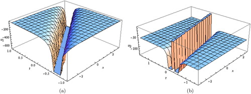
Figure 2. (a) Bright soliton solution for Equation (Equation17(17) $\begin{aligned} u_{3} (x, t) & = b_{1} (- \frac{ϵ (p + \sinh [\sqrt{β_{1}} (x - λ t + ζ_{0})])}{η \sqrt{p^{2} + 1} + \cosh [\sqrt{β_{1}} (x - λ t + ζ_{0})]} - 1) + (ϵ^{2} (η \sqrt{p^{2} + 1} \cosh [\sqrt{β_{1}} (x - λ t + ζ_{0})] + 1 \\ {- p \sinh [\sqrt{β_{1}} (x - λ t + ζ_{0})])}^{2} β_{1} d_{2})/ ({(η \sqrt{p^{2} + 1} + \cosh [\sqrt{β_{1}} (x - λ t + ζ_{0})])}^{2} \\ {(η \sqrt{p^{2} + 1} + p ϵ + \cosh [\sqrt{β_{1}} (x - λ t + ζ_{0})] + ϵ \sinh [\sqrt{β_{1}} (x - λ t + ζ_{0})])}^{2}) \\ - β_{2} d_{2} (- \frac{ϵ (p + \sinh [\sqrt{β_{1}} (x - λ t + ζ_{0})])}{η \sqrt{p^{2} + 1} + \cosh [\sqrt{β_{1}} (x - λ t + ζ_{0})]} - 1) \\ - β_{3} d_{2} {(\frac{ϵ (p + \sinh [\sqrt{β_{1}} (x - λ t + ζ_{0})])}{η \sqrt{p^{2} + 1} + \cosh [\sqrt{β_{1}} (x - λ t + ζ_{0})]} + 1)}^{2} \\ - \frac{\sqrt{b_{1}^{2} β_{2}^{2} κ^{2} + 4 β_{1} (β_{1} - b_{1}^{2} β_{3} κ^{2})} - b_{1} β_{2} κ + 2 β_{1} (β_{1} d_{2} κ + 1)}{2 β_{1} κ} . \end{aligned}$ (17) ), and (b) dark soliton solution for Equation (Equation19(19) $\begin{aligned} u_{4} (x, t) & = β_{1} d_{2} (ϵ \coth [\frac{1}{2} \sqrt{β_{1}} (x - λ t + ζ_{0})] + 1) + \frac{β_{1} d_{2} ϵ^{2} c s c h {[\frac{1}{2} \sqrt{β_{1}} (x - λ t + ζ_{0})]}^{4}}{4 {(ϵ \coth [\frac{1}{2} \sqrt{β_{1}} (x - λ t + ζ_{0})] + 1)}^{2}} \\ - \frac{b_{1} β_{1} (ϵ \coth [\frac{1}{2} \sqrt{β_{1}} (x - λ t + ζ_{0})] + 1)}{β_{2}} - \frac{β_{1}^{2} β_{3} d_{2} {(ϵ \coth [\frac{1}{2} \sqrt{β_{1}} (x - λ t + ζ_{0})] + 1)}^{2}}{β_{2}^{2}} \\ + \frac{\sqrt{b_{1}^{2} β_{2}^{2} κ^{2} + 4 β_{1} (β_{1} - b_{1}^{2} β_{3} κ^{2})} + b_{1} β_{2} κ - 2 β_{1} (β_{1} d_{2} κ + 1)}{2 β_{1} κ} . \end{aligned}$ (19) ).

Figure 2. (a) Bright soliton solution for Equation (Equation17(17) u3(x,t)=b1−ϵp+sinhβ1x−λt+ζ0ηp2+1+coshβ1x−λt+ζ0−1+ϵ2ηp2+1coshβ1x−λt+ζ0+1−psinhβ1x−λt+ζ02β1d2ηp2+1+coshβ1x−λt+ζ02ηp2+1+pϵ+coshβ1x−λt+ζ0+ϵsinhβ1x−λt+ζ02−β2d2−ϵp+sinhβ1x−λt+ζ0ηp2+1+coshβ1x−λt+ζ0−1−β3d2ϵp+sinhβ1x−λt+ζ0ηp2+1+coshβ1x−λt+ζ0+12−b12β22κ2+4β1β1−b12β3κ2−b1β2κ+2β1β1d2κ+12β1κ.(17) ), and (b) dark soliton solution for Equation (Equation19(19) u4(x,t)=β1d2ϵcoth12β1x−λt+ζ0+1+β1d2ϵ2csch12β1x−λt+ζ044ϵcoth12β1x−λt+ζ0+12−b1β1ϵcoth12β1x−λt+ζ0+1β2−β12β3d2ϵcoth12β1x−λt+ζ0+12β22+b12β22κ2+4β1β1−b12β3κ2+b1β2κ−2β1β1d2κ+12β1κ.(19) ).

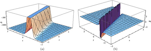
Figure 3. (a) Combined dark–bright soliton solutions for Equation (Equation20(20) $\begin{aligned} u_{5} (x, t) & = \frac{1}{4} (\frac{4 β_{1} d_{2} {(η ϵ \cosh [\sqrt{β_{1}} (x - λ t + ζ_{0})] + ϵ)}^{2}}{{(η + \cosh [\sqrt{β_{1}} (x - λ t + ζ_{0})])}^{2} {(η + \cosh [\sqrt{β_{1}} (x - λ t + ζ_{0})] + ϵ \sinh [\sqrt{β_{1}} (x - λ t + ζ_{0})])}^{2}} \\ β_{1} d_{2} (- {(\frac{ϵ \sinh [\sqrt{β_{1}} (x - λ t + ζ_{0})]}{η + \cosh [\sqrt{β_{1}} (x - λ t + ζ_{0})]} + 1)}^{2}) - 2 b_{1} \sqrt{\frac{β_{1}}{β_{3}}} (\frac{ϵ \sinh [\sqrt{β_{1}} (x - λ t + ζ_{0})]}{η + \cosh [\sqrt{β_{1}} (x - λ t + ζ_{0})]} + 1) \\ + 2 β_{2} \sqrt{\frac{β_{1}}{β_{3}}} d_{2} (\frac{ϵ \sinh [\sqrt{β_{1}} (x - λ t + ζ_{0})]}{η + \cosh [\sqrt{β_{1}} (x - λ t + ζ_{0})]} + 1) \\ + \frac{2 (\sqrt{β_{2}^{2} b_{1}^{2} κ^{2} - 4 β_{1} β_{3} b_{1}^{2} κ^{2} + 4 β_{1}^{2}} + b_{1} β_{2} κ - 2 β_{1} (β_{1} d_{2} κ + 1))}{β_{1} κ}) . \end{aligned}$ (20) ) and (b) bright soliton solutions for Equation (Equation21(21) $\begin{aligned} u_{6} (x, t) & = b_{1} (- \frac{ϵ (p + \sinh [\sqrt{β_{1}} (x - λ t + ζ_{0})])}{η \sqrt{p^{2} + 1} + \cosh [\sqrt{β_{1}} (x - λ t + ζ_{0})]} - 1) + (ϵ^{2} (η \sqrt{p^{2} + 1} \cosh [\sqrt{β_{1}} (x - λ t + ζ_{0})] + 1 \\ {- p \sinh [\sqrt{β_{1}} (x - λ t + ζ_{0})])}^{2} β_{1} d_{2})/ ({(η \sqrt{p^{2} + 1} + \cosh [\sqrt{β_{1}} (x - λ t + ζ_{0})])}^{2} \\ {(η \sqrt{p^{2} + 1} + p ϵ + \cosh [\sqrt{β_{1}} (x - λ t + ζ_{0})] + ϵ \sinh [\sqrt{β_{1}} (x - λ t + ζ_{0})])}^{2}) \\ - β_{2} d_{2} (- \frac{ϵ (p + \sinh [\sqrt{β_{1}} (x - λ t + ζ_{0})])}{η \sqrt{p^{2} + 1} + \cosh [\sqrt{β_{1}} (x - λ t + ζ_{0})]} - 1) \\ - β_{3} d_{2} {(\frac{ϵ (p + \sinh [\sqrt{β_{1}} (x - λ t + ζ_{0})])}{η \sqrt{p^{2} + 1} + \cosh [\sqrt{β_{1}} (x - λ t + ζ_{0})]} + 1)}^{2} \\ + \frac{\sqrt{b_{1}^{2} β_{2}^{2} κ^{2} + 4 β_{1} (β_{1} - b_{1}^{2} β_{3} κ^{2})} + b_{1} β_{2} κ - 2 β_{1} (β_{1} d_{2} κ + 1)}{2 β_{1} κ} . \end{aligned}$ (21) ).

Figure 3. (a) Combined dark–bright soliton solutions for Equation (Equation20(20) u5x,t=144β1d2ηϵcoshβ1x−λt+ζ0+ϵ2η+coshβ1x−λt+ζ02η+coshβ1x−λt+ζ0+ϵsinhβ1x−λt+ζ02β1d2−ϵsinhβ1x−λt+ζ0η+coshβ1x−λt+ζ0+12−2b1β1β3ϵsinhβ1x−λt+ζ0η+coshβ1x−λt+ζ0+1+2β2β1β3d2ϵsinhβ1x−λt+ζ0η+coshβ1x−λt+ζ0+1+2β22b12κ2−4β1β3b12κ2+4β12+b1β2κ−2β1β1d2κ+1β1κ.(20) ) and (b) bright soliton solutions for Equation (Equation21(21) u6(x,t)=b1−ϵp+sinhβ1x−λt+ζ0ηp2+1+coshβ1x−λt+ζ0−1+ϵ2ηp2+1coshβ1x−λt+ζ0+1−psinhβ1x−λt+ζ02β1d2ηp2+1+coshβ1x−λt+ζ02ηp2+1+pϵ+coshβ1x−λt+ζ0+ϵsinhβ1x−λt+ζ02−β2d2−ϵp+sinhβ1x−λt+ζ0ηp2+1+coshβ1x−λt+ζ0−1−β3d2ϵp+sinhβ1x−λt+ζ0ηp2+1+coshβ1x−λt+ζ0+12+b12β22κ2+4β1β1−b12β3κ2+b1β2κ−2β1β1d2κ+12β1κ.(21) ).

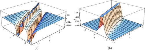
Figure 4. (a) Dark soliton solution for Equation (Equation23(23) $\begin{aligned} u_{7} (x, t) & = \frac{β_{1} d_{2} ϵ^{2} c s c h {[\frac{1}{2} \sqrt{β_{1}} (x - λ t + ζ_{0})]}^{4}}{4 {(ϵ \coth [\frac{1}{2} \sqrt{β_{1}} (x - λ t + ζ_{0})] + 1)}^{2}} + β_{1} d_{2} (ϵ \coth [\frac{1}{2} \sqrt{β_{1}} (x - λ t + ζ_{0})] + 1) \\ - \frac{2 β_{1} (A - 2 β_{1} β_{2} κ (ε + κ)) (ϵ \coth [\frac{1}{2} \sqrt{β_{1}} (x - λ t + ζ_{0})] + 1)}{β_{2} κ (β_{2}^{2} (ε^{2} - 4 κ^{2}) - 4 β_{1} β_{3} ε^{2})} \\ - \frac{β_{3} β_{1}^{2} d_{2} {(ϵ \coth [\frac{1}{2} \sqrt{β_{1}} (x - λ t + ζ_{0})] + 1)}^{2}}{β_{2}^{2}} \\ + \frac{- A β_{2} (ε - 2 κ) - 4 β_{3} β_{1}^{2} ε^{2} κ (β_{1} d_{2} ε - 1) + β_{2}^{2} β_{1} ε κ (ε - 2 κ) (β_{1} d_{2} (ε + 2 κ) + 1)}{β_{1} ε κ (4 β_{1} β_{3} ε^{2} - β_{2}^{2} (ε^{2} - 4 κ^{2}))} . \end{aligned}$ (23) ) and (b) Kink wave soliton solution for Equation (Equation24(24) $\begin{aligned} u_{8} (x, t) & = \frac{β_{1} d_{2} {(η ϵ \cosh [\sqrt{β_{1}} (x - λ t + ζ_{0})] + ϵ)}^{2}}{{(η + \cosh [\sqrt{β_{1}} (x - λ t + ζ_{0})])}^{2} {(η + \cosh [\sqrt{β_{1}} (x - λ t + ζ_{0})] + ϵ \sinh [\sqrt{β_{1}} (x - λ t + ζ_{0})])}^{2}} \\ - \frac{1}{4} β_{1} d_{2} {(\frac{ϵ \sinh [\sqrt{β_{1}} (x - λ t + ζ_{0})]}{η + \cosh [\sqrt{β_{1}} (x - λ t + ζ_{0})]} + 1)}^{2} + \frac{1}{2} β_{2} \sqrt{\frac{β_{1}}{β_{3}}} d_{2} (\frac{ϵ \sinh [\sqrt{β_{1}} (x - λ t + ζ_{0})]}{η + \cosh [\sqrt{β_{1}} (x - λ t + ζ_{0})]} + 1) \\ - \frac{\sqrt{\frac{β_{1}}{β_{3}}} (A - 2 β_{1} β_{2} κ (ε + κ)) (\frac{ϵ \sinh [\sqrt{β_{1}} (x - λ t + ζ_{0})]}{η + \cosh [\sqrt{β_{1}} (x - λ t + ζ_{0})]} + 1)}{κ (β_{2}^{2} (ε^{2} - 4 κ^{2}) - 4 β_{1} β_{3} ε^{2})} \\ + \frac{- A β_{2} (ε - 2 κ) - 4 β_{3} β_{1}^{2} ε^{2} κ (β_{1} d_{2} ε - 1) + β_{2}^{2} β_{1} ε κ (ε - 2 κ) (β_{1} d_{2} (ε + 2 κ) + 1)}{β_{1} ε κ (4 β_{1} β_{3} ε^{2} - β_{2}^{2} (ε^{2} - 4 κ^{2}))} . \end{aligned}$ (24) ).

Figure 4. (a) Dark soliton solution for Equation (Equation23(23) u7(x,t)=β1d2ϵ2csch12β1x−λt+ζ044ϵcoth12β1x−λt+ζ0+12+β1d2ϵcoth12β1x−λt+ζ0+1−2β1A−2β1β2κ(ε+κ)ϵcoth12β1x−λt+ζ0+1β2κβ22ε2−4κ2−4β1β3ε2−β3β12d2ϵcoth12β1x−λt+ζ0+12β22+−Aβ2(ε−2κ)−4β3β12ε2κβ1d2ε−1+β22β1εκ(ε−2κ)β1d2(ε+2κ)+1β1εκ4β1β3ε2−β22ε2−4κ2.(23) ) and (b) Kink wave soliton solution for Equation (Equation24(24) u8(x,t)=β1d2ηϵcoshβ1x−λt+ζ0+ϵ2η+coshβ1x−λt+ζ02η+coshβ1x−λt+ζ0+ϵsinhβ1x−λt+ζ02−14β1d2ϵsinhβ1x−λt+ζ0η+coshβ1x−λt+ζ0+12+12β2β1β3d2ϵsinhβ1x−λt+ζ0η+coshβ1x−λt+ζ0+1−β1β3A−2β1β2κ(ε+κ)ϵsinhβ1x−λt+ζ0η+coshβ1x−λt+ζ0+1κβ22ε2−4κ2−4β1β3ε2+−Aβ2(ε−2κ)−4β3β12ε2κβ1d2ε−1+β22β1εκ(ε−2κ)β1d2(ε+2κ)+1β1εκ4β1β3ε2−β22ε2−4κ2.(24) ).

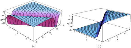
Figure 5. (a,b) Solitary wave solutions for Equation (Equation25(25) $\begin{aligned} u_{9} (x, t) & = β_{1} d_{2} ϵ^{2} {(η \sqrt{p^{2} + 1} \cosh [\sqrt{β_{1}} (x - λ t + ζ_{0})] - p \sinh [\sqrt{β_{1}} (x - λ t + ζ_{0})] + 1)}^{2}/ \\ ({(η \sqrt{p^{2} + 1} + \cosh [\sqrt{β_{1}} (x - λ t + ζ_{0})])}^{2} \\ {(η \sqrt{p^{2} + 1} + p ϵ + \cosh [\sqrt{β_{1}} (x - λ t + ζ_{0})] + ϵ \sinh [\sqrt{β_{1}} (x - λ t + ζ_{0})])}^{2}) \\ - β_{2} d_{2} (- \frac{ϵ (p + \sinh [\sqrt{β_{1}} (x - λ t + ζ_{0})])}{η \sqrt{p^{2} + 1} + \cosh [\sqrt{β_{1}} (x - λ t + ζ_{0})]} - 1) \\ - β_{3} d_{2} {(\frac{ϵ (p + \sinh [\sqrt{β_{1}} (x - λ t + ζ_{0})])}{η \sqrt{p^{2} + 1} + \cosh [\sqrt{β_{1}} (x - λ t + ζ_{0})]} + 1)}^{2} \\ + \frac{2 (A - 2 β_{1} β_{2} κ (ε + κ)) (- \frac{ϵ (p + \sinh [\sqrt{β_{1}} (x - λ t + ζ_{0})])}{η \sqrt{p^{2} + 1} + \cosh [\sqrt{β_{1}} (x - λ t + ζ_{0})]} - 1)}{κ (β_{2}^{2} (ε^{2} - 4 κ^{2}) - 4 β_{1} β_{3} ε^{2})} \\ + \frac{- A β_{2} (ε - 2 κ) - 4 β_{3} β_{1}^{2} ε^{2} κ (β_{1} d_{2} ε - 1) + β_{2}^{2} β_{1} ε κ (ε - 2 κ) (β_{1} d_{2} (ε + 2 κ) + 1)}{β_{1} ε κ (β_{2}^{2} (4 κ^{2} - ε^{2}) + 4 β_{1} β_{3} ε^{2})} . \end{aligned}$ (25) ) and Equation (Equation27(27) $\begin{aligned} u_{10} (x, t) & = \frac{1}{4} β_{1} d_{2} ϵ (4 \coth [\frac{1}{2} \sqrt{β_{1}} (x - λ t + ζ_{0})] + \frac{ϵ c s c h {[\frac{1}{2} \sqrt{β_{1}} (x - λ t + ζ_{0})]}^{4}}{{(ϵ \coth [\frac{1}{2} \sqrt{β_{1}} (x - λ t + ζ_{0})] + 1)}^{2}}) \\ + \frac{β_{2} (\sqrt{b_{1}^{2} β_{2}^{2} κ^{2} + 4 β_{1}^{2}} - 2 β_{1}) + b_{1} κ (β_{2}^{2} - 2 β_{1}^{2} (ϵ \coth [\frac{1}{2} \sqrt{β_{1}} (x - λ t + ζ_{0})] + 1))}{2 β_{1} β_{2} κ} . \end{aligned}$ (27) ).

Figure 5. (a,b) Solitary wave solutions for Equation (Equation25(25) u9(x,t)=β1d2ϵ2ηp2+1coshβ1x−λt+ζ0−psinhβ1x−λt+ζ0+12ηp2+1+coshβ1x−λt+ζ02ηp2+1+pϵ+coshβ1x−λt+ζ0+ϵsinhβ1x−λt+ζ02−β2d2−ϵp+sinhβ1x−λt+ζ0ηp2+1+coshβ1x−λt+ζ0−1−β3d2ϵp+sinhβ1x−λt+ζ0ηp2+1+coshβ1x−λt+ζ0+12+2A−2β1β2κ(ε+κ)−ϵp+sinhβ1x−λt+ζ0ηp2+1+coshβ1x−λt+ζ0−1κβ22ε2−4κ2−4β1β3ε2+−Aβ2(ε−2κ)−4β3β12ε2κβ1d2ε−1+β22β1εκ(ε−2κ)β1d2(ε+2κ)+1β1εκβ224κ2−ε2+4β1β3ε2.(25) ) and Equation (Equation27(27) u10(x,t)=14β1d2ϵ4coth12β1x−λt+ζ0+ϵcsch12β1x−λt+ζ04ϵcoth12β1x−λt+ζ0+12+β2b12β22κ2+4β12−2β1+b1κβ22−2β12ϵcoth12β1x−λt+ζ0+12β1β2κ.(27) ).

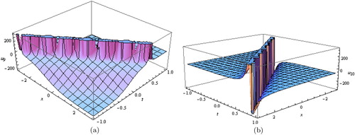
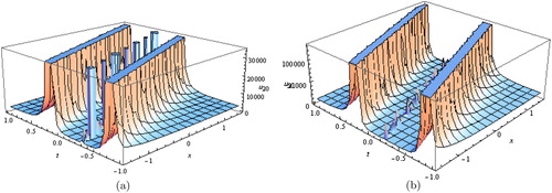
Figure 6. (a,b) Solitary traveling wave solutions for Equation (Equation28(28) $\begin{aligned} u_{11} (x, t) & = \frac{1}{2} (\frac{2 β_{1} d_{2} {(η ϵ \cosh [\sqrt{β_{1}} (x - λ t + ζ_{0})] + ϵ)}^{2}}{{(η + \cosh [\sqrt{β_{1}} (x - λ t + ζ_{0})])}^{2} {(η + \cosh [\sqrt{β_{1}} (x - λ t + ζ_{0})] + ϵ \sinh [\sqrt{β_{1}} (x - λ t + ζ_{0})])}^{2}} \\ + \frac{\sqrt{b_{1}^{2} β_{2}^{2} κ^{2} + 4 β_{1}^{2}} + b_{1} β_{2} κ - 2 β_{1} (β_{1} d_{2} κ + 1)}{β_{1} κ} - b_{1} \sqrt{\frac{β_{1}}{β_{3}}} (\frac{ϵ \sinh [\sqrt{β_{1}} (x - λ t + ζ_{0})]}{η + \cosh [\sqrt{β_{1}} (x - λ t + ζ_{0})]} + 1) \\ + (\frac{ϵ \sinh [\sqrt{β_{1}} (x - λ t + ζ_{0})]}{η + \cosh [\sqrt{β_{1}} (x - λ t + ζ_{0})]} + 1) β_{2} \sqrt{\frac{β_{1}}{β_{3}}} d_{2}) . \end{aligned}$ (28) ) and Equation (Equation29(29) $\begin{aligned} u_{12} (x, t) & = b_{1} (- \frac{ϵ (p + \sinh [\sqrt{β_{1}} (x - λ t + ζ_{0})])}{η \sqrt{p^{2} + 1} + \cosh [\sqrt{β_{1}} (x - λ t + ζ_{0})]} - 1) + (ϵ^{2} (η \sqrt{p^{2} + 1} \cosh [\sqrt{β_{1}} (x - λ t + ζ_{0})] + 1 \\ {- p \sinh [\sqrt{β_{1}} (x - λ t + ζ_{0})])}^{2} β_{1} d_{2})/ ({(η \sqrt{p^{2} + 1} + \cosh [\sqrt{β_{1}} (x - λ t + ζ_{0})])}^{2} \\ {(η \sqrt{p^{2} + 1} + p ϵ + \cosh [\sqrt{β_{1}} (x - λ t + ζ_{0})] + ϵ \sinh [\sqrt{β_{1}} (x - λ t + ζ_{0})])}^{2}) \\ - \frac{\sqrt{b_{1}^{2} β_{2}^{2} κ^{2} + 4 β_{1}^{2}} + b_{1} β_{2} κ - 2 β_{1} (β_{1} d_{2} κ + 1)}{2 β_{1} κ} + β_{2} d_{2} (- \frac{ϵ (p + \sinh [\sqrt{β_{1}} (x - λ t + ζ_{0})])}{η \sqrt{p^{2} + 1} + \cosh [\sqrt{β_{1}} (x - λ t + ζ_{0})]} - 1) . \end{aligned}$ (29) ).

Figure 6. (a,b) Solitary traveling wave solutions for Equation (Equation28(28) u11(x,t)=122β1d2ηϵcoshβ1x−λt+ζ0+ϵ2η+coshβ1x−λt+ζ02η+coshβ1x−λt+ζ0+ϵsinhβ1x−λt+ζ02+b12β22κ2+4β12+b1β2κ−2β1β1d2κ+1β1κ−b1β1β3ϵsinhβ1x−λt+ζ0η+coshβ1x−λt+ζ0+1+ϵsinhβ1x−λt+ζ0η+coshβ1x−λt+ζ0+1β2β1β3d2.(28) ) and Equation (Equation29(29) u12(x,t)=b1−ϵp+sinhβ1x−λt+ζ0ηp2+1+coshβ1x−λt+ζ0−1+ϵ2ηp2+1coshβ1x−λt+ζ0+1−psinhβ1x−λt+ζ02β1d2ηp2+1+coshβ1x−λt+ζ02ηp2+1+pϵ+coshβ1x−λt+ζ0+ϵsinhβ1x−λt+ζ02−b12β22κ2+4β12+b1β2κ−2β1β1d2κ+12β1κ+β2d2−ϵp+sinhβ1x−λt+ζ0ηp2+1+coshβ1x−λt+ζ0−1.(29) ).

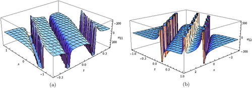
Figure 7. (a) Solitary wave solution for Equation (Equation31(31) $\begin{aligned} u_{13} (x, t) & = β_{1} d_{2} (ϵ \coth [\frac{1}{2} \sqrt{β_{1}} (x - λ t + ζ_{0})] + 1) + \frac{β_{1} d_{2} ϵ^{2} c s c h {[\frac{1}{2} \sqrt{β_{1}} (x - λ t + ζ_{0})]}^{4}}{4 {(ϵ \coth [\frac{1}{2} \sqrt{β_{1}} (x - λ t + ζ_{0})] + 1)}^{2}} \\ - \frac{2 β_{1} (\sqrt{β_{1}^{2} β_{2}^{2} ε^{2} κ (2 ε + 5 κ)} + 2 β_{1} β_{2} κ (ε + κ)) (ϵ \coth [\frac{1}{2} \sqrt{β_{1}} (x - λ t + ζ_{0})] + 1)}{β_{2}^{3} (4 κ^{3} - ε^{2} κ)} \\ - \frac{\sqrt{β_{1}^{2} β_{2}^{2} ε^{2} κ (2 ε + 5 κ)} + β_{1} β_{2} ε κ (β_{1} d_{2} (ε + 2 κ) + 1)}{β_{1} β_{2} ε κ (ε + 2 κ)} . \end{aligned}$ (31) ) and (b) solitary traveling wave solution for Equation (Equation32(32) $\begin{aligned} u_{14} (x, t) & = \frac{β_{1} d_{2} {(η ϵ \cosh [\sqrt{β_{1}} (x - λ t + ζ_{0})] + ϵ)}^{2}}{{(η + \cosh [\sqrt{β_{1}} (x - λ t + ζ_{0})])}^{2} {(η + \cosh [\sqrt{β_{1}} (x - λ t + ζ_{0})] + ϵ \sinh [\sqrt{β_{1}} (x - λ t + ζ_{0})])}^{2}} \\ - \frac{\sqrt{β_{1}^{2} β_{2}^{2} ε^{2} κ (2 ε + 5 κ)} + β_{1} β_{2} ε κ (β_{1} d_{2} (ε + 2 κ) + 1)}{β_{1} β_{2} ε κ (ε + 2 κ)} \\ + \frac{1}{2} β_{2} \sqrt{\frac{β_{1}}{β_{3}}} d_{2} (\frac{ϵ \sinh [\sqrt{β_{1}} (x - λ t + ζ_{0})]}{η + \cosh [\sqrt{β_{1}} (x - λ t + ζ_{0})]} + 1) \\ - \frac{\sqrt{\frac{β_{1}}{β_{3}}} (\sqrt{β_{1}^{2} β_{2}^{2} ε^{2} κ (2 ε + 5 κ)} + 2 β_{1} β_{2} κ (ε + κ)) (\frac{ϵ \sinh [\sqrt{β_{1}} (x - λ t + ζ_{0})]}{η + \cosh [\sqrt{β_{1}} (x - λ t + ζ_{0})]} + 1)}{β_{2}^{2} (4 κ^{3} - ε^{2} κ)} . \end{aligned}$ (32) ).

Figure 7. (a) Solitary wave solution for Equation (Equation31(31) u13(x,t)=β1d2ϵcoth12β1x−λt+ζ0+1+β1d2ϵ2csch12β1x−λt+ζ044ϵcoth12β1x−λt+ζ0+12−2β1β12β22ε2κ(2ε+5κ)+2β1β2κ(ε+κ)ϵcoth12β1x−λt+ζ0+1β234κ3−ε2κ−β12β22ε2κ(2ε+5κ)+β1β2εκβ1d2(ε+2κ)+1β1β2εκ(ε+2κ).(31) ) and (b) solitary traveling wave solution for Equation (Equation32(32) u14(x,t)=β1d2ηϵcoshβ1x−λt+ζ0+ϵ2η+coshβ1x−λt+ζ02η+coshβ1x−λt+ζ0+ϵsinhβ1x−λt+ζ02−β12β22ε2κ(2ε+5κ)+β1β2εκβ1d2(ε+2κ)+1β1β2εκ(ε+2κ)+12β2β1β3d2ϵsinhβ1x−λt+ζ0η+coshβ1x−λt+ζ0+1−β1β3β12β22ε2κ(2ε+5κ)+2β1β2κ(ε+κ)ϵsinhβ1x−λt+ζ0η+coshβ1x−λt+ζ0+1β224κ3−ε2κ.(32) ).

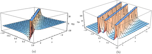
Figure 8. (a) Solitary traveling wave solution for Equation (Equation33(33) $\begin{aligned} u_{15} (x, t) & = β_{1} d_{2} ϵ^{2} {(η \sqrt{p^{2} + 1} \cosh [\sqrt{β_{1}} (x - λ t + ζ_{0})] - p \sinh [\sqrt{β_{1}} (x - λ t + ζ_{0})] + 1)}^{2}/ \\ ({(η \sqrt{p^{2} + 1} + \cosh [\sqrt{β_{1}} (x - λ t + ζ_{0})])}^{2} (η \sqrt{p^{2} + 1} + p ϵ + \cosh [\sqrt{β_{1}} (x - λ t + ζ_{0})] \\ {+ ϵ \sinh [\sqrt{β_{1}} (x - λ t + ζ_{0})])}^{2}) β_{2} d_{2} (- (- \frac{ϵ (p + \sinh [\sqrt{β_{1}} (x - λ t + ζ_{0})])}{η \sqrt{p^{2} + 1} + \cosh [\sqrt{β_{1}} (x - λ t + ζ_{0})]} - 1)) \\ + \frac{2 (\sqrt{β_{1}^{2} β_{2}^{2} ε^{2} κ (2 ε + 5 κ)} + 2 β_{1} β_{2} κ (ε + κ)) (- \frac{ϵ (p + \sinh [\sqrt{β_{1}} (x - λ t + ζ_{0})])}{η \sqrt{p^{2} + 1} + \cosh [\sqrt{β_{1}} (x - λ t + ζ_{0})]} - 1)}{β_{2}^{2} (4 κ^{3} - ε^{2} κ)} \\ - \frac{\sqrt{β_{1}^{2} β_{2}^{2} ε^{2} κ (2 ε + 5 κ)} + β_{1} β_{2} ε κ (β_{1} d_{2} (ε + 2 κ) + 1)}{β_{1} β_{2} ε κ (ε + 2 κ)} . \end{aligned}$ (33) ) and (b) bright soliton solution for Equation (Equation36(36) $\begin{aligned} u_{17} (x, t) & = a_{0} + \frac{β_{1} d_{2} {(η ϵ \cosh [\sqrt{β_{1}} (x - λ t + ζ_{0})] + ϵ)}^{2}}{{(η + \cosh [\sqrt{β_{1}} (x - λ t + ζ_{0})])}^{2} {(η + \cosh [\sqrt{β_{1}} (x - λ t + ζ_{0})] + ϵ \sinh [\sqrt{β_{1}} (x - λ t + ζ_{0})])}^{2}} \\ - \frac{1}{4} β_{1} d_{2} {(\frac{ϵ \sinh [\sqrt{β_{1}} (x - λ t + ζ_{0})]}{η + \cosh [\sqrt{β_{1}} (x - λ t + ζ_{0})]} + 1)}^{2} + \frac{1}{2} β_{2} \sqrt{\frac{β_{1}}{β_{3}}} d_{2} (\frac{ϵ \sinh [\sqrt{β_{1}} (x - λ t + ζ_{0})]}{η + \cosh [\sqrt{β_{1}} (x - λ t + ζ_{0})]} + 1) . \end{aligned}$ (36) ).

Figure 8. (a) Solitary traveling wave solution for Equation (Equation33(33) u15(x,t)=β1d2ϵ2ηp2+1coshβ1x−λt+ζ0−psinhβ1x−λt+ζ0+12ηp2+1+coshβ1x−λt+ζ02ηp2+1+pϵ+coshβ1x−λt+ζ0+ϵsinhβ1x−λt+ζ02)β2d2−−ϵp+sinhβ1x−λt+ζ0ηp2+1+coshβ1x−λt+ζ0−1+2β12β22ε2κ(2ε+5κ)+2β1β2κ(ε+κ)−ϵp+sinhβ1x−λt+ζ0ηp2+1+coshβ1x−λt+ζ0−1β224κ3−ε2κ−β12β22ε2κ(2ε+5κ)+β1β2εκβ1d2(ε+2κ)+1β1β2εκ(ε+2κ).(33) ) and (b) bright soliton solution for Equation (Equation36(36) u17(x,t)=a0+β1d2ηϵcoshβ1x−λt+ζ0+ϵ2η+coshβ1x−λt+ζ02η+coshβ1x−λt+ζ0+ϵsinhβ1x−λt+ζ02−14β1d2ϵsinhβ1x−λt+ζ0η+coshβ1x−λt+ζ0+12+12β2β1β3d2ϵsinhβ1x−λt+ζ0η+coshβ1x−λt+ζ0+1.(36) ).

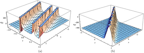
Figure 9. (a) Solitary wave solutions for Equation (Equation37(37) $\begin{aligned} u_{18} (x, t) & = a_{0} + β_{1} d_{2} ϵ^{2} {(η \sqrt{p^{2} + 1} \cosh [\sqrt{β_{1}} (x - λ t + ζ_{0})] - p \sinh [\sqrt{β_{1}} (x - λ t + ζ_{0})] + 1)}^{2}/ \\ ({(η \sqrt{p^{2} + 1} + \cosh [\sqrt{β_{1}} (x - λ t + ζ_{0})])}^{2} \\ {(η \sqrt{p^{2} + 1} + p ϵ + \cosh [\sqrt{β_{1}} (x - λ t + ζ_{0})] + ϵ \sinh [\sqrt{β_{1}} (x - λ t + ζ_{0})])}^{2}) \\ - β_{2} d_{2} (- \frac{ϵ (p + \sinh [\sqrt{β_{1}} (x - λ t + ζ_{0})])}{η \sqrt{p^{2} + 1} + \cosh [\sqrt{β_{1}} (x - λ t + ζ_{0})]} - 1) \\ - β_{3} d_{2} {(\frac{ϵ (p + \sinh [\sqrt{β_{1}} (x - λ t + ζ_{0})])}{η \sqrt{p^{2} + 1} + \cosh [\sqrt{β_{1}} (x - λ t + ζ_{0})]} + 1)}^{2} . \end{aligned}$ (37) ) and (b) bright soliton solution for Equation (Equation39(39) $\begin{aligned} u_{19} (x, t) & = \frac{1}{4} (\frac{2}{ε} + \frac{2}{κ} - \frac{3}{ε + κ} - 4 β_{1} d_{2} + 4 β_{1} d_{2} (ϵ \coth [\frac{1}{2} \sqrt{β_{1}} (x - λ t + ζ_{0})] + 1) \\ - \frac{β_{1} d_{2} (ε^{2} - 4 κ^{2}) {(ϵ \coth [\frac{1}{2} \sqrt{β_{1}} (x - λ t + ζ_{0})] + 1)}^{2}}{ε^{2}} \\ + \frac{β_{1} d_{2} ϵ^{2} c s c h {[\frac{1}{2} \sqrt{β_{1}} (x - λ t + ζ_{0})]}^{4}}{{(ϵ \coth [\frac{1}{2} \sqrt{β_{1}} (x - λ t + ζ_{0})] + 1)}^{2}} - \frac{2 β_{1}^{2} (2 ε + κ) (ϵ \coth [\frac{1}{2} \sqrt{β_{1}} (x - λ t + ζ_{0})] + 1)}{β_{2}^{2} κ (ε + κ)}) . \end{aligned}$ (39) ).

Figure 9. (a) Solitary wave solutions for Equation (Equation37(37) u18(x,t)=a0+β1d2ϵ2ηp2+1coshβ1x−λt+ζ0−psinhβ1x−λt+ζ0+12ηp2+1+coshβ1x−λt+ζ02ηp2+1+pϵ+coshβ1x−λt+ζ0+ϵsinhβ1x−λt+ζ02−β2d2−ϵp+sinhβ1x−λt+ζ0ηp2+1+coshβ1x−λt+ζ0−1−β3d2ϵp+sinhβ1x−λt+ζ0ηp2+1+coshβ1x−λt+ζ0+12.(37) ) and (b) bright soliton solution for Equation (Equation39(39) u19(x,t)=142ε+2κ−3ε+κ−4β1d2+4β1d2ϵcoth12β1x−λt+ζ0+1−β1d2ε2−4κ2ϵcoth12β1x−λt+ζ0+12ε2+β1d2ϵ2csch12β1x−λt+ζ04ϵcoth12β1x−λt+ζ0+12−2β12(2ε+κ)ϵcoth12β1x−λt+ζ0+1β22κ(ε+κ).(39) ).

Figure 10. (a,b) Solitary wave solutions for Equation (Equation40(40) $\begin{aligned} u_{20} (x, t) & = \frac{1}{16} (\frac{16 β_{1} d_{2} {(η ϵ \cosh [\sqrt{β_{1}} (x - λ t + ζ_{0})] + ϵ)}^{2}}{{(η + \cosh [\sqrt{β_{1}} (x - λ t + ζ_{0})])}^{2} {(η + \cosh [\sqrt{β_{1}} (x - λ t + ζ_{0})] + ϵ \sinh [\sqrt{β_{1}} (x - λ t + ζ_{0})])}^{2}} \\ + 4 (- 4 β_{1} d_{2} - \frac{3}{ε + κ} + \frac{2}{ε} + \frac{2}{κ}) - \frac{4 β_{1} \sqrt{\frac{β_{1}}{β_{3}}} (2 ε + κ) (\frac{ϵ \sinh [\sqrt{β_{1}} (x - λ t + ζ_{0})]}{η + \cosh [\sqrt{β_{1}} (x - λ t + ζ_{0})]} + 1)}{β_{2} κ (ε + κ)} \\ + 8 β_{2} \sqrt{\frac{β_{1}}{β_{3}}} d_{2} (\frac{ϵ \sinh [\sqrt{β_{1}} (x - λ t + ζ_{0})]}{η + \cosh [\sqrt{β_{1}} (x - λ t + ζ_{0})]} + 1) - \frac{β_{2}^{2} d_{2} (ε^{2} - 4 κ^{2}) {(\frac{ϵ \sinh [\sqrt{β_{1}} (x - λ t + ζ_{0})]}{η + \cosh [\sqrt{β_{1}} (x - λ t + ζ_{0})]} + 1)}^{2}}{β_{3} ε^{2}}) . \end{aligned}$ (40) ) and Equation (Equation41(41) $\begin{aligned} u_{21} (x, t) & = \frac{1}{4} (\frac{2}{ε} + \frac{2}{κ} - \frac{3}{ε + κ} - 4 β_{1} d_{2} + (4 ϵ^{2} (η \sqrt{p^{2} + 1} \cosh [\sqrt{β_{1}} (x - λ t + ζ_{0})] + 1 \\ {- p \sinh [\sqrt{β_{1}} (x - λ t + ζ_{0})])}^{2} β_{1} d_{2})/ ({(η \sqrt{p^{2} + 1} + \cosh [\sqrt{β_{1}} (x - λ t + ζ_{0})])}^{2} \\ {(η \sqrt{p^{2} + 1} + p ϵ + \cosh [\sqrt{β_{1}} (x - λ t + ζ_{0})] + ϵ \sinh [\sqrt{β_{1}} (x - λ t + ζ_{0})])}^{2}) \\ + \frac{2 β_{1} (2 ε + κ) (- \frac{ϵ (p + \sinh [\sqrt{β_{1}} (x - λ t + ζ_{0})])}{η \sqrt{p^{2} + 1} + \cosh [\sqrt{β_{1}} (x - λ t + ζ_{0})]} - 1)}{β_{2} κ (ε + κ)} - 4 (- \frac{ϵ (p + \sinh [\sqrt{β_{1}} (x - λ t + ζ_{0})])}{η \sqrt{p^{2} + 1} + \cosh [\sqrt{β_{1}} (x - λ t + ζ_{0})]} - 1) \\ β_{2} d_{2} - \frac{β_{2}^{2} d_{2} (ε^{2} - 4 κ^{2}) {(\frac{ϵ (p + \sinh [\sqrt{β_{1}} (x - λ t + ζ_{0})])}{η \sqrt{p^{2} + 1} + \cosh [\sqrt{β_{1}} (x - λ t + ζ_{0})]} + 1)}^{2}}{β_{1} ε^{2}}) . \end{aligned}$ (41) ).

Figure 10. (a,b) Solitary wave solutions for Equation (Equation40(40) u20(x,t)=11616β1d2ηϵcoshβ1x−λt+ζ0+ϵ2η+coshβ1x−λt+ζ02η+coshβ1x−λt+ζ0+ϵsinhβ1x−λt+ζ02+4−4β1d2−3ε+κ+2ε+2κ−4β1β1β3(2ε+κ)ϵsinhβ1x−λt+ζ0η+coshβ1x−λt+ζ0+1β2κ(ε+κ)+8β2β1β3d2ϵsinhβ1x−λt+ζ0η+coshβ1x−λt+ζ0+1−β22d2ε2−4κ2ϵsinhβ1x−λt+ζ0η+coshβ1x−λt+ζ0+12β3ε2.(40) ) and Equation (Equation41(41) u21(x,t)=142ε+2κ−3ε+κ−4β1d2+4ϵ2ηp2+1coshβ1x−λt+ζ0+1−psinhβ1x−λt+ζ02β1d2ηp2+1+coshβ1x−λt+ζ02ηp2+1+pϵ+coshβ1x−λt+ζ0+ϵsinhβ1x−λt+ζ02+2β1(2ε+κ)−ϵp+sinhβ1x−λt+ζ0ηp2+1+coshβ1x−λt+ζ0−1β2κ(ε+κ)−4−ϵp+sinhβ1x−λt+ζ0ηp2+1+coshβ1x−λt+ζ0−1β2d2−β22d2ε2−4κ2ϵp+sinhβ1x−λt+ζ0ηp2+1+coshβ1x−λt+ζ0+12β1ε2.(41) ).

In Figure (a), dark soliton solution for Equation (Equation15(15) $\begin{aligned} u_{1} (x, t) & = β_{1} d_{2} (ϵ \coth [\frac{1}{2} \sqrt{β_{1}} (x - λ t + ζ_{0})] + 1) + \frac{β_{1} d_{2} ϵ^{2} c s c h {[\frac{1}{2} \sqrt{β_{1}} (x - λ t + ζ_{0})]}^{4}}{4 {(ϵ \coth [\frac{1}{2} \sqrt{β_{1}} (x - λ t + ζ_{0})] + 1)}^{2}} \\ - \frac{b_{1} β_{1} (ϵ \coth [\frac{1}{2} \sqrt{β_{1}} (x - λ t + ζ_{0})] + 1)}{β_{2}} - \frac{β_{1}^{2} β_{3} d_{2} {(ϵ \coth [\frac{1}{2} \sqrt{β_{1}} (x - λ t + ζ_{0})] + 1)}^{2}}{β_{2}^{2}} \\ - \frac{\sqrt{b_{1}^{2} β_{2}^{2} κ^{2} + 4 β_{1} (β_{1} - b_{1}^{2} β_{3} κ^{2})} - b_{1} β_{2} κ + 2 β_{1} (β_{1} d_{2} κ + 1)}{2 β_{1} κ} . \end{aligned}$ (15) ) and (b) bright soliton solution for Equation (Equation16(16) $\begin{aligned} u_{2} (x, t) & = \frac{1}{4} (\frac{4 β_{1} d_{2} {(η ϵ \cosh [\sqrt{β_{1}} (x - λ t + ζ_{0})] + ϵ)}^{2}}{{(η + \cosh [\sqrt{β_{1}} (x - λ t + ζ_{0})])}^{2} {(η + \cosh [\sqrt{β_{1}} (x - λ t + ζ_{0})] + ϵ \sinh [\sqrt{β_{1}} (x - λ t + ζ_{0})])}^{2}} \\ - 2 b_{1} \sqrt{\frac{β_{1}}{β_{3}}} (\frac{ϵ \sinh [\sqrt{β_{1}} (x - λ t + ζ_{0})]}{η + \cosh [\sqrt{β_{1}} (x - λ t + ζ_{0})]} + 1) - β_{1} d_{2} {(\frac{ϵ \sinh [\sqrt{β_{1}} (x - λ t + ζ_{0})]}{η + \cosh [\sqrt{β_{1}} (x - λ t + ζ_{0})]} + 1)}^{2} \\ + 2 β_{2} \sqrt{\frac{β_{1}}{β_{3}}} d_{2} (\frac{ϵ \sinh [\sqrt{β_{1}} (x - λ t + ζ_{0})]}{η + \cosh [\sqrt{β_{1}} (x - λ t + ζ_{0})]} + 1) \\ - \frac{2 (\sqrt{β_{2}^{2} b_{1}^{2} κ^{2} - 4 β_{1} β_{3} b_{1}^{2} κ^{2} + 4 β_{1}^{2}} - b_{1} β_{2} κ + 2 β_{1} (β_{1} d_{2} κ + 1))}{β_{1} κ}) . \end{aligned}$ (16) ), with these parameters values $β_{1} = 2, β_{2} = 4, β_{3} = 2, ϵ = 8, η = 2, ζ_{0} = 0.3, λ = 4, κ = 0.4, b_{1} = 1.5, d_{2} = 2$ . In Figure , 3D (a) bright soliton solution for Equation (Equation17(17) $\begin{aligned} u_{3} (x, t) & = b_{1} (- \frac{ϵ (p + \sinh [\sqrt{β_{1}} (x - λ t + ζ_{0})])}{η \sqrt{p^{2} + 1} + \cosh [\sqrt{β_{1}} (x - λ t + ζ_{0})]} - 1) + (ϵ^{2} (η \sqrt{p^{2} + 1} \cosh [\sqrt{β_{1}} (x - λ t + ζ_{0})] + 1 \\ {- p \sinh [\sqrt{β_{1}} (x - λ t + ζ_{0})])}^{2} β_{1} d_{2})/ ({(η \sqrt{p^{2} + 1} + \cosh [\sqrt{β_{1}} (x - λ t + ζ_{0})])}^{2} \\ {(η \sqrt{p^{2} + 1} + p ϵ + \cosh [\sqrt{β_{1}} (x - λ t + ζ_{0})] + ϵ \sinh [\sqrt{β_{1}} (x - λ t + ζ_{0})])}^{2}) \\ - β_{2} d_{2} (- \frac{ϵ (p + \sinh [\sqrt{β_{1}} (x - λ t + ζ_{0})])}{η \sqrt{p^{2} + 1} + \cosh [\sqrt{β_{1}} (x - λ t + ζ_{0})]} - 1) \\ - β_{3} d_{2} {(\frac{ϵ (p + \sinh [\sqrt{β_{1}} (x - λ t + ζ_{0})])}{η \sqrt{p^{2} + 1} + \cosh [\sqrt{β_{1}} (x - λ t + ζ_{0})]} + 1)}^{2} \\ - \frac{\sqrt{b_{1}^{2} β_{2}^{2} κ^{2} + 4 β_{1} (β_{1} - b_{1}^{2} β_{3} κ^{2})} - b_{1} β_{2} κ + 2 β_{1} (β_{1} d_{2} κ + 1)}{2 β_{1} κ} . \end{aligned}$ (17) ), and (b) dark soliton solution for Equation (Equation19(19) $\begin{aligned} u_{4} (x, t) & = β_{1} d_{2} (ϵ \coth [\frac{1}{2} \sqrt{β_{1}} (x - λ t + ζ_{0})] + 1) + \frac{β_{1} d_{2} ϵ^{2} c s c h {[\frac{1}{2} \sqrt{β_{1}} (x - λ t + ζ_{0})]}^{4}}{4 {(ϵ \coth [\frac{1}{2} \sqrt{β_{1}} (x - λ t + ζ_{0})] + 1)}^{2}} \\ - \frac{b_{1} β_{1} (ϵ \coth [\frac{1}{2} \sqrt{β_{1}} (x - λ t + ζ_{0})] + 1)}{β_{2}} - \frac{β_{1}^{2} β_{3} d_{2} {(ϵ \coth [\frac{1}{2} \sqrt{β_{1}} (x - λ t + ζ_{0})] + 1)}^{2}}{β_{2}^{2}} \\ + \frac{\sqrt{b_{1}^{2} β_{2}^{2} κ^{2} + 4 β_{1} (β_{1} - b_{1}^{2} β_{3} κ^{2})} + b_{1} β_{2} κ - 2 β_{1} (β_{1} d_{2} κ + 1)}{2 β_{1} κ} . \end{aligned}$ (19) ), with these parameters values $β_{1} = 2, β_{2} = 4, β_{3} = 2, ϵ = 18, η = 8, ζ_{0} = 0.3, λ = 4, κ = 0.4, b_{1} = 1.5, d_{2} = 2, p = 2$ and $β_{1} = 2, β_{2} = 4, β_{3} = 2, ϵ = 18, η = 8, ζ_{0} = 0.3, λ = 4, κ = 1.4, b_{1} = 1.5, d_{2} = 2$ , respectively. In Figure (a), combined dark–bright soliton solutions for Equation (Equation20(20) $\begin{aligned} u_{5} (x, t) & = \frac{1}{4} (\frac{4 β_{1} d_{2} {(η ϵ \cosh [\sqrt{β_{1}} (x - λ t + ζ_{0})] + ϵ)}^{2}}{{(η + \cosh [\sqrt{β_{1}} (x - λ t + ζ_{0})])}^{2} {(η + \cosh [\sqrt{β_{1}} (x - λ t + ζ_{0})] + ϵ \sinh [\sqrt{β_{1}} (x - λ t + ζ_{0})])}^{2}} \\ β_{1} d_{2} (- {(\frac{ϵ \sinh [\sqrt{β_{1}} (x - λ t + ζ_{0})]}{η + \cosh [\sqrt{β_{1}} (x - λ t + ζ_{0})]} + 1)}^{2}) - 2 b_{1} \sqrt{\frac{β_{1}}{β_{3}}} (\frac{ϵ \sinh [\sqrt{β_{1}} (x - λ t + ζ_{0})]}{η + \cosh [\sqrt{β_{1}} (x - λ t + ζ_{0})]} + 1) \\ + 2 β_{2} \sqrt{\frac{β_{1}}{β_{3}}} d_{2} (\frac{ϵ \sinh [\sqrt{β_{1}} (x - λ t + ζ_{0})]}{η + \cosh [\sqrt{β_{1}} (x - λ t + ζ_{0})]} + 1) \\ + \frac{2 (\sqrt{β_{2}^{2} b_{1}^{2} κ^{2} - 4 β_{1} β_{3} b_{1}^{2} κ^{2} + 4 β_{1}^{2}} + b_{1} β_{2} κ - 2 β_{1} (β_{1} d_{2} κ + 1))}{β_{1} κ}) . \end{aligned}$ (20) ) and (b) bright soliton solutions for Equation (Equation21(21) $\begin{aligned} u_{6} (x, t) & = b_{1} (- \frac{ϵ (p + \sinh [\sqrt{β_{1}} (x - λ t + ζ_{0})])}{η \sqrt{p^{2} + 1} + \cosh [\sqrt{β_{1}} (x - λ t + ζ_{0})]} - 1) + (ϵ^{2} (η \sqrt{p^{2} + 1} \cosh [\sqrt{β_{1}} (x - λ t + ζ_{0})] + 1 \\ {- p \sinh [\sqrt{β_{1}} (x - λ t + ζ_{0})])}^{2} β_{1} d_{2})/ ({(η \sqrt{p^{2} + 1} + \cosh [\sqrt{β_{1}} (x - λ t + ζ_{0})])}^{2} \\ {(η \sqrt{p^{2} + 1} + p ϵ + \cosh [\sqrt{β_{1}} (x - λ t + ζ_{0})] + ϵ \sinh [\sqrt{β_{1}} (x - λ t + ζ_{0})])}^{2}) \\ - β_{2} d_{2} (- \frac{ϵ (p + \sinh [\sqrt{β_{1}} (x - λ t + ζ_{0})])}{η \sqrt{p^{2} + 1} + \cosh [\sqrt{β_{1}} (x - λ t + ζ_{0})]} - 1) \\ - β_{3} d_{2} {(\frac{ϵ (p + \sinh [\sqrt{β_{1}} (x - λ t + ζ_{0})])}{η \sqrt{p^{2} + 1} + \cosh [\sqrt{β_{1}} (x - λ t + ζ_{0})]} + 1)}^{2} \\ + \frac{\sqrt{b_{1}^{2} β_{2}^{2} κ^{2} + 4 β_{1} (β_{1} - b_{1}^{2} β_{3} κ^{2})} + b_{1} β_{2} κ - 2 β_{1} (β_{1} d_{2} κ + 1)}{2 β_{1} κ} . \end{aligned}$ (21) ), with these parameters values $β_{1} = 2, β_{2} = 4, β_{3} = 2, ϵ = 8, η = 2, ζ_{0} = 0.3, λ = 4, κ = 1.4, b_{1} = 1.5, d_{2} = 2$ and $β_{1} = 2, β_{2} = 4, β_{3} = 2, ϵ = 10, η = 2, ζ_{0} = 0.3, λ = 4, κ = 0.4, b_{1} = 1.5, d_{2} = 2, p = 0.5$ , respectively. In Figure (a), dark soliton solution for Equation (Equation23(23) $\begin{aligned} u_{7} (x, t) & = \frac{β_{1} d_{2} ϵ^{2} c s c h {[\frac{1}{2} \sqrt{β_{1}} (x - λ t + ζ_{0})]}^{4}}{4 {(ϵ \coth [\frac{1}{2} \sqrt{β_{1}} (x - λ t + ζ_{0})] + 1)}^{2}} + β_{1} d_{2} (ϵ \coth [\frac{1}{2} \sqrt{β_{1}} (x - λ t + ζ_{0})] + 1) \\ - \frac{2 β_{1} (A - 2 β_{1} β_{2} κ (ε + κ)) (ϵ \coth [\frac{1}{2} \sqrt{β_{1}} (x - λ t + ζ_{0})] + 1)}{β_{2} κ (β_{2}^{2} (ε^{2} - 4 κ^{2}) - 4 β_{1} β_{3} ε^{2})} \\ - \frac{β_{3} β_{1}^{2} d_{2} {(ϵ \coth [\frac{1}{2} \sqrt{β_{1}} (x - λ t + ζ_{0})] + 1)}^{2}}{β_{2}^{2}} \\ + \frac{- A β_{2} (ε - 2 κ) - 4 β_{3} β_{1}^{2} ε^{2} κ (β_{1} d_{2} ε - 1) + β_{2}^{2} β_{1} ε κ (ε - 2 κ) (β_{1} d_{2} (ε + 2 κ) + 1)}{β_{1} ε κ (4 β_{1} β_{3} ε^{2} - β_{2}^{2} (ε^{2} - 4 κ^{2}))} . \end{aligned}$ (23) ) and (b) Kink wave soliton solution for Equation (Equation24(24) $\begin{aligned} u_{8} (x, t) & = \frac{β_{1} d_{2} {(η ϵ \cosh [\sqrt{β_{1}} (x - λ t + ζ_{0})] + ϵ)}^{2}}{{(η + \cosh [\sqrt{β_{1}} (x - λ t + ζ_{0})])}^{2} {(η + \cosh [\sqrt{β_{1}} (x - λ t + ζ_{0})] + ϵ \sinh [\sqrt{β_{1}} (x - λ t + ζ_{0})])}^{2}} \\ - \frac{1}{4} β_{1} d_{2} {(\frac{ϵ \sinh [\sqrt{β_{1}} (x - λ t + ζ_{0})]}{η + \cosh [\sqrt{β_{1}} (x - λ t + ζ_{0})]} + 1)}^{2} + \frac{1}{2} β_{2} \sqrt{\frac{β_{1}}{β_{3}}} d_{2} (\frac{ϵ \sinh [\sqrt{β_{1}} (x - λ t + ζ_{0})]}{η + \cosh [\sqrt{β_{1}} (x - λ t + ζ_{0})]} + 1) \\ - \frac{\sqrt{\frac{β_{1}}{β_{3}}} (A - 2 β_{1} β_{2} κ (ε + κ)) (\frac{ϵ \sinh [\sqrt{β_{1}} (x - λ t + ζ_{0})]}{η + \cosh [\sqrt{β_{1}} (x - λ t + ζ_{0})]} + 1)}{κ (β_{2}^{2} (ε^{2} - 4 κ^{2}) - 4 β_{1} β_{3} ε^{2})} \\ + \frac{- A β_{2} (ε - 2 κ) - 4 β_{3} β_{1}^{2} ε^{2} κ (β_{1} d_{2} ε - 1) + β_{2}^{2} β_{1} ε κ (ε - 2 κ) (β_{1} d_{2} (ε + 2 κ) + 1)}{β_{1} ε κ (4 β_{1} β_{3} ε^{2} - β_{2}^{2} (ε^{2} - 4 κ^{2}))} . \end{aligned}$ (24) ), with these parameters values $β_{1} = 2, β_{2} = 4, β_{3} = 2, ϵ = 8, η = 2, ζ_{0} = 0.3, λ = 4, ε = 0.5, κ = 1.4, d_{2} = 2, A = 1$ and $β_{1} = 2, β_{2} = 4, β_{3} = 2, ϵ = 8, η = 2, ζ_{0} = 0.3, λ = 4, ε = 2.3 κ = 1.4, d_{2} = 2, A = 2$ , respectively. In Figure (a,b), solitary wave solutions for Equation (Equation25(25) $\begin{aligned} u_{9} (x, t) & = β_{1} d_{2} ϵ^{2} {(η \sqrt{p^{2} + 1} \cosh [\sqrt{β_{1}} (x - λ t + ζ_{0})] - p \sinh [\sqrt{β_{1}} (x - λ t + ζ_{0})] + 1)}^{2}/ \\ ({(η \sqrt{p^{2} + 1} + \cosh [\sqrt{β_{1}} (x - λ t + ζ_{0})])}^{2} \\ {(η \sqrt{p^{2} + 1} + p ϵ + \cosh [\sqrt{β_{1}} (x - λ t + ζ_{0})] + ϵ \sinh [\sqrt{β_{1}} (x - λ t + ζ_{0})])}^{2}) \\ - β_{2} d_{2} (- \frac{ϵ (p + \sinh [\sqrt{β_{1}} (x - λ t + ζ_{0})])}{η \sqrt{p^{2} + 1} + \cosh [\sqrt{β_{1}} (x - λ t + ζ_{0})]} - 1) \\ - β_{3} d_{2} {(\frac{ϵ (p + \sinh [\sqrt{β_{1}} (x - λ t + ζ_{0})])}{η \sqrt{p^{2} + 1} + \cosh [\sqrt{β_{1}} (x - λ t + ζ_{0})]} + 1)}^{2} \\ + \frac{2 (A - 2 β_{1} β_{2} κ (ε + κ)) (- \frac{ϵ (p + \sinh [\sqrt{β_{1}} (x - λ t + ζ_{0})])}{η \sqrt{p^{2} + 1} + \cosh [\sqrt{β_{1}} (x - λ t + ζ_{0})]} - 1)}{κ (β_{2}^{2} (ε^{2} - 4 κ^{2}) - 4 β_{1} β_{3} ε^{2})} \\ + \frac{- A β_{2} (ε - 2 κ) - 4 β_{3} β_{1}^{2} ε^{2} κ (β_{1} d_{2} ε - 1) + β_{2}^{2} β_{1} ε κ (ε - 2 κ) (β_{1} d_{2} (ε + 2 κ) + 1)}{β_{1} ε κ (β_{2}^{2} (4 κ^{2} - ε^{2}) + 4 β_{1} β_{3} ε^{2})} . \end{aligned}$ (25) ) and Equation (Equation27(27) $\begin{aligned} u_{10} (x, t) & = \frac{1}{4} β_{1} d_{2} ϵ (4 \coth [\frac{1}{2} \sqrt{β_{1}} (x - λ t + ζ_{0})] + \frac{ϵ c s c h {[\frac{1}{2} \sqrt{β_{1}} (x - λ t + ζ_{0})]}^{4}}{{(ϵ \coth [\frac{1}{2} \sqrt{β_{1}} (x - λ t + ζ_{0})] + 1)}^{2}}) \\ + \frac{β_{2} (\sqrt{b_{1}^{2} β_{2}^{2} κ^{2} + 4 β_{1}^{2}} - 2 β_{1}) + b_{1} κ (β_{2}^{2} - 2 β_{1}^{2} (ϵ \coth [\frac{1}{2} \sqrt{β_{1}} (x - λ t + ζ_{0})] + 1))}{2 β_{1} β_{2} κ} . \end{aligned}$ (27) ), with these parameters values $β_{1} = 2, β_{2} = 4, β_{3} = 2, ϵ = 18, η = 8, ζ_{0} = 0.3, λ = 4, ε = 2.5, κ = 1.4, d_{2} = 2, p = 2, A = 4$ and $β_{1} = 2, β_{2} = 4, β_{3} = 2, ϵ = 18, η = 8, ζ_{0} = 0.3, λ = 4, κ = 1.4, b_{1} = 1, d_{2} = 2$ , respectively. In Figure (a,b), solitary traveling wave solutions for Equation (Equation28(28) $\begin{aligned} u_{11} (x, t) & = \frac{1}{2} (\frac{2 β_{1} d_{2} {(η ϵ \cosh [\sqrt{β_{1}} (x - λ t + ζ_{0})] + ϵ)}^{2}}{{(η + \cosh [\sqrt{β_{1}} (x - λ t + ζ_{0})])}^{2} {(η + \cosh [\sqrt{β_{1}} (x - λ t + ζ_{0})] + ϵ \sinh [\sqrt{β_{1}} (x - λ t + ζ_{0})])}^{2}} \\ + \frac{\sqrt{b_{1}^{2} β_{2}^{2} κ^{2} + 4 β_{1}^{2}} + b_{1} β_{2} κ - 2 β_{1} (β_{1} d_{2} κ + 1)}{β_{1} κ} - b_{1} \sqrt{\frac{β_{1}}{β_{3}}} (\frac{ϵ \sinh [\sqrt{β_{1}} (x - λ t + ζ_{0})]}{η + \cosh [\sqrt{β_{1}} (x - λ t + ζ_{0})]} + 1) \\ + (\frac{ϵ \sinh [\sqrt{β_{1}} (x - λ t + ζ_{0})]}{η + \cosh [\sqrt{β_{1}} (x - λ t + ζ_{0})]} + 1) β_{2} \sqrt{\frac{β_{1}}{β_{3}}} d_{2}) . \end{aligned}$ (28) ) and Equation (Equation29(29) $\begin{aligned} u_{12} (x, t) & = b_{1} (- \frac{ϵ (p + \sinh [\sqrt{β_{1}} (x - λ t + ζ_{0})])}{η \sqrt{p^{2} + 1} + \cosh [\sqrt{β_{1}} (x - λ t + ζ_{0})]} - 1) + (ϵ^{2} (η \sqrt{p^{2} + 1} \cosh [\sqrt{β_{1}} (x - λ t + ζ_{0})] + 1 \\ {- p \sinh [\sqrt{β_{1}} (x - λ t + ζ_{0})])}^{2} β_{1} d_{2})/ ({(η \sqrt{p^{2} + 1} + \cosh [\sqrt{β_{1}} (x - λ t + ζ_{0})])}^{2} \\ {(η \sqrt{p^{2} + 1} + p ϵ + \cosh [\sqrt{β_{1}} (x - λ t + ζ_{0})] + ϵ \sinh [\sqrt{β_{1}} (x - λ t + ζ_{0})])}^{2}) \\ - \frac{\sqrt{b_{1}^{2} β_{2}^{2} κ^{2} + 4 β_{1}^{2}} + b_{1} β_{2} κ - 2 β_{1} (β_{1} d_{2} κ + 1)}{2 β_{1} κ} + β_{2} d_{2} (- \frac{ϵ (p + \sinh [\sqrt{β_{1}} (x - λ t + ζ_{0})])}{η \sqrt{p^{2} + 1} + \cosh [\sqrt{β_{1}} (x - λ t + ζ_{0})]} - 1) . \end{aligned}$ (29) ), with these parameters values $β_{1} = 2, β_{2} = 4, β_{3} = 2, ϵ = 18, η = - 8, ζ_{0} = 0.3, λ = 4, κ = 1.4, b_{1} = 2, d_{2} = 2$ and $β_{1} = 2, β_{2} = 4, β_{3} = 2, ϵ = 18, η = - 8, ζ_{0} = 0.3, λ = 4, κ = 1.4, b_{1} = 2, d_{2} = 2, p = 2$ , respectively. In Figure (a), solitary wave solution for Equation (Equation31(31) $\begin{aligned} u_{13} (x, t) & = β_{1} d_{2} (ϵ \coth [\frac{1}{2} \sqrt{β_{1}} (x - λ t + ζ_{0})] + 1) + \frac{β_{1} d_{2} ϵ^{2} c s c h {[\frac{1}{2} \sqrt{β_{1}} (x - λ t + ζ_{0})]}^{4}}{4 {(ϵ \coth [\frac{1}{2} \sqrt{β_{1}} (x - λ t + ζ_{0})] + 1)}^{2}} \\ - \frac{2 β_{1} (\sqrt{β_{1}^{2} β_{2}^{2} ε^{2} κ (2 ε + 5 κ)} + 2 β_{1} β_{2} κ (ε + κ)) (ϵ \coth [\frac{1}{2} \sqrt{β_{1}} (x - λ t + ζ_{0})] + 1)}{β_{2}^{3} (4 κ^{3} - ε^{2} κ)} \\ - \frac{\sqrt{β_{1}^{2} β_{2}^{2} ε^{2} κ (2 ε + 5 κ)} + β_{1} β_{2} ε κ (β_{1} d_{2} (ε + 2 κ) + 1)}{β_{1} β_{2} ε κ (ε + 2 κ)} . \end{aligned}$ (31) ) and (b) Solitary traveling wave solution for Equation (Equation32(32) $\begin{aligned} u_{14} (x, t) & = \frac{β_{1} d_{2} {(η ϵ \cosh [\sqrt{β_{1}} (x - λ t + ζ_{0})] + ϵ)}^{2}}{{(η + \cosh [\sqrt{β_{1}} (x - λ t + ζ_{0})])}^{2} {(η + \cosh [\sqrt{β_{1}} (x - λ t + ζ_{0})] + ϵ \sinh [\sqrt{β_{1}} (x - λ t + ζ_{0})])}^{2}} \\ - \frac{\sqrt{β_{1}^{2} β_{2}^{2} ε^{2} κ (2 ε + 5 κ)} + β_{1} β_{2} ε κ (β_{1} d_{2} (ε + 2 κ) + 1)}{β_{1} β_{2} ε κ (ε + 2 κ)} \\ + \frac{1}{2} β_{2} \sqrt{\frac{β_{1}}{β_{3}}} d_{2} (\frac{ϵ \sinh [\sqrt{β_{1}} (x - λ t + ζ_{0})]}{η + \cosh [\sqrt{β_{1}} (x - λ t + ζ_{0})]} + 1) \\ - \frac{\sqrt{\frac{β_{1}}{β_{3}}} (\sqrt{β_{1}^{2} β_{2}^{2} ε^{2} κ (2 ε + 5 κ)} + 2 β_{1} β_{2} κ (ε + κ)) (\frac{ϵ \sinh [\sqrt{β_{1}} (x - λ t + ζ_{0})]}{η + \cosh [\sqrt{β_{1}} (x - λ t + ζ_{0})]} + 1)}{β_{2}^{2} (4 κ^{3} - ε^{2} κ)} . \end{aligned}$ (32) ), with these parameters values $β_{1} = 2, β_{2} = 4, ϵ = 18, η = - 8, ζ_{0} = 0.3, λ = 4, ε = 2.5, κ = 1.4, d_{2} = 2$ and $β_{1} = 2, β_{2} = 4, ϵ = 18, η = - 8, ζ_{0} = 0.3, ε = 2.5, λ = 4, κ = 1.4, d_{2} = 2$ , respectively. In Figure (a), solitary traveling wave solution for Equation (Equation33(33) $\begin{aligned} u_{15} (x, t) & = β_{1} d_{2} ϵ^{2} {(η \sqrt{p^{2} + 1} \cosh [\sqrt{β_{1}} (x - λ t + ζ_{0})] - p \sinh [\sqrt{β_{1}} (x - λ t + ζ_{0})] + 1)}^{2}/ \\ ({(η \sqrt{p^{2} + 1} + \cosh [\sqrt{β_{1}} (x - λ t + ζ_{0})])}^{2} (η \sqrt{p^{2} + 1} + p ϵ + \cosh [\sqrt{β_{1}} (x - λ t + ζ_{0})] \\ {+ ϵ \sinh [\sqrt{β_{1}} (x - λ t + ζ_{0})])}^{2}) β_{2} d_{2} (- (- \frac{ϵ (p + \sinh [\sqrt{β_{1}} (x - λ t + ζ_{0})])}{η \sqrt{p^{2} + 1} + \cosh [\sqrt{β_{1}} (x - λ t + ζ_{0})]} - 1)) \\ + \frac{2 (\sqrt{β_{1}^{2} β_{2}^{2} ε^{2} κ (2 ε + 5 κ)} + 2 β_{1} β_{2} κ (ε + κ)) (- \frac{ϵ (p + \sinh [\sqrt{β_{1}} (x - λ t + ζ_{0})])}{η \sqrt{p^{2} + 1} + \cosh [\sqrt{β_{1}} (x - λ t + ζ_{0})]} - 1)}{β_{2}^{2} (4 κ^{3} - ε^{2} κ)} \\ - \frac{\sqrt{β_{1}^{2} β_{2}^{2} ε^{2} κ (2 ε + 5 κ)} + β_{1} β_{2} ε κ (β_{1} d_{2} (ε + 2 κ) + 1)}{β_{1} β_{2} ε κ (ε + 2 κ)} . \end{aligned}$ (33) ) and (b) bright soliton solution for Equation (Equation36(36) $\begin{aligned} u_{17} (x, t) & = a_{0} + \frac{β_{1} d_{2} {(η ϵ \cosh [\sqrt{β_{1}} (x - λ t + ζ_{0})] + ϵ)}^{2}}{{(η + \cosh [\sqrt{β_{1}} (x - λ t + ζ_{0})])}^{2} {(η + \cosh [\sqrt{β_{1}} (x - λ t + ζ_{0})] + ϵ \sinh [\sqrt{β_{1}} (x - λ t + ζ_{0})])}^{2}} \\ - \frac{1}{4} β_{1} d_{2} {(\frac{ϵ \sinh [\sqrt{β_{1}} (x - λ t + ζ_{0})]}{η + \cosh [\sqrt{β_{1}} (x - λ t + ζ_{0})]} + 1)}^{2} + \frac{1}{2} β_{2} \sqrt{\frac{β_{1}}{β_{3}}} d_{2} (\frac{ϵ \sinh [\sqrt{β_{1}} (x - λ t + ζ_{0})]}{η + \cosh [\sqrt{β_{1}} (x - λ t + ζ_{0})]} + 1) . \end{aligned}$ (36) ), with these parameters values $β_{1} = 2, β_{2} = 4, ϵ = 18, η = - 6, ζ_{0} = 0.3, λ = 4, ε = 2.5, κ = 1.4, d_{2} = 2, p = 2$ and $β_{1} = 2, β_{2} = 4, β_{3} = 2, ϵ = 18, η = - 8, ζ_{0} = 0.3, λ = 4, a_{0} = 2, d_{2} = 1.5$ , respectively. In Figure (a), solitary wave solutions for Equation (Equation37(37) $\begin{aligned} u_{18} (x, t) & = a_{0} + β_{1} d_{2} ϵ^{2} {(η \sqrt{p^{2} + 1} \cosh [\sqrt{β_{1}} (x - λ t + ζ_{0})] - p \sinh [\sqrt{β_{1}} (x - λ t + ζ_{0})] + 1)}^{2}/ \\ ({(η \sqrt{p^{2} + 1} + \cosh [\sqrt{β_{1}} (x - λ t + ζ_{0})])}^{2} \\ {(η \sqrt{p^{2} + 1} + p ϵ + \cosh [\sqrt{β_{1}} (x - λ t + ζ_{0})] + ϵ \sinh [\sqrt{β_{1}} (x - λ t + ζ_{0})])}^{2}) \\ - β_{2} d_{2} (- \frac{ϵ (p + \sinh [\sqrt{β_{1}} (x - λ t + ζ_{0})])}{η \sqrt{p^{2} + 1} + \cosh [\sqrt{β_{1}} (x - λ t + ζ_{0})]} - 1) \\ - β_{3} d_{2} {(\frac{ϵ (p + \sinh [\sqrt{β_{1}} (x - λ t + ζ_{0})])}{η \sqrt{p^{2} + 1} + \cosh [\sqrt{β_{1}} (x - λ t + ζ_{0})]} + 1)}^{2} . \end{aligned}$ (37) ) and (b) bright soliton solution for Equation (Equation39(39) $\begin{aligned} u_{19} (x, t) & = \frac{1}{4} (\frac{2}{ε} + \frac{2}{κ} - \frac{3}{ε + κ} - 4 β_{1} d_{2} + 4 β_{1} d_{2} (ϵ \coth [\frac{1}{2} \sqrt{β_{1}} (x - λ t + ζ_{0})] + 1) \\ - \frac{β_{1} d_{2} (ε^{2} - 4 κ^{2}) {(ϵ \coth [\frac{1}{2} \sqrt{β_{1}} (x - λ t + ζ_{0})] + 1)}^{2}}{ε^{2}} \\ + \frac{β_{1} d_{2} ϵ^{2} c s c h {[\frac{1}{2} \sqrt{β_{1}} (x - λ t + ζ_{0})]}^{4}}{{(ϵ \coth [\frac{1}{2} \sqrt{β_{1}} (x - λ t + ζ_{0})] + 1)}^{2}} - \frac{2 β_{1}^{2} (2 ε + κ) (ϵ \coth [\frac{1}{2} \sqrt{β_{1}} (x - λ t + ζ_{0})] + 1)}{β_{2}^{2} κ (ε + κ)}) . \end{aligned}$ (39) ), with these parameters values $β_{1} = 2, β_{2} = 4, ϵ = 18, η = - 8, ζ_{0} = 0.3, λ = 4, a_{0} = 2, d_{2} = 1.5, p = 0.5$ and $β_{1} = 2, β_{2} = 4, ϵ = 18, η = - 8, ζ_{0} = 0.3, λ = 4, ε = 1.5, κ = 1.4, d_{2} = 2$ , respectively. In Figure (a,b), solitary wave solutions for Equation (Equation40(40) $\begin{aligned} u_{20} (x, t) & = \frac{1}{16} (\frac{16 β_{1} d_{2} {(η ϵ \cosh [\sqrt{β_{1}} (x - λ t + ζ_{0})] + ϵ)}^{2}}{{(η + \cosh [\sqrt{β_{1}} (x - λ t + ζ_{0})])}^{2} {(η + \cosh [\sqrt{β_{1}} (x - λ t + ζ_{0})] + ϵ \sinh [\sqrt{β_{1}} (x - λ t + ζ_{0})])}^{2}} \\ + 4 (- 4 β_{1} d_{2} - \frac{3}{ε + κ} + \frac{2}{ε} + \frac{2}{κ}) - \frac{4 β_{1} \sqrt{\frac{β_{1}}{β_{3}}} (2 ε + κ) (\frac{ϵ \sinh [\sqrt{β_{1}} (x - λ t + ζ_{0})]}{η + \cosh [\sqrt{β_{1}} (x - λ t + ζ_{0})]} + 1)}{β_{2} κ (ε + κ)} \\ + 8 β_{2} \sqrt{\frac{β_{1}}{β_{3}}} d_{2} (\frac{ϵ \sinh [\sqrt{β_{1}} (x - λ t + ζ_{0})]}{η + \cosh [\sqrt{β_{1}} (x - λ t + ζ_{0})]} + 1) - \frac{β_{2}^{2} d_{2} (ε^{2} - 4 κ^{2}) {(\frac{ϵ \sinh [\sqrt{β_{1}} (x - λ t + ζ_{0})]}{η + \cosh [\sqrt{β_{1}} (x - λ t + ζ_{0})]} + 1)}^{2}}{β_{3} ε^{2}}) . \end{aligned}$ (40) ) and Equation (Equation41(41) $\begin{aligned} u_{21} (x, t) & = \frac{1}{4} (\frac{2}{ε} + \frac{2}{κ} - \frac{3}{ε + κ} - 4 β_{1} d_{2} + (4 ϵ^{2} (η \sqrt{p^{2} + 1} \cosh [\sqrt{β_{1}} (x - λ t + ζ_{0})] + 1 \\ {- p \sinh [\sqrt{β_{1}} (x - λ t + ζ_{0})])}^{2} β_{1} d_{2})/ ({(η \sqrt{p^{2} + 1} + \cosh [\sqrt{β_{1}} (x - λ t + ζ_{0})])}^{2} \\ {(η \sqrt{p^{2} + 1} + p ϵ + \cosh [\sqrt{β_{1}} (x - λ t + ζ_{0})] + ϵ \sinh [\sqrt{β_{1}} (x - λ t + ζ_{0})])}^{2}) \\ + \frac{2 β_{1} (2 ε + κ) (- \frac{ϵ (p + \sinh [\sqrt{β_{1}} (x - λ t + ζ_{0})])}{η \sqrt{p^{2} + 1} + \cosh [\sqrt{β_{1}} (x - λ t + ζ_{0})]} - 1)}{β_{2} κ (ε + κ)} - 4 (- \frac{ϵ (p + \sinh [\sqrt{β_{1}} (x - λ t + ζ_{0})])}{η \sqrt{p^{2} + 1} + \cosh [\sqrt{β_{1}} (x - λ t + ζ_{0})]} - 1) \\ β_{2} d_{2} - \frac{β_{2}^{2} d_{2} (ε^{2} - 4 κ^{2}) {(\frac{ϵ (p + \sinh [\sqrt{β_{1}} (x - λ t + ζ_{0})])}{η \sqrt{p^{2} + 1} + \cosh [\sqrt{β_{1}} (x - λ t + ζ_{0})]} + 1)}^{2}}{β_{1} ε^{2}}) . \end{aligned}$ (41) ), with these parameters values $β_{1} = 2, β_{2} = 4, ϵ = 18, η = - 8, ζ_{0} = 0.3, λ = 4, ε = 1.5, κ = 2.4, d_{2} = 2$ and $β_{1} = 2, β_{2} = 4, β_{3} = 2, ϵ = 18, η = - 8, ζ_{0} = 0.3, λ = 4, ε = 1.5, κ = 2.4, p = 1, d_{2} = 2$ , respectively.

We can conclude that from the above comparison and detailed discussion, our obtained solutions are new and more generally which have not formulated before by other techniques. It is proved that our modified technique is fruitful, reliable, straight forward and effective to investigate other nonlinear evolution equations.

5. Conclusion

We successfully constructed some new exact travelling and solitary wave solutions of nonlinear KS equation by applying the modified mathematical technique. Our solutions are different and new from other researcher found by using the different techniques before this work. Our new exact solutions obtained in the shape of dark solitons, bright solitons, travelling wave, solitary wave and periodic wave. These new solutions are more useful in the study of quantum plasma, optical fibres, dynamics of solitons, dynamics of fluid, problems of biomedical, mathematical physics, engineering and many other branches. The physical structure of new solutions shows the effectiveness and power of this technique. This research work completed by using the Mathematica. We can also apply this technique on other nonlinear evolution equations involves in optical fibre, Geo physics, mathematical physics, plasma physics, fluid dynamics, hydrodynamics, mechanics, mathematical biology, field of engineering and many other applied sciences.

Disclosure statement

No potential conflict of interest was reported by the authors.

ORCID

Aly R. Seadawy http://orcid.org/0000-0002-7412-4773

Mujahid Iqbal http://orcid.org/0000-0003-1234-4321

References

Kudryashov NA, Sinelshchikov DI. Nonlinear wave in bubbly liquids with consideration for viscosity and heat transfer. Phys Lett A. 2010;374:2011–2016. doi: 10.1016/j.physleta.2010.02.067
Web of Science ®Google Scholar
Korteveg DJ, De Vries G. On the change of long waves advancing in a rectangular canal and on new type of long stationary waves. Philos Mag. 1895;39:422–443. doi: 10.1080/14786449508620739
Google Scholar
Shu JJ. The proper analytical solution of the Korteweg-de Vries-Burgers equation. J Phys A Math Gen. 1987;20:49–56. doi: 10.1088/0305-4470/20/2/002
Google Scholar
Ryabov PN, Sinelshchikov DI, Kochanov MB. Application of the Kudryashov method for finding exact solutions of the high order nonlinear evolution equation. Appl Math Comput. 2011;218:3965–3972.
Web of Science ®Google Scholar
Li J, Chen G. Exact traveling wave solutions and their bifurcations for the Kudryashov-Sinelshchikov equation. Int J Bifurc Chaos Appl Sci Eng. 2012;22:1250118.
Web of Science ®Google Scholar
Randrt M. On the Kudryashov–Sinelshchikov equation for waves in bubbly liquids. Phys Lett A. 2011;375:3687–3692. doi: 10.1016/j.physleta.2011.08.048
Web of Science ®Google Scholar
Seadawy AR, Lu D, Yue C. Travelling wave solutions of the generalized nonlinear fifth-order KdV water wave equations and its stability. J Taibah Univ Sci. 2017;11:623–633. doi: 10.1016/j.jtusci.2016.06.002
Web of Science ®Google Scholar
He B, Meng Q, Long Y. The bifurcation and exact peakons, solitary and periodic wave solutions for the Kudryashov-Sinelshchikov equation. Commun Nonlinear Sci Numer Simul. 2012;17:4137–4148. doi: 10.1016/j.cnsns.2012.03.007
Web of Science ®Google Scholar
Yang H, Liu W, Yang B, et al. Lie symmetry analysis and exact explicit solutions of three-dimensional Kudryashov-Sinelshchikov equation. Commun Nonlinear Sci Numer Simul. 2015;27:271–280. doi: 10.1016/j.cnsns.2015.03.014
Web of Science ®Google Scholar
Zhao YM. F-expansion method and its application for finding new exact solutions to the Kudryashov-Sinelshchikov equation. J Appl Math. 2013;2013:1–7.
Google Scholar
Tian SF. Initial-boundary value problems for the general coupled nonlinear Schrodinger equation on the interval via the Fokas method. J Differ Equ. 2017;262(1):506–558. doi: 10.1016/j.jde.2016.09.033
Web of Science ®Google Scholar
Tian SF. The mixed coupled nonlinear Schrödinger equation on the half-line via the Fokas method. Proc R Soc A. 2016;472(2195):20160588. doi: 10.1098/rspa.2016.0588
Google Scholar
Tian SF. Initial-boundary value problems of the coupled modified Korteweg-de Vries equation on the half-line via the Fokas method. J Phys A Math Theor. 2017;50(39):395204. doi: 10.1088/1751-8121/aa825b
Web of Science ®Google Scholar
Tian SF, Zhang TT. Long-time asymptotic behavior for the Gerdjikov-Ivanov type of derivative nonlinear Schrödinger equation with time-periodic boundary condition. Proc Am Math Soc. 2018;146(4):1713–1729. doi: 10.1090/proc/13917
Web of Science ®Google Scholar
Tian SF. Initial-boundary value problems for the coupled modified Korteweg-de Vries equation on the interval. Commun Pure Appl Anal. 2018;17(3):923–957. doi: 10.3934/cpaa.2018046
Web of Science ®Google Scholar
Tian SF. Infinite propagation speed of a weakly dissipative modified two-component Dullin-Gottwald-Holm system. Appl Math Lett. 2019;89:1–7. doi: 10.1016/j.aml.2018.09.010
Web of Science ®Google Scholar
Yan XW, Tian SF, Dong MJ, et al. Rogue waves and their dynamics on Bright-Dark soliton background of the coupled higher order nonlinear Schrodinger equation. J Phys Soc Japan. 2019;88(7):074004. doi: 10.7566/JPSJ.88.074004
Google Scholar
Guo D, Tian SF, Zhang TT. Integrability, soliton solutions and modulation instability analysis of a (2+ 1)-dimensional nonlinear Heisenberg ferromagnetic spin chain equation. Comput Math Appl. 2019;77(3):770–778. doi: 10.1016/j.camwa.2018.10.017
Web of Science ®Google Scholar
Peng WQ, Tian SF, Zhang TT. Analysis on lump, lumpoff and rogue waves with predictability to the (2+ 1)-dimensional B-type Kadomtsev-Petviashvili equation. Phys Lett A. 2018;382(38):2701–2708. doi: 10.1016/j.physleta.2018.08.002
Web of Science ®Google Scholar
Wang XB, Tian SF, Feng LL, et al. On quasi-periodic waves and rogue waves to the (4+ 1)-dimensional nonlinear Fokas equation. J Math Phys. 2018;59(7):073505. doi: 10.1063/1.5046691
Web of Science ®Google Scholar
Yan XW, Tian SF, Dong MJ, et al. Characteristics of solitary wave, homoclinic breather wave and rogue wave solutions in a (2+ 1)-dimensional generalized breaking soliton equation. Comput Math Appl. 2018;76(1):179–186. doi: 10.1016/j.camwa.2018.04.013
Web of Science ®Google Scholar
Qin CY, Tian SF, Wang XB, et al. Rogue waves, bright-dark solitons and traveling wave solutions of the (3+ 1)-dimensional generalized Kadomtsev-Petviashvili equation. Comput Math Appl. 2018;75(12):4221–4231. doi: 10.1016/j.camwa.2018.03.024
Web of Science ®Google Scholar
Ahmed I, Seadawy AR, Lu D. Kinky breathers, W-shaped and multi-peak solitons interaction in (2+ 1)-dimensional nonlinear Schrodinger equation with Kerr law of nonlinearity. Eur Phys J Plus. 2019;134:120. doi: 10.1140/epjp/i2019-12482-8
Web of Science ®Google Scholar
Seadawy AR, Manafian J. New soliton solution to the longitudinal wave equation in a magneto-electro-elastic circular rod. Results Phys. 2018;8:1158–1167. doi: 10.1016/j.rinp.2018.01.062
Web of Science ®Google Scholar
Lu D, Seadawy AR, Ali A. Applications of exact traveling wave solutions of modified Liouville and the symmetric regularized long wave equations via two new techniques. Results Phys. 2018;9:1403–1410. doi: 10.1016/j.rinp.2018.04.039
Web of Science ®Google Scholar
Juan L, Xu T, Meng XH, et al. Lax pair, Backlund transformation and N-soliton-like solution for a variable-coefficient Gardner equation from nonlinear lattice, plasma physics and ocean dynamics with symbolic computation. J Math Anal Appl. 2007;336:1443–1455. doi: 10.1016/j.jmaa.2007.03.064
Web of Science ®Google Scholar
Seadawy AR, El-Rashidy K. Traveling wave solutions for some coupled nonlinear evolution equations. Math Comput Model. 2013;57:1371–1379. doi: 10.1016/j.mcm.2012.11.026
Google Scholar
Seadawy AR, Lu D. Ion acoustic solitary wave solutions of three-dimensional nonlinear extended Zakharov–Kuznetsov dynamical equation in a magnetized two-ion-temperature dusty plasma. Results Phys. 2016;6:590–593. doi: 10.1016/j.rinp.2016.08.023
Web of Science ®Google Scholar
Seadawy AR. The solutions of the boussinesq and generalized Fifth-Order KdV equations by using the direct algebraic method. Appl Math Sci. 2012;82:4081–4090.
Google Scholar
Iqbal M, Seadawy AR, Lu D. Construction of solitary wave solutions to the nonlinear modified Kortewege-de Vries dynamical equation in unmagnetized plasma via mathematical methods. Mod Phys Lett A. 2018;33:1–13.
Web of Science ®Google Scholar
Iqbal M, Seadawy AR, Lu D. Dispersive solitary wave solutions of nonlinear further modified Kortewege-de Vries dynamical equation in a unmagnetized dusty plasma via mathematical methods. Mod Phys Lett A. 2018;33:1–19.
Web of Science ®Google Scholar
Seadawy AR, Lu D, Iqbal M. Application of mathematical methods on the system of dynamical equations for the ion sound and Langmuir waves. Pramana J Phys. 2019;93:1–10. doi: 10.1007/s12043-019-1771-x
Web of Science ®Google Scholar
Iqbal M, Seadawy AR, Lu D. Applications of nonlinear longitudinal wave equation in a magneto-electro-elastic circular rod and new solitary wave solutions. Mod Phys Lett B. 2019;33:1950210. doi: 10.1142/S0217984919502105
Web of Science ®Google Scholar
Seadawy AR. Stability analysis for Zakharov–Kuznetsov equation of weakly nonlinear ion-acoustic waves in a plasma. Comput Math Appl. 2014;67:172–180. doi: 10.1016/j.camwa.2013.11.001
Web of Science ®Google Scholar
Seadawy AR. Stability analysis for two-dimensional ion-acoustic waves in quantum plasmas. Phys Plasma. 2014;21:052107. doi: 10.1063/1.4875987
Web of Science ®Google Scholar
Seadawy AR. Approximation solutions of derivative nonlinear Schrodinger equation with computational applications by variational method. Eur Phys J Plus. 2015;130:182. doi: 10.1140/epjp/i2015-15182-5
Web of Science ®Google Scholar
Seadawy AR. Nonlinear wave solutions of the three-dimensional Zakharov–Kuznetsov–Burgers equation in dusty plasma. Phys A Stat Mech Appl. 2015;439:124–131. doi: 10.1016/j.physa.2015.07.025
Google Scholar
Seadawy AR. Ion acoustic solitary wave solutions of two-dimensional nonlinear Kadomtsev-Petviashvili-Burgers equation in quantum plasma. Math Methods Appl Sci. 2017;40:1598–1607. doi: 10.1002/mma.4081
Web of Science ®Google Scholar
Seadawy AR. Three-dimensional nonlinear modified Zakharov–Kuznetsov equation of ion-acoustic waves in a magnetized plasma. Comput Math Appl. 2016;71:201–212. doi: 10.1016/j.camwa.2015.11.006
Web of Science ®Google Scholar
Seadawy AR. Solitary wave solutions of two-dimensional nonlinear Kadomtsev–Petviashvili dynamic equation in dust-acoustic plasmas. Pramana J Phys. 2017;89:49. doi: 10.1007/s12043-017-1446-4
Web of Science ®Google Scholar
Seadawy AR, El-Rashidy K. Water wave solutions of the coupled system Zakharov-Kuznetsov and generalized coupled KdV equations. Sci World J. 2014;2014:1–6. doi: 10.1155/2014/724759
Google Scholar
Yaro D, Seadawy AR, Lu D, et al. Dispersive wave solutions of the nonlinear fractional Zakhorov-Kuznetsov-Benjamin-Bona-Mahony equation and fractional symmetric regularized long wave equation. Results Phys. 2019;12:1971–1979. doi: 10.1016/j.rinp.2019.02.005
Web of Science ®Google Scholar
Lu D, Seadawy AR, Iqbal M. Mathematical physics via construction of traveling and solitary wave solutions of three coupled system of nonlinear partial differential equations and their applications. Results Phys. 2018;11:1161–1171. doi: 10.1016/j.rinp.2018.11.014
Web of Science ®Google Scholar
Lu D, Seadawy AR, Iqbal M. Construction of new solitary wave solutions of generalized Zakharov-Kuznetsov-Benjamin-Bona-Mahony and simplified modified form of Camassa-Holm equations. Open Phys. 2018;16:896–909. doi: 10.1515/phys-2018-0111
Web of Science ®Google Scholar
Seadawy AR, Iqbal M, Lu D. Propagation of long-wave with dissipation and dispersion in nonlinear media via generalized Kadomtsive-Petviashvili modified equal width-Burgers equation. Ind J Phys. 2019. doi:10.1007/s12648-019-01500-z
Google Scholar
Seadawy AR, Iqbal M, Lu D. Applications of propagation of long-wave with dissipation and dispersion in nonlinear media via solitary wave solutions of generalized Kadomtsev–Petviashvili modified equal width dynamical equation. Comput Math Appl. 2019. doi:10.1016/j.camwa.2019.06.013.
Web of Science ®Google Scholar
Seadawy AR, El-Rashidy K. Rayleigh-Taylor instability of the cylindrical flow with mass and heat transfer. Pramana J Phys. 2016;87:20. doi: 10.1007/s12043-016-1222-x
Web of Science ®Google Scholar
Seadawy AR, Iqbal M, Lu D. Construction of soliton solutions of the modify unstable nonlinear Schrödinger dynamical equation in fiber optics. Ind J Phys. 2019. doi:10.1007/s12648-019-01532-5
Google Scholar
Tariq KU-H, Seadawy A. Bistable Bright-Dark solitary wave solutions of the (3+1)-dimensional breaking soliton, Boussinesq equation with dual dispersion and modified Korteweg-de Vries-Kadomtsev-Petviashvili equations and their applications. Results Phys. 2017;7:1143–1149. doi: 10.1016/j.rinp.2017.03.001
Google Scholar
Seadawy A. Two-dimensional interaction of a shear flow with a free surface in a stratified fluid and its a solitary wave solutions via mathematical methods. Eur Phys J Plus. 2017;132:518. doi: 10.1140/epjp/i2017-11755-6
Web of Science ®Google Scholar

Nonlinear wave solutions of the Kudryashov–Sinelshchikov dynamical equation in mixtures liquid-gas bubbles under the consideration of heat transfer and viscosity

Abstract

1. Introduction

2. Description of proposed method

3. KS equation

4. Results and discussion

5. Conclusion

Disclosure statement

References

Information for

Open access

Opportunities

Help and information

Nonlinear wave solutions of the Kudryashov–Sinelshchikov dynamical equation in mixtures liquid-gas bubbles under the consideration of heat transfer and viscosity

Abstract

1. Introduction

2. Description of proposed method

3. KS equation

4. Results and discussion

5. Conclusion

Disclosure statement

ORCID

References

Related research

To cite this article:

Download citation

Your download is now in progress and you may close this window

Login or register to access this feature

Information for

Open access

Opportunities

Help and information

Keep up to date