On the fractional-order model of HIV-1 infection of CD4⁺ T-cells under the influence of antiviral drug treatment

ABSTRACT

In this article, the fractional-order model, namely HIV-1 infection of CD4⁺ T-cells combined with the effect of antiviral drug treatment, is investigated. The model includes three unknown factors, (i) the uninfected CD4⁺ T-cells, (ii) the infected CD4⁺ T-cells, and (iii) the density of virions in the plasma. The most effective techniques such as the variation-of-parameters method, the variational iteration method, the homotopy perturbation method and the adomian decomposition method are implemented to tackle the mathematical models of Caputo’s fractional derivative. Graphical illustration and numerical results are presented to show the validity and accuracy of the obtained results. It is found that the fractional-order model can be easily solved by means of analytical approaches with less computational cost and the HPM technique is slightly better than others. It is also perceived that the fractional-order approximate solutions can get closer to classical approximate solutions when $\delta \to 1$.

KEYWORDS:

• Fractional-order HIV-1 infection model
• Caputo’s fractional derivative
• analytical and numerical results

1. Introduction

Fractional calculus is a generalized interpretation of the classical one. A salient feature of the fractional-order derivative is its description of memory and the hereditary properties of various materials [1]. The study of fractional-order partial differential equations (PDEs) and ordinary differential equations (ODEs) is widely available in the literature due to their enormous applications in areas such as applied mathematics, physics, electrical circuit theory, viscoelasticity, biomedical sciences, and control theory [2–6].

Acquired immunodeficiency syndrome (AIDS) is caused by human immunodeficiency virus (HIV). HIV attacks several cells especially affecting the CD4⁺ T-cells which play a vital role in the immune system of our body. Several mathematical models are at hand in the literature to better perceive the interplay between HIV and the immune system of human being, associated with therapeutic strategies [7–10]. Bonhoeffer et al. [11] introduced the following model: (1) $\begin{array}{rl}\frac{\text{d}x}{\text{d}t}& =a-\text{β}x-\gamma xy,\\ \frac{\text{d}y}{\text{d}t}& =\gamma xy-by\end{array}$(1) in which $x$ and $y$ are the densities of infected cells and virus-creating cells, respectively, whereas $a$, $\text{β}$,$\gamma$ and $b$ describe the rate of creation of infected cells, the natural death rate of infected cells, the infection rate of uninfected cells and the death rate of virus-creating cells, respectively.

The model (1) is extended by Tuckwell and Wan [12], related to HIV-1 infection: (2) $\begin{array}{rl}\frac{\text{d}x}{\text{d}t}& =q^{\mathrm{\prime }}-\sigma x-\text{β}xz,\\ \frac{\text{d}y}{\text{d}t}& =\text{β}xz-\rho y,\\ \frac{\text{d}z}{\text{d}t}& =ay-\gamma z,\end{array}$(2) subject to the initial conditions (3) $x\left(0\right)=l_1,y\left(0\right)=l_2,z\left(0\right)=l_3.$(3) Here, $x$, $y$ and $z$ show uninfected CD4⁺ T-cells, infected CD4⁺ T-cells and the density of virions (virus in its infective form) contained in the plasma, respectively. Here, $q^{\mathrm{\prime }}$, $\sigma$, $\text{β}$, $\rho$, $a$ and $\gamma$ are constant coefficients interpreting the production rate of CD4⁺ T-cells, natural death rate, rate of infected CD4⁺ cells from uninfected CD4⁺ cells, the death rate of virus-producing cells, the production rate of virions viruses by the infected cells, and, the death rate of virus particles, respectively. When the drug therapy is initiated, it affects the virus-producing cells. If the drug therapeutic effect is less, a portion of infected cells will be improved, while the rest of the infected cells will resume virus production [13]. Several works have been carried out to investigate the fractional-order models of HIV [14,15]. For the similar studies, a few more techniques, such as the predictor corrector method [16], the fractional approximation method involving non-singular kernel [17], the generalized Euler method [18] and the collocation method based on Muntz-Legendre polynomials [19], Elzaki projected the differential transform method [20], the variation-of-parameters method (VPM) [21–23], the variational iteration method (VIM) [24–26], the homotopy perturbation method (HPM) [27–35] and the adomian decomposition method (ADM) [36–40] have been successively employed to solve these types of models. The most relevant techniques that might be useful to handle the said model can be seen in [41–50].

In this work, the main emphasis is given to explore the best approach to find approximate numerical results to solve the following the fractional-order model of HIV-1 infection of CD4⁺ T-cells incorporating the influence of drug therapy [51]: (4) $\begin{array}{rl}{D}_t^{\delta }\left(x\right)& =q^{\mathrm{\prime }}-\sigma x-\text{β}xz,\\ D_t^{\delta }\left(y\right)& =\text{β}xz-\rho y,0<\delta <1,\\ D_t^{\delta }\left(z\right)& =ay-\gamma z.\end{array}$(4) Here, $D_t^{\delta }(.)$ signifies Caputo’s form of a fractional derivative [52]. This particular operator is used to cope with the fractional-order sense of the model (4).

2. Preliminaries

2.1 Gamma function

The generalization of the factorial function is defined as follows. (5) $\mathrm{\Gamma }\left(z\right)={\int }_0^{\mathrm{\infty }}{e}^{-t}{t}^{z-1}\text{d}t,\mathrm{\Re }\left(z\right)>0.$(5)

The operator is defined as (6) $\begin{array}{rl}{D}_t^{\delta }f& =\frac{1}{\mathrm{\Gamma }\left(n-\delta \right)}{\int }_0^t{\left(t-p\right)}^{n-\delta -1}{f}^n\left(p\right)dp,\\ & n-1<\delta \le n,n\in N,t>0,\end{array}$(6)

2.2 Mittag–Leffler function

The generalized exponential function, known as the Mittag–Leffler function, is defined as (7) $E_{\delta }\left(z\right)=\sum _{k=0}^{\mathrm{\infty }}\frac{z^k}{\mathrm{\Gamma }\left(k\delta +1\right)},\delta >0,\delta \in R,z\in C.$(7)

2.3 Reimann–Liouville fractional integral

The Reimann–Liouville fractional integral is defined as (8) $J^{\delta }f\left(t\right)=\frac{1}{\mathrm{\Gamma }\left(\delta \right)}{\int }_0^t{\left(t-p\right)}^{\delta -1}f\left(p\right)dp,\delta >0,t>0,$(8) where $f\left(t\right)\in C_{\mu },\mu \ge 1$ and $\mathrm{\Gamma }\left(\delta \right)$ signify the Gamma function.

2.4 Caputo’s fractional differential operator

The operator is defined as (9) $\begin{array}{rl}{D}_t^{\delta }f& =\frac{1}{\mathrm{\Gamma }\left(n-\delta \right)}{\int }_0^t{\left(t-p\right)}^{n-\delta -1}{f}^n\left(p\right)dp,\\ & n-1<\delta \le n,n\in N,t>0,\end{array}$(9) where $\alpha >0,t>a,$ and $\alpha ,a,t\in R,$ is known as the Caputo’s fractional differential operator.

3. Methodologies

3.1. Variation-of-parameters method

The VPM yields iterative results which quickly approach the exact solution, if such a solution is available. Discretization, linearization, calculation of adomian’s polynomials, etc., are not required in the VPM for solving a non-linear problem. The VPM furnishes significant numerical results in the case of non-existence of the exact solution. By using the VPM, the following iterative scheme is formulated for the following model (4): (10) $\begin{array}{rl}{x}_{n+1}\left(t\right)& =l_1+J^{\delta }\lambda (t,s)[q^{\mathrm{\prime }}-\sigma x_n-\text{β}{x}_n{z}_n],\\ y_{n+1}\left(t\right)& =l_2+J^{\delta }\lambda (t,s)[\text{β}{x}_n{z}_n-\rho y_n],\\ z_{n+1}\left(t\right)& =l_3+J^{\delta }\lambda (t,s)[\alpha y_n-\gamma z_n].\end{array}$(10) $J^{\delta }$ and $l_1,l_2,l_3$ are fractional integral and initial guesses (given in Equation (3)), respectively. Furthermore, $\lambda$ being a multiplier avoids successive implementation of integrals, whose value can be known by the Wronskian’s technique and presently we have $\lambda =1$. We finally get approximate solutions: $x\left(t\right)$, $y\left(t\right)$, and $z\left(t\right)$ in iterative forms by using Equation (10).

3.2. Variational iteration method

Iterations by the VIM quickly converge to the exact solution. This method does not require linearization, discretization and the calculation of adomian polynomials, etc., for solving a non-linear problem. We can freely select an initial guess in this method. The VIM gives promising numerical results, when no exact solution exists. By using the VIM, the following correction functional is formulated for model (4): (11) $\begin{array}{rl}{x}_{n+1}\left(t\right)& =x_n+J^{\delta }\lambda (t,s)\left[D_t^{\delta }\right(x_n)-q^{\mathrm{\prime }}+\sigma x_n+\text{β}{x}_n{z}_n],\\ y_{n+1}\left(t\right)& =y_n+J^{\delta }\lambda (t,s)\left[D_t^{\delta }\right(y_n)-\text{β}{x}_n{z}_n+\rho y_n],\\ z_{n+1}\left(t\right)& =z_n+J^{\delta }\lambda (t,s)\left[D_t^{\delta }\right(z_n)-\sigma y_n+\gamma z_n].\end{array}$(11) subject to conditions given in Equation (3), where $J^{\delta }$, $\lambda$, are fractional integral and Lagrange’s multiplier, respectively. The $\lambda$ avoids successive integrals and could be acquired by the variational theory, $y_0$ is an initial approximation and for $\delta =1$, $\lambda \left(t,s\right)=-1$. The VIM will finally yield iterations for approximate solutions of Equation (4) by using Equation (3).

3.3. Adomian decomposition method

ADM does not require perturbation, linearization and transformation. One of the main features is its rapid convergence towards the solution. This method considers the solutions for $x\left(t\right)$, $y\left(t\right)$, and $z\left(t\right)$ as the following series (12) $x\left(t\right)=\sum _{n=0}^{\mathrm{\infty }}{x}_n,y\left(t\right)=\sum _{n=0}^{\mathrm{\infty }}{y}_n,$(12) and (13) $z\left(t\right)=\sum _{n=0}^{\mathrm{\infty }}{z}_n.$(13) The non-linear term in Equation (4) is expressed as (14) $xz=\sum _{n=0}^{\mathrm{\infty }}{A}_n,$(14) where $A_n$ are adomian polynomials.

Using ADM, containing fractional integral $J^{\delta },$ the following scheme is formed (15) $\begin{array}{rl}{x}_0& =l_1,\\ x_{n+1}\left(t\right)& =J^{\delta }\left[-\sigma x_n-\text{β}{A}_n\right],\end{array}$(15) (16) $\begin{array}{rl}{y}_0& =l_2,\\ y_{n+1}\left(t\right)& =J^{\delta }\left[\text{β}{A}_n-\rho y_n\right],\end{array}$(16) (17) $\begin{array}{rl}{z}_0& =l_3,\\ z_{n+1}\left(t\right)& =J^{\delta }\left[a{y}_n-\gamma z_n\right].\end{array}$(17)

By obtaining the desired number of iterations and substituting them in Equation (12), we obtain approximate solutions: $x\left(t\right)$, $y\left(t\right)$, and $z\left(t\right)$.

3.4. Homotopy perturbation method

The HPM does not require transformation, linearization and discretization. The method contains traditional perturbation method and homotopy (in topology). Using the HPM, the following homotopy is constructed: (18) $\begin{array}{rl}& (1-s)\left(\frac{{\mathrm{\partial }}^{\delta }x}{\mathrm{\partial }{t}^{\delta }}-\frac{\mathrm{\partial }{x}_0}{\mathrm{\partial }t}\right)\\ & +s\left(\frac{{\mathrm{\partial }}^{\delta }x}{\mathrm{\partial }{t}^{\delta }}-q^{\mathrm{\prime }}+\sigma x+\text{β}{x}_n{z}_n\right)=0,\end{array}$(18) where $s\in \left[0,1\right]$ is known as an embedding parameter. From Equation (14), we have (19) $\left(\frac{{\mathrm{\partial }}^{\delta }x}{\mathrm{\partial }{t}^{\delta }}-\frac{\mathrm{\partial }{x}_0}{\mathrm{\partial }t}\right)=s\left(q^{\mathrm{\prime }}-\sigma x-\text{β}{x}_n{z}_n-\frac{\mathrm{\partial }{x}_0}{\mathrm{\partial }t}\right)=0,$(19) We suppose a solution for $x$ (20) $x\left(t\right)=x_0+s^1{x}_1+s^2{x}_2+s^3{x}_3\dots ,$(20) Using Equation (20) in Equation (19) and collecting the same powers of $s$, we obtain (21) $\begin{array}{rl}{s}^0:\left(\frac{{\mathrm{\partial }}^{\delta }x}{\mathrm{\partial }{t}^{\delta }}-\frac{\mathrm{\partial }{x}_0}{\mathrm{\partial }t}\right)& =0,\end{array}$(21) (22) $\begin{array}{rl}{s}^1:\left(\frac{{\mathrm{\partial }}^{\delta }{x}_1}{\mathrm{\partial }{t}^{\delta }}\right)& =q^{\mathrm{\prime }}-\sigma x_0-\text{β}{x}_0{z}_0-\frac{\mathrm{\partial }{x}_0}{\mathrm{\partial }t},\end{array}$(22) (23) $\begin{array}{rl}{s}^2:\left(\frac{{\mathrm{\partial }}^{\delta }{x}_2}{\mathrm{\partial }{t}^{\delta }}\right)& =-\sigma x_1-\text{β}{x}_0{z}_1-\text{β}{x}_1{z}_0,\end{array}$(23) (24) $\begin{array}{rl}{s}^3:\left(\frac{{\mathrm{\partial }}^{\delta }{x}_3}{\mathrm{\partial }{t}^{\delta }}\right)& =-\sigma x_2-\text{β}{x}_2{z}_0-\text{β}{x}_1{z}_1-\text{β}{x}_0{z}_2,\end{array}$(24)

and so on.

Similarly, the solution for $y$ is supposed as (25) $y\left(t\right)=y_0+s^1{y}_1+s^2{y}_2+s^3{y}_3\dots ,$(25) which leads to (26) $\begin{array}{rl}{s}^0:\left(\frac{{\mathrm{\partial }}^{\delta }y}{\mathrm{\partial }{t}^{\delta }}-\frac{\mathrm{\partial }{y}_0}{\mathrm{\partial }t}\right)& =0,\end{array}$(26) (27) $\begin{array}{rl}{s}^1:\left(\frac{{\mathrm{\partial }}^{\delta }{y}_1}{\mathrm{\partial }{t}^{\delta }}\right)& =\text{β}{x}_0{z}_0-\rho y_0-\frac{\mathrm{\partial }{y}_0}{\mathrm{\partial }t},\end{array}$(27) (28) $\begin{array}{rl}{s}^2:\left(\frac{{\mathrm{\partial }}^{\delta }{y}_2}{\mathrm{\partial }{t}^{\delta }}\right)& =\text{β}{x}_0{z}_1-\text{β}{x}_1{z}_0-\rho y_1,\end{array}$(28) (29) $\begin{array}{rl}{s}^3:\left(\frac{{\mathrm{\partial }}^{\delta }{y}_3}{\mathrm{\partial }{t}^{\delta }}\right)& =\text{β}{x}_0{z}_2+\text{β}{x}_1{z}_1+\text{β}{x}_2{z}_0-\rho y_2,\end{array}$(29)

and so on.

With the same contrast, the solution for $z$ is supposed as (30) $z\left(t\right)=z_0+s^1{z}_1+s^2{z}_2+s^3{z}_3\dots ,$(30) and this leads to (31) $\begin{array}{rl}{s}^0:\left(\frac{{\mathrm{\partial }}^{\delta }z}{\mathrm{\partial }{t}^{\delta }}-\frac{\mathrm{\partial }{z}_0}{\mathrm{\partial }t}\right)& =0,\end{array}$(31) (32) $\begin{array}{rl}{s}^1:\left(\frac{{\mathrm{\partial }}^{\delta }{z}_1}{\mathrm{\partial }{t}^{\delta }}\right)& =a{y}_0-2z_0-\frac{\mathrm{\partial }{z}_0}{\mathrm{\partial }t},\end{array}$(32) (33) $\begin{array}{rl}{s}^2:\left(\frac{{\mathrm{\partial }}^{\delta }{z}_2}{\mathrm{\partial }{t}^{\delta }}\right)& =a{y}_1-2z_1,\end{array}$(33) (34) $\begin{array}{rl}{s}^3:\left(\frac{{\mathrm{\partial }}^{\delta }{z}_3}{\mathrm{\partial }{t}^{\delta }}\right)& =a{y}_2-2z_2,\end{array}$(34)

and so forth

By setting $s=1$ in Equations (20), (25) and (30), we obtain (35) $\begin{array}{rl}x\left(t\right)& =x_0+x_1+x_2+x_3\dots ,\\ y\left(t\right)& =y_0+y+y_2+y_3\dots ,\\ z\left(t\right)& =z_0+z_1+z_2+z_3\dots ,\end{array}$(35) Using Equations (22), (27) and (32) in Equation (35), we finally come up with approximate solutions$x\left(t\right)$, $y\left(t\right)$, and $z\left(t\right)$.

4. Results and discussion for the fractional-order HIV model (4)

We have numerically figured out three terms $l_1=100,l_2=0,l_3=1$ of the infinite series for $x$, $y$ and $z$ by using ADM and HPM, whereas the fourth-order approximations are attained by using VPM and VIM. However, the number of terms and order of approximations can further be extended for the desired accuracy. Numerical values of parameters [53] for model (4) are $q^{\mathrm{\prime }}=0.272\left(\text{day}/\text{m}{\text{m}}^3\right)$, $\sigma =0.00136\left(day/m{m}^3\right)$, $\text{β}=0.00027\left(day/virion/m{m}^3\right)$, $\rho =0.33\left(day/m{m}^3\right),$ $a=50$ $\gamma =2.0\left(\text{day}\right)$, and the initial conditions are (36) $l_1=100,l_2=0,l_3=1$(36)

4.1. Variation-of-parameters method

We use the VPM to solve model (4) along with the initial conditions (36) for finding approximate solutions:

(37) $\begin{array}{rl}x\left(t\right)& \approx 100+\frac{\text{0}\text{.10900 }{t}^{\delta }}{\mathrm{\Gamma }\left(\delta \right)\delta }+\frac{\text{0}\text{.09539759608}{t}^{2\delta }}{{\left(2^{\delta }\right)}^2\mathrm{\Gamma }\left(\delta \right)\delta \mathrm{\Gamma }(\delta +0.5)}-\frac{0.5236883859{\left(t^{\delta }\right)}^3}{{\left(3^{\delta }\right)}^3\mathrm{\Gamma }\left(\delta \right)\delta \mathrm{\Gamma }\left(\delta +0.3333333\right)\mathrm{\Gamma }\left(\delta +0.6666666\right)}\\ & +\frac{0.0001204660201{\left(2^{\delta }\right)}^2\mathrm{\Gamma }\left(\delta +0.5\right){\left(t^{\delta }\right)}^3}{{\left(3^{\delta }\right)}^3{\left(\mathrm{\Gamma }\left(\delta \right)\right)}^2{\delta }^2\mathrm{\Gamma }\left(\delta +0.3333333\right)\mathrm{\Gamma }\left(\delta +0.6666666\right)}\\ & -\frac{0.0007176426450{\left(3^{\delta }\right)}^3\mathrm{\Gamma }\left(\delta +0.3333333\right)\mathrm{\Gamma }\left(\delta +0.6666666\right){\left(t^{\delta }\right)}^4}{{\left(2^{\delta }\right)}^{10}{\left(\mathrm{\Gamma }\left(\delta \right)\right)}^2{\delta }^2{\left(\mathrm{\Gamma }\left(\delta +0.5\right)\right)}^2\mathrm{\Gamma }\left(\delta +0.25\right)\mathrm{\Gamma }\left(\delta +0.75\right)}\\ & -\frac{0.0000004262581863{\left(2^{\delta }\right)}^2{\left(t^{\delta }\right)}^4}{{\left(4^{\delta }\right)}^4{\left(\mathrm{\Gamma }\left(\delta \right)\right)}^2{\delta }^2\mathrm{\Gamma }\left(\delta +0.25\right)\mathrm{\Gamma }\left(\delta +0.75\right)}\\ & +\frac{0.0005476017674{\left(4^{\delta }\right)}^4\mathrm{\Gamma }\left(\delta +0.25\right)\mathrm{\Gamma }\left(\delta +0.75\right){\left(t^{\delta }\right)}^5}{{\left(5^{\delta }\right)}^5{\left(\mathrm{\Gamma }\left(\delta \right)\right)}^2{\delta }^2\mathrm{\Gamma }\left(\delta +0.2\right)\mathrm{\Gamma }\left(\delta +0.4\right)\mathrm{\Gamma }\left(\delta +0.6\right)\mathrm{\Gamma }\left(\delta +0.8\right){\left(2^{\delta }\right)}^4\mathrm{\Gamma }\left(\delta +0.5\right)}\\ & +\frac{0.0000001458455726{\left(2^{\delta }\right)}^{10}{\left(\mathrm{\Gamma }\left(\delta +0.5\right)\right)}^2\mathrm{\Gamma }\left(\delta +0.25\right)\mathrm{\Gamma }\left(\delta +0.75\right){\left(t^{\delta }\right)}^5}{{\left(3^{\delta }\right)}^3{\left(5^{\delta }\right)}^5{\left(\mathrm{\Gamma }\left(\delta \right)\right)}^3{\delta }^3\mathrm{\Gamma }\left(\delta +0.2\right)\mathrm{\Gamma }\left(\delta +0.4\right)\mathrm{\Gamma }\left(\delta +0.6\right)\mathrm{\Gamma }\left(\delta +0.8\right)\mathrm{\Gamma }\left(\delta +0.3333333\right)\mathrm{\Gamma }\left(\delta +0.666666\right)}\\ & -\frac{0.0000007057588881{\left(5^{\delta }\right)}^5\mathrm{\Gamma }\left(\delta +0.2\right)\mathrm{\Gamma }\left(\delta +0.4\right)\mathrm{\Gamma }\left(\delta +0.6\right)\mathrm{\Gamma }\left(\delta +0.8\right){\left(t^{\delta }\right)}^6}{{\left(6^{\delta }\right)}^6{\left(\mathrm{\Gamma }\left(\delta \right)\right)}^3{\delta }^3\mathrm{\Gamma }\left(\delta +0.1666\right){\left(\mathrm{\Gamma }\left(\delta +0.333\right)\right)}^2\mathrm{\Gamma }\left(\delta +0.5\right){\left(\mathrm{\Gamma }\left(\delta +0.666666\right)\right)}^2\mathrm{\Gamma }\left(\delta +0.8333\right){\left(3^{\delta }\right)}^3}.\end{array}$(37) (38) $\begin{array}{rl}y\left(t\right)& \approx \frac{0.02700t^{\delta }}{\mathrm{\Gamma }\left(\delta \right)\delta }-\frac{0.1114529084{\left(t^{\delta }\right)}^2}{\mathrm{\Gamma }\left(\delta \right)\delta {\left(2^{\delta }\right)}^2\mathrm{\Gamma }\left(\delta +0.5\right)}+\frac{0.5992287273{\left(t^{\delta }\right)}^3}{\mathrm{\Gamma }\left(\delta \right)\delta {\left(3^{\delta }\right)}^3\mathrm{\Gamma }\left(\delta +0.333333\right)\mathrm{\Gamma }\left(\delta +0.666666\right)}\\ & -\frac{0.0001204660201{\left(2^{\delta }\right)}^2\mathrm{\Gamma }\left(\delta +0.5\right){\left(t^{\delta }\right)}^3}{{\left(\mathrm{\Gamma }\left(\delta \right)\right)}^2{\delta }^2{\left(3^{\delta }\right)}^3\mathrm{\Gamma }\left(\delta +0.333333\right)\mathrm{\Gamma }\left(\delta +0.666666\right)}+\frac{0.0001204660201{\left(2^{\delta }\right)}^2\mathrm{\Gamma }\left(\delta +0.5\right){\left(t^{\delta }\right)}^3}{{\left(\mathrm{\Gamma }\left(\delta \right)\right)}^2{\delta }^2{\left(3^{\delta }\right)}^3\mathrm{\Gamma }\left(\delta +0.3333333\right)\mathrm{\Gamma }\left(\delta +0.6666666\right)}\\ & +\frac{0.0007176426450{\left(3^{\delta }\right)}^3\mathrm{\Gamma }\left(\delta +0.333333\right)\mathrm{\Gamma }\left(\delta +0.666666\right){\left(t^{\delta }\right)}^4}{{\left(4^{\delta }\right)}^4{\left(\mathrm{\Gamma }\left(\delta \right)\right)}^2{\delta }^2{\left(2^{\delta }\right)}^2{\left(\mathrm{\Gamma }\left(\delta +0.5\right)\right)}^2\mathrm{\Gamma }\left(\delta +0.25\right)\mathrm{\Gamma }\left(\delta +0.75\right)}\\ & -\frac{0.0007176426450{\left(3^{\delta }\right)}^3\mathrm{\Gamma }\left(\delta +0.3333333\right)\mathrm{\Gamma }\left(\delta +0.6666666\right){\left(t^{\delta }\right)}^4}{{\left(\mathrm{\Gamma }\left(\delta \right)\right)}^2{\delta }^2{\left(2^{\delta }\right)}^2{\left(\mathrm{\Gamma }\left(\delta +0.5\right)\right)}^2\mathrm{\Gamma }\left(\delta +0.25\right)\mathrm{\Gamma }\left(\delta +0.75\right)}\\ & +\frac{0.00008636827680{\left(2^{\delta }\right)}^2{\left(t^{\delta }\right)}^4}{{\left(4^{\delta }\right)}^4{\left(\mathrm{\Gamma }\left(\delta \right)\right)}^2{\delta }^2\mathrm{\Gamma }\left(\delta +0.25\right)\mathrm{\Gamma }\left(\delta +0.75\right)}\\ & +\frac{0.0005476017674{\left(t^{\delta }\right)}^5{\left(4^{\delta }\right)}^4\mathrm{\Gamma }\left(\delta +0.25\right)\mathrm{\Gamma }\left(\delta +0.75\right)}{{\delta }^2{\left(5^{\delta }\right)}^5{\left(\mathrm{\Gamma }\left(\delta \right)\right)}^2\mathrm{\Gamma }\left(\delta +0.2\right)\mathrm{\Gamma }\left(\delta +0.4\right)\mathrm{\Gamma }\left(\delta +0.6\right)\mathrm{\Gamma }\left(\delta +0.8\right){\left(2^{\delta }\right)}^4\mathrm{\Gamma }\left(\delta +0.5\right)}\\ & -\frac{0.0000001458455726{\left(2^{\delta }\right)}^2{\left(\mathrm{\Gamma }\left(\delta +0.5\right)\right)}^2{\left(t^{\delta }\right)}^5{\left(4^{\delta }\right)}^4\mathrm{\Gamma }\left(\delta +0.25\right)\mathrm{\Gamma }\left(\delta +0.75\right)}{{\left(3^{\delta }\right)}^3{\left(5^{\delta }\right)}^5{\left(\mathrm{\Gamma }\left(\delta \right)\right)}^3{\delta }^3\mathrm{\Gamma }\left(\delta +0.2\right)\mathrm{\Gamma }\left(\delta +0.4\right)\mathrm{\Gamma }\left(\delta +0.6\right)\mathrm{\Gamma }\left(\delta +0.8\right)\mathrm{\Gamma }\left(\delta +0.333333\right)\mathrm{\Gamma }\left(\delta +0.666666\right)}\\ & +\frac{0.0000007057588881{\left(5^{\delta }\right)}^5\mathrm{\Gamma }\left(\delta +0.2\right)\mathrm{\Gamma }\left(\delta +0.4\right)\mathrm{\Gamma }\left(\delta +0.6\right)\mathrm{\Gamma }\left(\delta +0.8\right){\left(t^{\delta }\right)}^6}{{\left(3\right)}^{9\delta }{\left(2\right)}^{6\delta }{\left(\mathrm{\Gamma }\left(\delta \right)\right)}^3{\delta }^3\mathrm{\Gamma }\left(\delta +0.166666\right){\left(\mathrm{\Gamma }\left(\delta +0.333333\right)\right)}^2\mathrm{\Gamma }\left(\delta +0.5\right){\left(\mathrm{\Gamma }\left(\delta +0.666666\right)\right)}^2\mathrm{\Gamma }\left(\delta +0.833333\right)}.\end{array}$(38) (39) $\begin{array}{rl}z\left(t\right)& \approx 1-2\frac{t^{\delta }}{\mathrm{\Gamma }\left(\delta \right)\delta }+\frac{9.482628103{\left(t^{\delta }\right)}^2}{{\left(2^{\delta }\right)}^2\mathrm{\Gamma }\left(\delta \right)\delta \mathrm{\Gamma }\left(\delta +0.5\right)}-\frac{50.22058020{\left(t^{\delta }\right)}^3}{{\left(3^{\delta }\right)}^3\mathrm{\Gamma }\left(\delta \right)\delta \mathrm{\Gamma }\left(\delta +0.3333333333\right)\mathrm{\Gamma }\left(\delta +0.6666666\right)}\\ & -\frac{0.01307540449{\left(2^{\delta }\right)}^2{\left(t^{\delta }\right)}^4}{{\left(4^{\delta }\right)}^4{\left(\mathrm{\Gamma }\left(\delta \right)\right)}^2{\delta }^2\mathrm{\Gamma }\left(\delta +0.2500000000\right)\mathrm{\Gamma }\left(\delta +0.7500000000\right)}.\end{array}$(39)

4.2. Variational iteration method

We use the VIM to solve model (4) along with the initial conditions (36) for finding approximate solutions:

(40) $\begin{array}{rl}x\left(t\right)& \approx 100+\frac{\text{0}\text{.10900}{t}^{\delta }}{\mathrm{\Gamma }\left(\delta \right)\delta }+\frac{\text{0}\text{.09539759608}{\left(t^{\delta }\right)}^2}{{\left(2^{\delta }\right)}^2\mathrm{\Gamma }\left(\delta \right)\delta \mathrm{\Gamma }(\delta +0.5)}+\frac{\text{0}\text{.0001204660201}{\left(2^{\delta }\right)}^2\mathrm{\Gamma }(\delta +0.5){\left(t^{\delta }\right)}^3}{{\left(3^{\delta }\right)}^3{\left(\mathrm{\Gamma }\right(\delta \left)\right)}^2{\delta }^2\mathrm{\Gamma }\left(\delta +\text{0}\text{.333333}\right)\mathrm{\Gamma }(\delta +\text{0}\text{.666666})}\\ & -\frac{0.5243248872{\left(t^{\delta }\right)}^3}{{\left(3^{\delta }\right)}^3\mathrm{\Gamma }\left(\delta \right)\delta \mathrm{\Gamma }\left(\delta +0.333333\right)\mathrm{\Gamma }\left(\delta +0.666666\right)}-\frac{0.0000004262581863{\left(t^{\delta }\right)}^4}{{\left(2^{\delta }\right)}^6{\left(\mathrm{\Gamma }\left(\delta \right)\right)}^2{\delta }^2\mathrm{\Gamma }\left(\delta +0.25\right)\mathrm{\Gamma }\left(\delta +0.75\right)}\\ & -\frac{0.0004939860275{\left(3^{\delta }\right)}^3\mathrm{\Gamma }\left(\delta +0.333333\right)\mathrm{\Gamma }\left(\delta +0.666666\right){\left(t^{\delta }\right)}^4}{{\left(2^{\delta }\right)}^{10}{\left(\mathrm{\Gamma }\left(\delta \right)\right)}^2{\delta }^2{\left(\mathrm{\Gamma }\left(\delta +0.5\right)\right)}^2\mathrm{\Gamma }\left(\delta +0.25\right)\mathrm{\Gamma }\left(\delta +0.75\right)}\\ & -\frac{0.0005476017674{\left(2^{\delta }\right)}^4\mathrm{\Gamma }\left(\delta +0.250\right)\mathrm{\Gamma }\left(\delta +0.750\right){\left(t^{\delta }\right)}^5}{{\left(5^{\delta }\right)}^5{\left(\mathrm{\Gamma }\left(\delta \right)\right)}^2{\delta }^2\mathrm{\Gamma }\left(\delta +0.5\right)\mathrm{\Gamma }\left(\delta +0.2\right)\mathrm{\Gamma }\left(\delta +0.4\right)\mathrm{\Gamma }\left(\delta +0.6\right)\mathrm{\Gamma }\left(\delta +0.8\right)}\\ & +\frac{0.00000014584{\left(2^{\delta }\right)}^{10}{\left(\mathrm{\Gamma }\left(\delta +0.5\right)\right)}^2\mathrm{\Gamma }\left(\delta +0.25\right)\mathrm{\Gamma }\left(\delta +0.75\right){\left(t^{\delta }\right)}^5}{{\left(3^{\delta }\right)}^3{\left(5^{\delta }\right)}^5{\delta }^3{\left(\mathrm{\Gamma }\left(\delta \right)\right)}^3\mathrm{\Gamma }\left(\delta +0.3333\right)\mathrm{\Gamma }\left(\delta +0.66666\right)\mathrm{\Gamma }\left(\delta +0.2\right)\mathrm{\Gamma }\left(\delta +0.4\right)\mathrm{\Gamma }\left(\delta +0.6\right)\mathrm{\Gamma }\left(\delta +0.8\right)}\\ & -\frac{0.00000070575888{\left(5^{\delta }\right)}^5\mathrm{\Gamma }\left(\delta +0.2\right)\mathrm{\Gamma }\left(\delta +0.4\right)\mathrm{\Gamma }\left(\delta +0.6\right)\mathrm{\Gamma }\left(\delta +0.8\right){\left(t^{\delta }\right)}^6}{{\left(2^{\delta }\right)}^6{\left(3^{\delta }\right)}^9{\left(\mathrm{\Gamma }\left(\delta \right)\right)}^3{\delta }^3{\left(\mathrm{\Gamma }\left(\delta +0.333\right)\right)}^2{\left(\mathrm{\Gamma }\left(\delta +0.666\right)\right)}^2\mathrm{\Gamma }\left(\delta +0.1666666\right)\mathrm{\Gamma }\left(\delta +0.5\right)\mathrm{\Gamma }\left(\delta +0.833333\right)}.\end{array}$(40) (41) $\begin{array}{rl}y\left(t\right)& \approx \frac{0.02700t^{\delta }}{\mathrm{\Gamma }\left(\delta \right)\delta }-\frac{0.1114529084{\left(t^{\delta }\right)}^2}{{\left(2^{\delta }\right)}^2\mathrm{\Gamma }\left(\delta \right)\delta \mathrm{\Gamma }\left(\delta +0.5\right)}-\frac{0.0001204660201{\left(2^{\delta }\right)}^2\mathrm{\Gamma }\left(\delta +0.5\right){\left(t^{\delta }\right)}^3}{{\left(3^{\delta }\right)}^3{\left(\mathrm{\Gamma }\left(\delta \right)\right)}^2{\delta }^2\mathrm{\Gamma }\left(\delta +0.333333\right)\mathrm{\Gamma }\left(\delta +0.666666\right)}\\ & +\frac{0.5993341599{\left(t^{\delta }\right)}^3}{{\left(3^{\delta }\right)}^3\mathrm{\Gamma }\left(\delta \right)\delta \mathrm{\Gamma }\left(\delta +0.333333\right)\mathrm{\Gamma }\left(\delta +0.666666\right)}+\frac{0.00049398602{\left(3^{\delta }\right)}^3\mathrm{\Gamma }\left(\delta +0.3333\right)\mathrm{\Gamma }\left(\delta +0.6666\right){\left(t^{\delta }\right)}^4}{{\left(2^{\delta }\right)}^{10}{\left(\mathrm{\Gamma }\left(\delta \right)\right)}^2{\delta }^2{\left(\mathrm{\Gamma }\left(\delta +0.5\right)\right)}^2\mathrm{\Gamma }\left(\delta +0.25\right)\mathrm{\Gamma }\left(\delta +0.75\right)}\\ & -\frac{0.0000001458455726{\left(2^{\delta }\right)}^{10}{\left(\mathrm{\Gamma }\left(\delta +0.5\right)\right)}^2\mathrm{\Gamma }\left(\delta +0.25\right)\mathrm{\Gamma }\left(\delta +0.75\right){\left(t^{\alpha }\right)}^5}{{\left(3^{\delta }\right)}^3{\left(5^{\delta }\right)}^5{\left(\mathrm{\Gamma }\left(\delta \right)\right)}^3{\delta }^3\mathrm{\Gamma }\left(\delta +0.333333\right)\mathrm{\Gamma }\left(\delta +0.666666\right)\mathrm{\Gamma }\left(\delta +0.2\right)\mathrm{\Gamma }\left(\delta +0.4\right)\mathrm{\Gamma }\left(\delta +0.6\right)\mathrm{\Gamma }\left(\delta +0.8\right)}\\ & +\frac{0.0000007057588881{\left(5^{\delta }\right)}^5\mathrm{\Gamma }\left(\delta +0.2\right)\mathrm{\Gamma }\left(\delta +0.4\right)\mathrm{\Gamma }\left(\delta +0.6\right)\mathrm{\Gamma }\left(\delta +0.8\right){\left(t^{\delta }\right)}^6}{{\left(3^{\delta }\right)}^9{\left(2^{\delta }\right)}^6{\left(\mathrm{\Gamma }\left(\delta \right)\right)}^3{\delta }^3{\left(\mathrm{\Gamma }\left(\delta +0.333333\right)\right)}^2{\left(\mathrm{\Gamma }\left(\delta +0.666666\right)\right)}^2\mathrm{\Gamma }\left(\delta +0.166666\right)\mathrm{\Gamma }\left(\delta +0.5\right)\mathrm{\Gamma }\left(\delta +0.833333\right)}\end{array}$(41) (42) $\begin{array}{rl}z\left(t\right)& \approx 1-\frac{2t^{\delta }}{\mathrm{\Gamma }\left(\delta \right)\delta }+\frac{9.482628103{\left(t^{\delta }\right)}^2}{{\left(2^{\delta }\right)}^2\mathrm{\Gamma }\left(\delta \right)\delta \mathrm{\Gamma }\left(\delta +0.5\right)}-\frac{50.22058020{\left(t^{\delta }\right)}^3}{{\left(3^{\delta }\right)}^3\mathrm{\Gamma }\left(\delta \right)\delta \mathrm{\Gamma }\left(\delta +0.333333\right)\mathrm{\Gamma }\left(\delta +0.666666\right)}\end{array}$(42)

4.3. Adomian decomposition method

We use the ADM to solve model (4) along with the initial conditions (36) for finding the following approximate solutions:

(43) $\begin{array}{rl}x\left(t\right)& \approx 100+\frac{0.10900t^{\delta }}{\mathrm{\Gamma }\left(\delta \right)\delta }+\frac{0.544t^{\delta }}{\mathrm{\Gamma }\left(\delta \right)\delta }-\frac{0.09618343122{\left(t^{\delta }\right)}^2}{\mathrm{\Gamma }\left(\delta \right)\delta {\left(2^{\delta }\right)}^2\mathrm{\Gamma }\left(\delta +0.5\right)}-\frac{0.5236883860{\left(t^{\delta }\right)}^3}{{\left(3^{\delta }\right)}^3\mathrm{\Gamma }\left(\delta \right)\delta \mathrm{\Gamma }\left(\delta +0.333333\right)\mathrm{\Gamma }\left(\delta +0.666666\right)}\\ & +\frac{0.0001204660201{\left(2^{\delta }\right)}^2\mathrm{\Gamma }\left(\delta +0.5\right){\left(t^{\delta }\right)}^3}{{\left(\mathrm{\Gamma }\left(\delta \right)\right)}^2{\delta }^2{\left(3^{\delta }\right)}^3\mathrm{\Gamma }\left(\delta +0.333333\right)\mathrm{\Gamma }\left(\delta +0.66666\right)}\end{array}$(43) (44) $\begin{array}{rl}y\left(t\right)& \approx \frac{0.02700t^{\delta }}{\mathrm{\Gamma }\left(\delta \right)\delta }-\frac{0.1113227394{\left(t^{\delta }\right)}^2}{{\left(2^{\delta }\right)}^2\mathrm{\Gamma }\left(\delta \right)\delta \mathrm{\Gamma }\left(\delta +0.5\right)}+\frac{0.5992287274{\left(t^{\delta }\right)}^3}{{\left(3^{\delta }\right)}^3\mathrm{\Gamma }\left(\delta \right)\delta \mathrm{\Gamma }\left(\delta +0.333333\right)\mathrm{\Gamma }\left(\delta +0.666666\right)}\\ & -\frac{0.0001204660201{\left(2^{\delta }\right)}^2\mathrm{\Gamma }\left(\delta +0.5\right){\left(t^{\delta }\right)}^3}{{\left(3^{\delta }\right)}^3{\left(\mathrm{\Gamma }\left(\delta \right)\right)}^2{\delta }^2\mathrm{\Gamma }\left(\delta +0.333333\right)\mathrm{\Gamma }\left(\delta +0.666666\right)}.\end{array}$(44) (45) $\begin{array}{rl}z\left(t\right)& \approx 1-2\frac{t^{\delta }}{\mathrm{\Gamma }\left(\delta \right)\delta }+\frac{9.482628103{\left(t^{\delta }\right)}^2}{{\left(2^{\delta }\right)}^2\mathrm{\Gamma }\left(\delta \right)\delta \mathrm{\Gamma }\left(\delta +0.5\right)}-\frac{50.22058020{\left(t^{\delta }\right)}^3}{{\left(3^{\delta }\right)}^3\mathrm{\Gamma }\left(\delta \right)\delta \mathrm{\Gamma }\left(\delta +0.333333\right)\mathrm{\Gamma }\left(\delta +0.666666\right)}.\end{array}$(45)

4.4. Homotopy perturbation method

Now we use the HPM to solve model (4) along with the initial conditions (36) for finding the approximate solutions:

(46) $\begin{array}{rl}x\left(t\right)& \approx 100+\frac{\text{0}\text{.10900}{t}^{\delta }}{\mathrm{\Gamma }\left(\delta \right)\delta }+\frac{\text{0}\text{.09023342771}{\left(t^{\delta }\right)}^2}{{\left(2^{\delta }\right)}^2\mathrm{\Gamma }\left(\delta \right)\delta \mathrm{\Gamma }(\delta +0.5)}-\frac{\text{0}\text{.5243076594}{\left(t^{\delta }\right)}^3}{{\left(3^{\delta }\right)}^3\mathrm{\Gamma }\left(\delta \right)\delta \mathrm{\Gamma }(\delta +\text{0}\text{.3333})\mathrm{\Gamma }(\delta +\text{0}\text{.66666})}\\ & +\frac{0.0001204660201{\left(2^{\delta }\right)}^2\mathrm{\Gamma }\left(\delta +0.5\right){\left(t^{\delta }\right)}^3}{{\left(3^{\delta }\right)}^3{\left(\mathrm{\Gamma }\left(\delta \right)\right)}^2{\delta }^2\mathrm{\Gamma }\left(\delta +0.333333\right)\mathrm{\Gamma }\left(\delta +0.666666\right)}.\end{array}$(46) (47) $\begin{array}{rl}y\left(t\right)& \approx \frac{0.02700t^{\delta }}{\mathrm{\Gamma }\left(\delta \right)\delta }-\frac{0.1114529084{\left(t^{\delta }\right)}^2}{{\left(2^{\delta }\right)}^2\mathrm{\Gamma }\left(\delta \right)\delta \mathrm{\Gamma }\left(\delta +0.5\right)}+\frac{0.5993313064{\left(t^{\delta }\right)}^3}{{\left(3^{\delta }\right)}^3\mathrm{\Gamma }\left(\delta \right)\delta \mathrm{\Gamma }\left(\delta +0.333333\right)\mathrm{\Gamma }\left(\delta +0.666666\right)}\\ & -\frac{0.0001204660201{\left(2^{\delta }\right)}^2\mathrm{\Gamma }\left(\delta +0.5\right){\left(t^{\delta }\right)}^3}{{\left(3^{\delta }\right)}^3{\left(\mathrm{\Gamma }\left(\delta \right)\right)}^2{\delta }^2\mathrm{\Gamma }\left(\delta +0.333333\right)\mathrm{\Gamma }\left(\delta +0.666666\right)}.\end{array}$(47) (48) $\begin{array}{rl}z\left(t\right)& \approx 1-2\frac{t^{\delta }}{\mathrm{\Gamma }\left(\delta \right)\delta }+\frac{9.482628103{\left(t^{\delta }\right)}^2}{{\left(2^{\delta }\right)}^2\mathrm{\Gamma }\left(\delta \right)\delta \mathrm{\Gamma }\left(\delta +0.5\right)}-\frac{50.22058020{\left(t^{\delta }\right)}^3}{{\left(3^{\delta }\right)}^3\mathrm{\Gamma }\left(\delta \right)\delta \mathrm{\Gamma }\left(\delta +0.333333\right)\mathrm{\Gamma }\left(\delta +0.666666\right)}.\end{array}$(48)

4.5. Validation

This section is devoted to see the accuracy of results obtained by the VPM, VIM, HPM and ADM. Tables 1Table 2.–3 represent numerical results for different fractional orders. These results show the dynamism of the approximate analytical methods. One can observe that the HPM technique is slightly better than the rest of approaches that is why for illustration, only the analytical results obtained by using the HPM have been chosen. Figures 1Figure 2.–3 have been plotted by considering $\delta =0.25,0.5,0.9,$ and $\delta =1$, respectively. It is observed that the fractional-order approximate solutions can be seen to get closer towards the classical approximate solution when $\delta \to 1$.

Figure 1. Behaviour of $x\left(t\right)$ for different values of $\delta$, showing uninfected CD4⁺ T-cells’ dynamics.

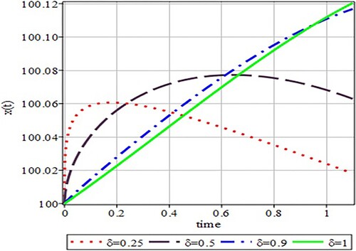
Figure 2. Behaviour of $y\left(t\right)$ for different values of $\delta$, showing infected CD4⁺ T-cells’ dynamics.

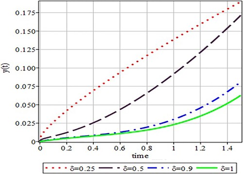
Figure 3. Behaviour of $z\left(t\right)$ for different values of $\delta$, showing dynamics of virions’ density.

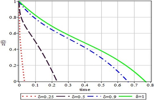
Table 1. Absolute errors for $x\left(t\right).$

t	$\delta$	$\text{VPM}$	$\text{VIM}$	$\text{HPM}$	$\text{ADM}$
0.02	0.25	8.8202E − 03	8.3675E − 03	8.3599E − 03	1.0443E − 01
	0.90	5.5299E − 05	9.0066E − 07	8.9583E − 07	8.3631E − 03
	1.00	2.1400E − 05	2.0000E − 07	2.0000E − 07	5.4397E − 03
0.06	0.25	1.0700E − 02	1.9077E − 02	1.9057E − 02	1.2936E − 01
	0.90	3.8839E − 04	1.7413E − 05	1.7396E − 05	2.2463E − 02
	1.00	1.8860E − 04	5.2000E − 06	5.2000E − 06	1.6314E − 02
0.10	0.25	1.0461E − 02	2.7986E − 02	2.7953E − 02	1.4067E − 01
	0.90	9.4855E − 04	6.9151E − 05	6.9094E − 05	3.5531E − 02
	1.00	5.1420E − 04	2.4100E − 05	2.4100E − 05	2.7174E − 02

Table 2. Absolute errors for $y\left(t\right)$.

t	$\delta$	$\text{VPM}$	$\text{VIM}$	$\text{HPM}$	$\text{ADM}$
0.02	0.25	9.5628E − 03	9.5644E − 03	9.5567E − 03	9.5668E − 03
	0.90	1.0246E − 06	1.0248E − 06	1.0241E − 06	1.0622E − 06
	1.00	2.2025E − 07	2.2029E − 07	2.2013E − 07	2.3478E − 07
0.06	0.25	2.1801E − 02	2.1806E − 02	2.1785E − 02	2.1801E − 02
	0.90	1.9898E − 05	1.9901E − 05	1.9887E − 05	2.0161E − 05
	1.00	5.9470E − 06	5.9480E − 06	5.9435E − 06	6.0747E − 06
0.10	0.25	3.1980E − 02	3.1989E − 02	3.1955E − 02	3.1976E − 02
	0.90	7.9035E − 05	7.9047E − 05	7.8988E − 05	7.9669E − 05
	1.00	2.7533E − 05	2.7538E − 05	2.7516E − 05	2.7879E − 05

Table 3. Absolute errors for $z\left(t\right)$.

t	$\delta$	$\text{VPM}$	$\text{VIM}$	$\text{HPM}$	$\text{ADM}$
0.02	0.25	8.0117E − 01	8.0117E − 01	8.0111E − 01	8.0111E − 01
	0.90	8.5870E − 05	8.5870E − 05	8.5870E − 05	8.5870E − 05
	1.00	1.8459E − 05	1.8459E − 05	1.8459E − 05	1.8459E − 05
0.06	0.25	1.8263E + 00	1.8263E + 00	1.8261E + 00	1.8261E + 00
	0.90	1.6675E − 03	1.6675E − 03	1.6675E − 03	1.6675E − 03
	1.00	4.9839E − 04	4.9839E − 04	4.9838E − 04	4.9838E − 04
0.10	0.25	2.6790E + 00	2.6790E + 00	2.6787E + 00	2.6787E + 00
	0.90	6.6232E − 03	6.6232E − 03	6.6231E − 03	6.6231E − 03
	1.00	2.3074E − 03	2.3074E − 03	2.3073E − 03	2.3073E − 03

5. Conclusion

We applied approximate analytical methods such as the VPM, VIM, HPM and ADM to solve the fractional-order model of HIV-1 infection of CD4⁺ T-cells comprising the effect of the anti-viral drug therapy. The proposed work contains the approximate solutions, showing the memory patterns of uninfected CD4⁺ T-cells, infected CD4⁺ T-cells and the density of virions in plasma, which could be helpful in predicting the improvements for the treatment of AIDS. The proposed methods reflect high accuracy for fractional orders: $0.25,0.5,0.9$ and the classical one is $\delta =1$. The overall performance of the employed methods shows their efficacy, simplicity, and the approach is straightforward. These methods can be very promising for a wide class of fractional-order systems of the applied nature.

Disclosure statement

No potential conflict of interest was reported by the authors.

References

- Podlubny I. Fractional differential equations: applications. Vol. 198. San Diego: Academic Press Inc; 1999. p. 1–340.
- Baleanu D, Jajarmi A, Hajipour M. On the nonlinear dynamical systems within the generalized fractional derivatives with Mittag–Leffler kernel. Nonlinear Dyn. 2018;94(1):397–414.
- Mainardi F. Fractional calculus and waves in linear viscoelasticity. London: Imperrial College Press; 2014.
- Alsaedi A, Nieto JJ, Venktesh V. Fractional electrical circuits. Adv Mech Eng. 2015;7(12):1–7.
- Khan U, Ellahi R, Khan R, et al. Extracting new solitary wave solutions of Benny-Luke equation and Phi-4 equation of fractional order by using (G'/G)-expansion method. Opt Quant Electron. 2017;49:362.
- Rahmatullah ER, Mohyud-din ST, Khan U. Exact traveling wave solutions of fractional order Boussinesq-like equations by applying Exp-function method. Results in Physics. 2018;8:114–120.
- Rocha D, Silva C J, Torres DFM. Stability and optimal control of a delayed HIV model. Math Methods Appl Sci. 2016;41(6):2251–2260.
- Perelson AS, Ribeiro RM. Modeling the within-host dynamics of HIV infection. BMC Biol. 2013;11:96.
- Wang S, Hottz P, Schechter M, et al. Modeling the slow CD4+ T cell decline in HIV-infected individuals. PLoS Comput Biol. 2015;11(12):1–25.
- Weiss RA. How does HIV cause AIDS? Science. 1993;260:1273–1279.
- Bonhoeffer S, Coffin JM, Nowak MA. Human immunodeficiency virus drug therapy and virus load. J Virol. 1997;71(4):3275–3278.
- Tuckwell HC. Nature of equilibria and effects of drug treatments in some simple viral population dynamical models. Math Med Biol. 2000;17(4):311–327.
- Arafa AAM, Rida SZ, Khalil M. The effect of anti-viral drug treatment of human immunodeficiency virus type 1 (HIV-1) described by a fractional order model. Appl Math Model. 2013;37(4):2189–2196.
- Pinto CMA, Carvalho ARM. A latency fractional order model for HIV dynamics. J Comput Appl Math. 2017;312:240–256.
- Yan Y, Kou C. Stability analysis for a fractional differential model of HIV infection of CD4+ CD4+ T-cells with time delay. Math Comput Simul. 2012;82(9):1572–1585.
- Ding Y, Ye H. A fractional-order differential equation model of HIV infection of CD4+ T-cells. Math Comput Model. 2009;50(3):386–392.
- Jajarmi A, Baleanu D. A new fractional analysis on the interaction of HIV with CD4 + T-cells. Chaos Solit Fractals. 2018;113:221–229.
- Arafa AAM, Rida SZ, Khalil M. Fractional modeling dynamics of HIV and CD4 + T-cells during primary infection. Nonlinear Biomed Phys. 2012;6(1):1–7.
- Gandomani MR, Kajani MT. Numerical solution of a factional order model of HIV infection of CD4 + T cells using Müntz-Legendre polynomials. Int J Bioautomation. 2016;20(2):193–204.
- Rahman JU, Lu D, Hui YS, et al. Numerical investigation of fractional HIV model using Elzaki pojected differential transform method. Fractals. 2018;26(5):1850062.
- Mohyud-Din ST, Yildirim A. Ma’s variation of parameters method for fisher’s equations. Adv Appl Math Mech. 2010;2(3):379–388.
- Mohyud-Din ST, Ahmed N, Waheed A, et al. Solutions of fractional diffusion equations by variation of parameters method. Therm. Sci. 2015;19:69–75.
- Mohyud-Din ST, Noor MA, Waheed A. Variation of parameters method for solving sixth-order boundary value problems. Commun Korean Math Soc. 2009;24(4):605–615.
- Molliq RY, Noorani MSM, Hashim I. Variational iteration method for fractional heat- and wave-like equations. Nonlinear Anal Real World Appl. 2009;10(3):1854–1869.
- Odibat ZM, Momani S. Application of variational iteration method to nonlinear differential equations of fractional orde. Int J Nonlinear Sci Numer Simul. 2006;7(1):27–34.
- Sontakke BR, Shelke AS, Shaikh AS. Solution of non-linear factional differential equations by variational iteration method and applications. Far East J Math Sci. 2019;110(1):113–129.
- Momani S, Odibat Z. Homotopy perturbation method for nonlinear partial differential equations of fractional order. Phys Lett A. 2007;365(5):345–350.
- He JH. Homotopy perturbation technique. Comput Methods Appl Mech Eng. 1999;178(3):257–262.
- Tripathi D. Numerical and analytical simulation of peristaltic flows of generalized Oldroyd-B fluids. Int J Numer Methods Fluids. 2011;67(12):1932–1943.
- Tripathi D. Peristaltic transport of fractional Maxwell fluids in uniform tubes: applications in endoscopy. Comput Math Appl. 2011;62(3):1116–1126.
- Tripathi D. Numerical study on peristaltic flow of generalized burgers’ fluids in uniform tubes in the presence of an endoscope. Int J Numer Meth Biomed Eng. 2011;27(11):1812–1828.
- Abbas MA, Bai YQ, Bhatti MM, et al. Three dimensional peristaltic flow of hyperbolic tangent fluid in non-uniform channel having flexible walls. Alexandria Eng J. 2016;55(1):653–662.
- Abdelsalam SI, Bhatti MM. The study of non-Newtonian nanofluid with hall and ion slip effects on peristaltically induced motion in a non-uniform channel. RSC Adv. 2018;8(15):7904–7915.
- Abdelsalam SI, Bhatti MM. The impact of impinging TiO2 nanoparticles in Prandtl nanofluid along with endoscopic and variable magnetic field effects on peristaltic blood flow. Multidiscip Model Mater Struct. 2018;14(3):530–548.
- Zeeshan A, Bhatti MM, Akbar NS, et al. Hydromagnetic blood flow of Sisko fluid in a non-uniform channel induced by peristaltic wave. Commun Theor Phys. 2017;68(1):103–110.
- Shawagfeh NT. The decomposition method for fractional differential equations. J Fract Calc. 1999;16:27–33.
- Danesh M, Safari M. Application of adomian’s decomposition method for the analytical solution of space fractional diffusion equation. Adv Pure Math. 2011;1(6):345–350.
- Bakkyaraj T, Sahadevan R. An approximate solution to some classes of fractional nonlinear partial differential using adomian decomposition method. J Fract Calc Appl. 2014;5(1):37–52.
- Adomian G. Solving frontier problems of physics: the decomposition method. Amsterdam: Springer Netherlands; 1994.
- Beg OA, Tripathi D, Sochi T, et al. Adomian decomposition method (ADM) simulation of magneto-bio-tribological squeeze film with magnetic induction effects. J Mech Med Biol. 2015;15(5):1550072.
- Shah K, Tunç C. Existence theory and stability analysis to a system of boundary value problem. J Taibah Univ Sci. 2017;11(6):1330–1342.
- Tunç C, Tunç O. Qualitative analysis for a variable delay system of differential equations of second order. J Taibah Univ Sci. 2019;13(1):468–477.
- Ellahi R, Hussain F, Ishtiaq F, et al. Peristaltic transport of Jeffrey fluid in a rectangular duct through a porous medium under the effect of partial slip: an approach to upgrade industrial sieves/filters. Pramana – J Phys. 2019;93:34.
- Zeeshan A, Shehzad N, Abbas T, et al. Effects of radiative electro-magnetohydrodynamics diminishing internal energy of pressure-driven flow of titanium dioxide-water nanofluid due to entropy generation. Entropy. 2019;21:36.
- Sohail A, Maqbool K, Ellahi R. On space spectral time fractional adam bashforth moulton method along with stability analysis for fractional order partial differential equations. Numer Methods Partial Differ Equ. 2018;34(1):19–29.
- Sarafraz MM, Pourmehran O, Yang B, et al. Pool boiling heat transfer characteristics of iron oxide nano-suspension under constant magnetic field. Int J Therm Sci. 2020;147:106131.
- Ellahi R, Sait SM, Shehzad N, et al. Numerical simulation and mathematical modeling of electroosmotic Couette-Poiseuille flow of MHD power-law nanofluid with entropy generation. Symmetry (Basel). 2019;11(8):1038.
- Alamri SZ, Khan AA, Azeez M, et al. Effects of mass transfer on MHD second grade fluid towards stretching cylinder: A novel perspective of Cattaneo–christov heat flux model. Phys Lett A. 2019;383:276–281.
- Alamri SZ, Ellahi R, Shehzad N, et al. Convective radiative plane Poiseuille flow of nanofluid through porous medium with slip: An application of Stefan blowing. J Mol Liq. 2019;273:292–304.
- Ellahi R, Alamri SZ, Basit A, et al. Effects of MHD and slip on heat transfer boundary layer flow over a moving plate based on specific entropy generation. J Taibah Univ Sci. 2018;12(4):476–482.
- Lichae BH, Biazar J, Ayati Z. The fractional differential model of HIV-1 infection of CD4 + T-cells with description of the effect of antiviral drug treatment. Comput Math Methods Med. 2019;2019:4059549.
- Caputo M. Linear models of dssipation whose Q is almost frequency independent-II. Geophys. J. R. Astron. Soc. 1967;13(5):529–539.
- Tuckwell HC, Wan FYM. On the behavior of solutions in viral dynamical models. BioSystems. 2004;73(3):157–161.