Estimation of multicomponent stress-strength reliability following Weibull distribution based on upper record values

ABSTRACT

Stress-strength models are of special importance in reliability literature and engineering applications. This paper deals with the estimation problem of a stress-strength model incorporating multi-component system. The system is regarded as alive only if at least $\mathcal{S}$ out of $k$ $(\mathcal{S}<k)$ strength components exceed the stress. The reliability of such system is obtained when strength and stress variables have Weibull distributions. Maximum likelihood estimator of $R_{\mathcal{S},k}$ and asymptotic confidence intervals are obtained based on upper record values. Bayesian estimator under squared error and linear exponential loss functions using gamma prior distributions and the corresponding credible intervals are obtained. Due to the lack of explicit forms for the Bayes estimates, the Markov Chain Monte Carlo (MCMC) method is employed. A simulation study is implemented to assess the performance of estimates. A real-life example is presented to show how the proposed model may be utilized in breaking strength of jute fibre data.

KEYWORDS:

• Weibull distribution
• multicomponent stress–strength reliability
• upper record values
• asymptotic confidence interval
• Markov Chain Monte Carlo

1. Introduction

Record values can be viewed as order statistic from a sample whose size is determined by the values and the order of occurrence of the observations. Record values and associated statistics have an important role in many real-life applications involving data related to meteorology, hydrology, sports and life tests. In industry and reliability, many products may fail under stress. For example, a wooden beam breaks when sufficient perpendicular force is applied to it, a battery dies under the stress of time, an electronic component ceases to function in an environment of too high temperature. In such experiments for getting the precise failure point, measurements may be made sequentially and only values larger (or smaller) than all previous ones are recorded. Data of this type are called record data. The development of the general theory of statistical analysis of record values began with the work, as pioneered in Chandler [1]. For an excellent review of records and their properties, one may refer to Nagaraja [2], Ahsanullah [3], Ahsanullah [4].

Let $X_1,X_2,\dots$ be an infinite sequence of identically independent distributed (IID) random variables with probability density function $f\left(x\right)$ and cumulative distribution function $F\left(x\right).$ Then, an observation $X_i$ is said to be an upper record value if it exceeds all its previous observations, i.e. $X_i>X_j$ for every $i<j.$ An analogous definition can be given for a lower record value.

The stress-strength reliability of a system defines the probability that the system will function properly until the strength exceeds the stress. Due to the manufacturing variability and uncertain factors, the strength of the system varies also when the system is put to use, it is subjected to the stress which is again random in nature. These manufacturing variables and uncertain factors can be used material, production style, humidity, temperature of the environment, etc. The genesis of this problem can be seen in Birnbaum [5]. Many authors have been interested in estimating a single component stress-strength version based on record values due to its important role in many fields. The survival probability of stress-strength $R=P\left(Y<X\right)$ based on record values is considered in Baklizi [6] for generalized exponential distribution. Subsequent papers extended this work assuming various lifetime distributions for stress-strength random variables, for instance, in Baklizi [7,8,9], for one and two parameter exponential distribution, Essam [10] for type I generalized logistic distribution, Baklizi [11] for two-parameter Weibull distribution, Tarvirdizade and Kazemzadeh Garehchobogh [12] for inverse Rayleigh distribution, Al-Gashgari and Shawky [13] for exponentiated Weibull distribution, Hassan et al. [14] for exponentiated inverted Weibull distribution and Hassan et al. [15] for generalized inverted exponential distribution.

Bhattacharyya and Johnson [16] observed that, in several practical scenarios, the performance of a system depends on more than one component and these components have their own strengths. Multicomponent stress-strength (MSS) models have great applications range from communication and industrial systems to logistic and military systems. For examples, an aircraft generally contains more than one engines (k) and assume that for takeoff at least $\mathcal{S}$ (1 ≤  $\mathcal{S}$  ≤ k) engines are needed. So, the aircraft will take off smoothly, if $\mathcal{S}$ out of k engines work; in engineering, a power system powering a manufacturing unit has k fuse cut-outs arranged in a parallel way. The power system will keep powering the manufacturing unit as long as at least $\mathcal{S}$ (1 ≤  $\mathcal{S}$  ≤ k) fuse cut-outs are working. Also, consider an automobile with a V-8 engine that works if four cylinders are rung. So, it can be represented as 4-out-of-8: G system. In suspension bridges, the deck is supported by a series of vertical cables hung from the towers. Suppose a suspension bridge consists of k number of vertical cable pairs. The bridge will only survive if a minimum $\mathcal{S}$ number of vertical cables through the deck are not damaged when subjected to stresses due to 153 American Journal of Applied Mathematics and Statistics wind loading, heavy traffic, corrosion etc. For extensive $\mathcal{S}$ out of k and related systems one may refer to Kuo and Zuo [17].

A multicomponent system of $k$ components having strengths following $k-$ IID random variables $X_1,X_2,\dots ,X_k$ and each component experiences a random stress Y. The system is regarded as alive only if at least $\mathcal{S}$ out of $k$ $(\mathcal{S}<k)$ strengths exceeds the stress. Let $X_1,X_2,\dots ,X_k$ be independent, $G\left(y\right)$ be the CDF of $Y$ and $F\left(x\right)$ be the common CDF of $X_1,X_2,\dots ,X_k$ . Then the reliability in the MSS model which is developed in Bhattacharyya and Johnson [16] is defined in the following form: (1) $\begin{array}{rl}{R}_{\mathcal{S},k}& =P\left[\text{at least }\mathcal{S}\text{of the }\left(X_1,X_2,\dots ,X_k\right)\text{ exceed }Y\right]\\ & =\sum _{i=\mathcal{S}}^k\left(\begin{array}{c}k\\ i\end{array}\right)\underset{-\mathrm{\infty }}{\overset{\mathrm{\infty }}{\int }}[1-F\left(y\right){]}^i[F\left(y\right){]}^{k-i}dG\left(y\right),\end{array}$(1) where $X_1,X_2,\dots ,X_k$ are IID with common distribution function $F\left(x\right)$ and subjected to the common random stress Y.

The applicability of the reliability in the MSS model based on the samples of upper record values appears strongly in industrial tests, where most of the systems fail when they are exposed to high levels of stress. For example, if a sample of electrical power stations consists of eight generating units, the light amount of electricity is generated if at least six generating units are operating. In some experimental energy tests, these power stations are exposed to a high level of stress in order to test its ability to carry out its functions (supply the region demand of electricity) at high levels of stress. It is expected that most of the systems of most of a lot of these power stations will collapse immediately under a high level of stress. If a few power stations can function for a short period of time under these high levels of stress, it will be recorded as a first observation to obtain the sample of the upper record values. If the longer period of time occurs, it will be recorded as a second observation and so on to obtain a sample of the upper record values.

Recently, several researchers have paid attention to develop inferential procedures for the reliability of MSS models. The reliability in the MSS model based on a simple random sample has been developed in Kuo and Zuo [17] and Pandey and Uddin [18]. A considerable amount of the literature on the estimation of reliability in the multicomponent system for some lifetime distributions has been studied by several authors; see for examples; Rao [19], Rao et al. [20], Rao [21], Kizilaslan and Nadar [22]. Recently, Pak et al. [23] investigated Bayesian estimation of the reliability of an MSS system for the bathtub-shaped distribution when the available data are reported in terms of record values. Jamal et al. [24] considered maximum likelihood and Bayesian estimation methods for MSS reliability for Pareto distribution based on the upper record values.

This article deals with the estimation of the MSS reliability defined in (1), the underline distribution of the strength and stress follows non-identical Weibull distribution when the considered data are of a record type. The expression for the reliability of the multicomponent system $R_{\mathcal{S},k}$ is obtained in Section 2. Maximum likelihood (ML) estimators are employed to obtain the asymptotic distribution and confidence intervals of $R_{\mathcal{S},k}$. Steps of numerical study and the corresponding results are given in Subsections 2.1 and 2.2, respectively. In Section 3, Bayesian estimators of $R_{\mathcal{S},k}$ are computed for a commonly known shape parameter $\text{β}$, and unknown parameters ${\lambda }_1$ and ${\lambda }_2$ as well as the highest posterior density credible intervals are also constructed. The MCMC method is employed under squared error (SE) and linear exponential (LINEX) loss functions for independent gamma priors in Subsection 3.1. Numerical results are outlined in Subsection 3.2. Real data are employed to assess the theoretical results in Section 4. Finally, concluding remarks appear in Section 5.

2. Maximum likelihood estimator of $R_{\mathcal{S},k}$

The Weibull distribution is a very popular distribution that has been extensively used over the past decades for modelling data in reliability, engineering and biological studies. It has numerous varieties of shapes and demonstrates considerable flexibility that enables it to have increasing, constant and decreasing failure rates. Therefore, it is used for many applications for example in hydrology, industrial engineering, weather forecasting and insurance. Weibull distribution is of special interest, because the Weibull distribution arises naturally from the extreme value theorem (Murthy et al. [25]) and thus it has a meaningful physical interpretation in many real applications (Ye et al. [26]). The probability density function (PDF) and cumulative distribution function (CDF) of the Weibull distribution are given as follows: (2) $f\left(x;\lambda ,\text{β}\right)=\lambda \text{β}{x}^{\text{β}-1}{e}^{-\lambda x^{\text{β}}},x,\lambda ,\text{and}\text{β}>0,$(2) and, (3) $F\left(x;\lambda ,\text{β}\right)=1-e^{-\lambda x^{\text{β}}}.x,\lambda ,\text{and}\text{β}>0.$(3)

Here, the ML estimator of the reliability in the MSS model based on upper record values is derived. Assuming that the strengths and stress random variables are independent, they are distributed as two-parameter Weibull distribution.

Let $X_1,X_2,\dots ,X_k$ be the strengths of a system which is subjected to the stress $Y$. Assuming that $X_1,X_2,\dots ,X_k$ be a random sample from Weibull distribution with parameters $\left({\lambda }_1,\text{β}\right)$ and $Y$ be a random variable from Weibull distribution with parameters $\left({\lambda }_2,\text{β}\right)$ are independent from unknown parameters ${\lambda }_1,{\lambda }_2$ and common shape parameter $\text{β}$ , respectively. Therefore, the reliability of $\mathcal{S}$ -out-of- $k$ system for Weibull distribution can be computed by using (1)–(3) as follows:

(4) $\begin{array}{rl}{R}_{\mathcal{S},k}& =\sum _{i=\mathcal{S}}^k\left(\begin{array}{c}k\\ i\end{array}\right)\underset{0}{\overset{\mathrm{\infty }}{\int }}{\lambda }_2\text{β}{y}^{\text{β}-1}{e}^{-\left({\lambda }_{1}i+\lambda \right)y^{\text{β}}}[1-e^{-{\lambda }_1{y}^{\text{β}}}{]}^{k-i}dy\\ & =\sum _{i=\mathcal{S}}^k\sum _{j=0}^{k-i}\left(\begin{array}{c}k\\ i\end{array}\right)\left(\begin{array}{c}k-i\\ j\end{array}\right)(-1{)}^j{\lambda }_2\underset{0}{\overset{\mathrm{\infty }}{\int }}{e}^{-\left({\lambda }_{1}i+{\lambda }_{1}j+{\lambda }_2\right)u}du.\end{array}$(4)

After the simplification, then $R_{\mathcal{S},k}$ will be (5) $R_{\mathcal{S},k}=\sum _{i=\mathcal{S}}^k\sum _{j=0}^{k-i}\left(\begin{array}{c}k\\ i\end{array}\right)\left(\begin{array}{c}k-i\\ j\end{array}\right)\frac{{(-1)}^j{\lambda }_2}{\left[{\lambda }_1\left(i+j\right)+{\lambda }_2\right]}.$(5)

In order to derive the ML estimator of ${\lambda }_1$ and ${\lambda }_2,$ let $\underset{\_}{r}=\left(r_0,r_1,\dots ,r_n\right)$ be a set of the first observed $\left(n+1\right)$ upper record values from Weibull distribution with parameters $\left({\lambda }_1,\text{β}\right)$ and $\underset{\_}{s}=\left(s_0,s_1,\dots ,s_m\right)$ be an independent set of the observed first $\left(m+1\right)$ upper record values from Weibull distribution with parameters $\left({\lambda }_2,\text{β}\right)$ where $\text{β}$ is assumed known. The likelihood function of the observed record values $\underset{\_}{r}$ and $\underset{\_}{s}$ is obtained, as follows: (6) $\begin{array}{rl}{L}_1\left({\lambda }_1,\text{β}|\underset{\_}{r}\right)& =f\left(r_n\right)\prod _{i=0}^{n-1}\frac{f\left(r_i\right)}{1-F\left(r_i\right)}\\ & =({\lambda }_1\text{β}{)}^{n+1}{e}^{-{\lambda }_1{r_n}^{\text{β}}}\prod _{i=0}^n{r_i}^{\text{β}-1}\end{array}$(6) and, (7) $\begin{array}{rl}{L}_2\left({\lambda }_2,\text{β}|\underset{\_}{s}\right)& =g\left(s_m\right)\prod _{j=0}^{m-1}\frac{g\left(s_i\right)}{1-G\left(s_i\right)}\\ & =({\lambda }_2\text{β}{)}^{m+1}{e}^{-{\lambda }_2{s_m}^{\text{β}}}\prod _{j=0}^m{s_j}^{\text{β}-1}\end{array}$(7)

Therefore, the joint log-likelihood function of the observed $\underset{\_}{r}$ and $\underset{\_}{s}$ denoted by $l$ takes the following form: (8) $\begin{array}{rl}l& =\left(n+1\right)ln{\lambda }_1+\left(m+1\right)ln{\lambda }_2\\ & +\left(n+m+2\right)ln\text{β}-{\lambda }_1{r_n}^{\text{β}}-{\lambda }_2{s_m}^{\text{β}}\\ & +\left(\text{β}-1\right)\left[\sum _{i=0}^n\ln \left(r_i\right)+\sum _{j=0}^m\ln \left(s_j\right)\right]\end{array}$(8) The ML estimator of ${\lambda }_1$ and ${\lambda }_2$, say ${\hat{\lambda }}_1$ and ${\hat{\lambda }}_2$ when $\text{β}$ assumed to known to be obtained by differentiating (8) and equating by zero. Then ${\hat{\lambda }}_1$ and ${\hat{\lambda }}_2$ take the following forms (9) ${\hat{\lambda }}_1=\frac{\left(n+1\right)}{{r_n}^{\text{β}}},{\hat{\lambda }}_2=\frac{\left(m+1\right)}{{s_m}^{\text{β}}}.$(9) Hence, the ML estimator of $R_{\mathcal{S},k}$, denoted by ${\hat{R}}_{\mathcal{S},k}$, is obtained by using (5) and (9) as follows: (10) ${\hat{R}}_{\mathcal{S},k}=\sum _{i=\mathcal{S}}^k\sum _{j=0}^{k-i}\left(\begin{array}{c}k\\ i\end{array}\right)\left(\begin{array}{c}k-i\\ j\end{array}\right)\frac{{(-1)}^j{\hat{\lambda }}_2}{\left[{\hat{\lambda }}_1\left(i+j\right)+{\hat{\lambda }}_2\right]}$(10)

Now to obtain the asymptotic confidence interval (ACI) for $R_{\mathcal{S},k},$ firstly, the asymptotic variance (AV) of the ML estimator is obtained as follows: (11) $\frac{\mathrm{\partial }{R}_{\mathcal{S},k}}{\mathrm{\partial }{\lambda }_1}=\sum _{i=\mathcal{S}}^k\sum _{j=0}^{k-i}\left(\begin{array}{c}k\\ i\end{array}\right)\left(\begin{array}{c}k-i\\ j\end{array}\right)\frac{{(-1)}^{j+1}\left(i+j\right){\lambda }_2}{{\left[{\lambda }_1\left(i+j\right)+{\lambda }_2\right]}^2},$(11) and, (12) $\frac{\mathrm{\partial }{R}_{\mathcal{S},k}}{\mathrm{\partial }{\lambda }_2}=\sum _{i=\mathcal{S}}^k\sum _{j=0}^{k-i}\left(\begin{array}{c}k\\ i\end{array}\right)\left(\begin{array}{c}k-i\\ j\end{array}\right)\frac{{(-1)}^j\left(i+j\right){\lambda }_1}{{\left[{\lambda }_1\left(i+j\right)+{\lambda }_2\right]}^2}.$(12)

The AV of an estimate of $R_{\mathcal{S},k}$ which is a function of two independent statistics ${\hat{\lambda }}_1$ and ${\hat{\lambda }}_2$ is given in Hassan and Basheikh [27]. (13) ${{\hat{\sigma }}^2}_{R_{s,k}}={\left[\frac{\mathrm{\partial }{R}_{s,k}}{\mathrm{\partial }{\lambda }_1}\right]}^{2}V\left({\hat{\lambda }}_1\right)+{\left[\frac{\mathrm{\partial }{R}_{s,k}}{\mathrm{\partial }{\lambda }_2}\right]}^{2}V\left({\hat{\lambda }}_2\right)$(13)

In this work, to avoid the difficulty in deriving $R_{\mathcal{S},k},$ we obtain AV for $\left(\mathcal{S},k\right)=\left(1,3\right)$ and (2,4) separately as follows: (14) $\begin{array}{rl}AV\left({\hat{R}}_{1,3}\right)& ={{\hat{\sigma }}^2}_{R_{1,3}}={\left[\frac{3{\hat{\lambda }}_2}{{\left[{\hat{\lambda }}_1+{\hat{\lambda }}_2\right]}^2}+\frac{6{\hat{\lambda }}_2}{{\left[2{\hat{\lambda }}_1+{\hat{\lambda }}_2\right]}^2}\right]}^2\frac{{{\hat{\lambda }}_1}^2}{n+1}\\ & +{\left[\frac{3{\hat{\lambda }}_1}{{\left[{\hat{\lambda }}_1+{\hat{\lambda }}_2\right]}^2}-\frac{6{\hat{\lambda }}_1}{{\left[2{\hat{\lambda }}_1+{\hat{\lambda }}_2\right]}^2}\right]}^2\frac{{{\hat{\lambda }}_2}^2}{m+1}\end{array}$(14) (15) $\begin{array}{rl}AV\left({\hat{R}}_{2,4}\right)={{\hat{\sigma }}^2}_{R_{2,4}}& =\left[\frac{-12{\hat{\lambda }}_2}{{\left[2{\hat{\lambda }}_1+{\hat{\lambda }}_2\right]}^2}+\frac{24{\hat{\lambda }}_2}{{\left[3{\hat{\lambda }}_1+{\hat{\lambda }}_2\right]}^2}\right.\\ & {\left.-\frac{8{\hat{\lambda }}_2}{{\left[4{\hat{\lambda }}_1+{\hat{\lambda }}_2\right]}^2}\right]}^2\frac{{{\hat{\lambda }}_1}^2}{n+1}\\ & +\left[\frac{12{\hat{\lambda }}_1}{{\left[2{\hat{\lambda }}_1+{\hat{\lambda }}_2\right]}^2}-\frac{24{\hat{\lambda }}_1}{{\left[3{\hat{\lambda }}_1+{\hat{\lambda }}_2\right]}^2}\right.\\ & {\left.+\frac{8{\hat{\lambda }}_1}{{\left[4{\hat{\lambda }}_1+{\hat{\lambda }}_2\right]}^2}\right]}^2\frac{{{\hat{\lambda }}_2}^2}{m+1}.\end{array}$(15) As n $\to \mathrm{\infty },m\to \mathrm{\infty }$ $\frac{{\hat{R}}_{\mathcal{S},k}-R_{\mathcal{S},k}}{AV\left({\hat{R}}_{\mathcal{S},k}\right)}\to N\left(0,1\right)$, therefore, an asymptotic $100\left[1-\alpha \right]\mathrm{\%}$ confidence interval of ${\hat{R}}_{\mathcal{S},k}$ for both $\left(\mathcal{S},k\right)=\left(1,3\right),\left(2,4\right)$ is given by (16) $\begin{array}{r}{R}_{\mathcal{S},k}\in {\hat{R}}_{\mathcal{S},k}\mp z_{\frac{\alpha }{2}}{\hat{\sigma }}_{R_{\mathcal{S},k}},\end{array}$(16) where $z_{\frac{\alpha }{2}}$ is the upper $\frac{\alpha }{2}th$ quantile of the standard normal distribution, ${\hat{\sigma }}_{R_{\mathcal{S},k}}$ is the value of ${\sigma }_{R_{\mathcal{S},k}}$ at the ML estimator, ${\hat{R}}_{\mathcal{S},k}-z_{\frac{\alpha }{2}}{\hat{\sigma }}_{R_{\mathcal{S},k}}$ is the lower limit of the confidence interval and ${\hat{R}}_{\mathcal{S},k}+z_{\frac{\alpha }{2}}{\hat{\sigma }}_{R_{\mathcal{S},k}}$ is the upper limit of the confidence interval.

2.1. Numerical study

In this subsection, an extensive numerical investigation is carried out to evaluate the performance of ML estimate (MLE) of $R_{\mathcal{S},k}$ at different values of ${\lambda }_1$ and ${\lambda }_2$ for different samples size of record values for the strengths and stress random variables. The performance of the point estimator depends mainly on the absolute biases (ABs) and mean square errors (MSEs). The length of intervals is the main principle of the performance of the ACI. The numerical study is designed through the following steps:

• Generate samples of the upper record values using some specified values of parameters.

• The values of ${\lambda }_1$ and ${\lambda }_2$ are selected as (3,1), (2.5,1.5), (2,1.5), (1.5,1.5), (1.5,2), (1.5,2.5),(1.5,3) and without loss of generality the value of $\text{β}$ is assumed to be known and equal to 3.

• The true values of reliability in the MSS model with the given combinations of $({\lambda }_1,{\lambda }_2)$ for $\left(\mathcal{S},k\right)=\left(1,3\right)$ are 0.54, 0.6, 0.67, 0.75, 0.82, 0.87 and 0.9, while the true values for $\left(\mathcal{S},k\right)=\left(2,4\right)$ are 0.39, 0.44, 0.51, 0.6, 0.69, 0.75 and 0.8, respectively.

• The samples of the upper record values of strength and stress random variables $\left(n,m\right)$ are chosen to be (10,10), (10,15), (15,10), (15,15), (15,20), (20,15) and (20,20).

• The MLEs of ${\lambda }_1$ and ${\lambda }_2$ are obtained from (9), then the MLE of $R_{\mathcal{S},k}$ is obtained by substituting ${\hat{\lambda }}_1$ and ${\hat{\lambda }}_2$ in (10).

• Compute the average ABs and average MSEs for reliability estimates over 5000 replications (see Tables 1–7).

• Obtain the asymptotic variance of $R_{1,3},$ $R_{2,4}$ by using (14) and (15), then compute the asymptotic standard deviation; ${\hat{\sigma }}_{R_{1,3}},{\hat{\sigma }}_{R_{2,4}}.$

• Compute the lower and upper limits of the ACI of $R_{1,3},$ $R_{2,4}$ through relation (16).

Table 1. The numerical results of MLE of $R_{\mathcal{S},k}$ at $\left({\lambda }_1,{\lambda }_2\right)=\left(3,1.5\right)$.

$\left(\mathcal{S},k\right)$	Exact $R_{\mathcal{S},k}$	$\left(n,m\right)$	AB	MSE	AL
(1, 3)	0.54	(10,10)	0.0710	0.0250	0.4960
		(10,15)	0.1660	0.0430	0.4230
		(15,10)	0.0310	0.0200	0.4560
		(15, 15)	0.0700	0.0220	0.4110
		(15,20)	0.1370	0.0320	0.3720
		(20,15)	0.0019	0.0140	0.3930
		(20, 20)	0.0770	0.0200	0.3600
(2,4)	0.39	(10,10)	0.0760	0.0240	0.4940
		(10,15)	0.1710	0.0470	0.4680
		(15,10)	0.0140	0.0150	0.4120
		(15, 15)	0.0750	0.0210	0.4070
		(15,20)	0.1460	0.0370	0.3940
		(20,15)	0.0082	0.0130	0.3580
		(20, 20)	0.0670	0.0180	0.3530

Table 2. The numerical results of the MLE of $R_{\mathcal{S},k}$ at $\left({\mathit{\lambda }}_1,{\mathit{\lambda }}_2\right)=\left(2.5,1.5\right)$.

$\left(\mathcal{S},k\right)$	Exact $R_{\mathcal{S},k}$	$\left(n,m\right)$	AB	MSE	AL
(1, 3)	0.6	(10,10)	0.0470	0.0220	0.4860
		(10,15)	0.1320	0.0330	0.4090
		(15,10)	0.0540	0.0230	0.4590
		(15, 15)	0.0470	0.0180	0.4060
		(15,20)	0.1100	0.0250	0.3600
		(20,15)	0.0250	0.0160	0.3910
		(20, 20)	0.0470	0.0160	0.3540
(2,4)	0.44	(10,10)	0.0670	0.0240	0.5050
		(10,15)	0.1610	0.0450	0.4630
		(15,10)	0.0370	0.0170	0.4270
		(15, 15)	0.0510	0.0200	0.4130
		(15,20)	0.1260	0.0310	0.3960
		(20,15)	0.0091	0.0140	0.3720
		(20, 20)	0.0570	0.0180	0.3620

Table 3. The numerical results of the MLE of $R_{\mathcal{S},k}$ at $\left({\mathit{\lambda }}_1,{\mathit{\lambda }}_2\right)=\left(2,1.5\right)$.

$\left(\mathcal{S},k\right)$	Exact $R_{\mathcal{S},k}$	$\left(n,m\right)$	AB	MSE	AL
(1, 3)	0.67	(10,10)	0.0210	0.0190	0.4700
		(10,15)	0.1090	0.0250	0.3760
		(15,10)	0.0780	0.0250	0.4590
		(15, 15)	0.0210	0.0160	0.3900
		(15,20)	0.0840	0.0180	0.3370
		(20,15)	0.0440	0.0160	0.3880
		(20, 20)	0.0290	0.0130	0.3400
(2,4)	0.51	(10,10)	0.0340	0.0210	0.5090
		(10,15)	0.1300	0.0340	0.4580
		(15,10)	0.0610	0.0210	0.4460
		(15, 15)	0.0340	0.0180	0.4210
		(15,20)	0.1060	0.0270	0.3910
		(20,15)	0.0360	0.0160	0.3840
		(20, 20)	0.0260	0.0150	0.3660

Table 4. The numerical results of the MLE of $R_{\mathcal{S},k}$ at $\left({\mathit{\lambda }}_1,{\mathit{\lambda }}_2\right)=\left(1.5,1.5\right)$.

$\left(\mathcal{S},k\right)$	Exact $R_{\mathcal{S},k}$	$\left(n,m\right)$	AB	MSE	AL
(1, 3)	0.75	(10,10)	0.0079	0.0150	0.4400
		(10,15)	0.0670	0.0150	0.3380
		(15,10)	0.1070	0.0280	0.4530
		(15, 15)	0.0089	0.0120	0.3660
		(15,20)	0.0450	0.0110	0.3070
		(20,15)	0.0730	0.0180	0.3740
		(20, 20)	0.0095	0.0099	0.3220
(2,4)	0.6	(10,10)	0.0017	0.0220	0.5020
		(10,15)	0.0910	0.0260	0.4340
		(15,10)	0.0900	0.0270	0.4620
		(15, 15)	0.0089	0.0160	0.4190
		(15,20)	0.0740	0.0200	0.3780
		(20,15)	0.0700	0.0200	0.3940
		(20, 20)	0.0010	0.0150	0.3650

Table 5. The numerical results of the MLE of $R_{\mathcal{S},k}$ at $\left({\mathit{\lambda }}_1,{\mathit{\lambda }}_2\right)=\left(1.5,2\right)$.

$\left(\mathcal{S},k\right)$	Exact $R_{\mathcal{S},k}$	$\left(n,m\right)$	AB	MSE	AL
(1, 3)	0.82	(10,10)	0.0350	0.0150	0.3990
		(10,15)	0.0350	0.0090	0.2910
		(15,10)	0.1250	0.0300	0.4340
		(15, 15)	0.0390	0.0130	0.3350
		(15,20)	0.0130	0.0079	0.2710
		(20,15)	0.0940	0.0210	0.3500
		(20, 20)	0.0340	0.0100	0.2900
(2,4)	0.69	(10,10)	0.0380	0.0210	0.4920
		(10,15)	0.0520	0.0180	0.4080
		(15,10)	0.1310	0.0370	0.4650
		(15, 15)	0.0320	0.0170	0.4080
		(15,20)	0.0310	0.0140	0.3590
		(20,15)	0.1060	0.0260	0.3960
		(20, 20)	0.0330	0.0140	0.3590

Table 6. The numerical results of the MLE of $R_{\mathcal{S},k}$ at $\left({\mathit{\lambda }}_1,{\mathit{\lambda }}_2\right)=\left(1.5,2.5\right)$.

$\left(\mathcal{S},k\right)$	Exact $R_{\mathcal{S},k}$	$\left(n,m\right)$	AB	MSE	AL
(1, 3)	0.87	(10,10)	0.0530	0.0140	0.3710
		(10,15)	0.0140	0.0062	0.2560
		(15,10)	0.1280	0.0310	0.4040
		(15,15)	0.0520	0.0120	0.3050
		(15,20)	0.0029	0.0056	0.2390
		(20,15)	0.1010	0.0210	0.3260
		(20,20)	0.0490	0.0110	0.2650
(2,4)	0.75	(10,10)	0.0630	0.0230	0.4750
		(10,15)	0.0250	0.0140	0.3800
		(15,10)	0.1550	0.0430	0.4650
		(15,15)	0.0520	0.0170	0.3920
		(15,20)	0.0078	0.0120	0.3340
		(20,15)	0.1230	0.0310	0.3890
		(20,20)	0.0560	0.0160	0.3440

Table 7. The numerical results of the MLE of $R_{\mathcal{S},k}$ at $\left({\mathit{\lambda }}_1,{\mathit{\lambda }}_2\right)=\left(1.5,3\right)$.

$\left(\mathcal{S},k\right)$	Exact $R_{\mathcal{S},k}$	$\left(n,m\right)$	AB	MSE	AL
(1, 3)	0.9	(10,10)	0.0630	0.0150	0.3400
		(10,15)	0.0007	0.0051	0.2300
		(15,10)	0.1310	0.0300	0.3830
		(15, 15)	0.0530	0.0100	0.2740
		(15,20)	0.0120	0.0047	0.2100
		(20,15)	0.1030	0.0200	0.3050
		(20, 20)	0.0530	0.0092	0.2410
(2,4)	0.8	(10,10)	0.0680	0.0220	0.4490
		(10,15)	0.0130	0.0120	0.3450
		(15,10)	0.1670	0.0460	0.4580
		(15, 15)	0.0750	0.0190	0.3790
		(15,20)	0.0170	0.0110	0.3190
		(20,15)	0.1300	0.0320	0.3770
		(20,20)	0.0680	0.0160	0.3270

2.2. Numerical results

Numerical results are reported in Tables 1–7 and represented through Figures 1–4. The following results can be observed on the properties of the reliability estimates as follows:

• The AB of ${\hat{R}}_{\mathcal{S},k}$ at $n=m$ increases as the value of ${\lambda }_1$ increases for both $\left(\mathcal{S},k\right)=\left(1,3\right)$ and $\left(2,4\right)$ [see Tables 1–3]. The AB of ${\hat{R}}_{\mathcal{S},k}$ at $n=m$ increases in the case of ${\lambda }_1\le {\lambda }_2$ in both $\left(\mathcal{S},k\right)=\left(1,3\right)$ and $\left(2,4\right)$ [see Tables 4–7].

• The MSEs of ${\hat{R}}_{\mathcal{S},k}$ for $\left(\mathcal{S},k\right)=\left(2,4\right)$ are almost larger than those for $\left(\mathcal{S},k\right)=\left(1,3\right)$ at different values of $\left({\lambda }_1,{\lambda }_2\right)$ included in Tables 1–7.

• For ${\lambda }_1>{\lambda }_2$, the MSEs of ${\hat{R}}_{\mathcal{S},k}$ for $n>m$ have values than the MSEs of ${\hat{R}}_{\mathcal{S},k}$ for $n<m$ in both $\left(\mathcal{S},k\right)$ in almost all cases. For ${\lambda }_1<{\lambda }_2$ the MSEs of ${\hat{R}}_{\mathcal{S},k}$ for $n<m$ have smaller values than those of ${\hat{R}}_{\mathcal{S},k}$ for $n>m$ in both $\left(\mathcal{S},k\right)$.

• For $n=m,$ the MSEs of ${\hat{R}}_{\mathcal{S},k}$ at ${\lambda }_1<{\lambda }_2$ have smaller values than those of ${\hat{R}}_{\mathcal{S},k}$ at ${\lambda }_1>{\lambda }_2$ in both $\left(\mathcal{S},k\right).$

• For $n=m,$ the MSEs of ${\hat{R}}_{\mathcal{S},k}$ for $\left(\mathcal{S},k\right)=\left(1,3\right)$ and $\left(2,4\right)$ decrease as $n$ and $m$ increase, at different values of ${\lambda }_1\text{ and}{\lambda }_2,$ [see for example Figure 1].

• For ${\lambda }_1<{\lambda }_2$ the average lengths (ALs) of ACI of ${\hat{R}}_{\mathcal{S},k}$ are less than the ALs of ACI of ${\hat{R}}_{\mathcal{S},k}$ when ${\lambda }_1>{\lambda }_2$ for both $\left(\mathcal{S},k\right),$ for different values of $n$ and $m$ .

• The ALs of ACI of ${\hat{R}}_{\mathcal{S},k}$ at $\left(\mathcal{S},k\right)=\left(1,3\right)$ are shorter than the corresponding ALs of ${\hat{R}}_{\mathcal{S},k}$ at $\left(\mathcal{S},k\right)=\left(2,4\right).$

• As seen in Tables 1–7, the ALs of ACI of ${\hat{R}}_{\mathcal{S},k}$ for $n=m$ are the tallest for different values of $\left({\lambda }_1,{\lambda }_2\right)$ in the case of $\left(\mathcal{S},k\right)=\left(2,4\right).$

• For $\left(n>m\right)$ and $\left(n<m\right)$ the MSEs of ${\hat{R}}_{\mathcal{S},k}$ tends to decrease as $n$ and $m$ increase for both $\left(\mathcal{S},k\right)$, at different values of ${\lambda }_1\text{and}{\lambda }_2$ , see for example Figures 2 and 3.

• At $\left(\mathcal{S},k\right)=\left(1,3\right),$ the ALs of ACI for ${\hat{R}}_{\mathcal{S},k}$ are the largest at $n=m,$ when ${\lambda }_1>{\lambda }_2.$

• At $\left(\mathcal{S},k\right)=\left(1,3\right),$ the largest ALs of ACI for ${\hat{R}}_{\mathcal{S},k}$ occur when $n>m$ in the case of ${\lambda }_1<{\lambda }_2$ .

• For $n=m,$ the ALs of ACI of ${\hat{R}}_{\mathcal{S},k}$ for both $\left(\mathcal{S},k\right)$ tends to decrease as $n$ and $m$ increase at different values of ${\lambda }_1\text{and}{\lambda }_2$ (see Figure 4).

• For $\left(n>m\right)$, and $\left(n<m\right)$, the ALs of ACI of ${\hat{R}}_{\mathcal{S},k}$ decrease as $n$ and $m$ increase for both $\left(\mathcal{S},k\right)$, at different values of ${\lambda }_1\text{and}{\lambda }_2.$

Figure 1. MSEs of ${\hat{R}}_{\mathcal{S},k}$ for different values of ${\lambda }_1,{\lambda }_2$ at $\left(\mathcal{S},k\right)=\left(1,3\right)$ in the case of $n=m$ .

Figure 2. MSEs of ${\hat{R}}_{\mathcal{S},k}$ for different values of ${\lambda }_1,{\lambda }_2$ at $\left(\mathcal{S},k\right)=\left(1,3\right)$ in the case of $n\ne m$ .

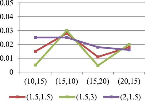
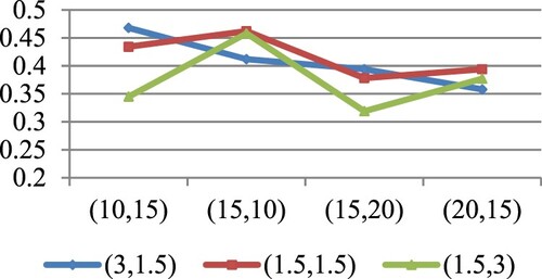
Figure 3. MSEs of ${\hat{R}}_{\mathcal{S},k}$ for different values of ${\lambda }_1,{\lambda }_2$ at $\left(\mathcal{S},k\right)=\left(2,4\right)$ in the case of $n=m$ .

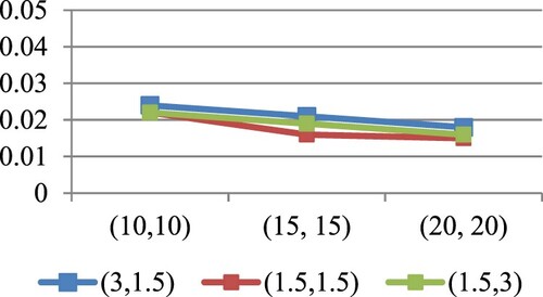
Figure 4. The ALs of ${\hat{R}}_{\mathcal{S},k}$ for different values of ${\lambda }_1,{\lambda }_2$ at $\left(\mathcal{S},k\right)=\left(2,4\right)$ in the case of $n\ne m$ .

3. Bayesian estimators of $R_{\mathcal{S},k}$

In this section, we assume that the parameters ${\lambda }_1$ and ${\lambda }_2$ are unknown and have independent gamma prior distributions with parameters $(a_i,b_i),$ i = 1, 2, respectively. Hence, assuming independence of parameters, the joint prior distribution of parameters, denoted by $\pi ({\lambda }_1,{\lambda }_2)$ is as follows: (16) $\begin{array}{rl}\pi ({\lambda }_1,{\lambda }_2)& =\frac{1}{\mathrm{\Gamma }\left(a_1\right)\mathrm{\Gamma }\left(a_2\right)}{\lambda }_1^{a_1-1}{\lambda }_2^{a_2-1}\\ & e^{-b_1{\lambda }_1-b_2{\lambda }_2},a_1,a_2,b_1,b_2,{\lambda }_1,{\lambda }_2>0.\end{array}$(16)

Based on the observed sample, the joint density function of ${\lambda }_1\text{and}{\lambda }_2$ and the data are (17) $\begin{array}{rl}& \pi ({\lambda }_1,{\lambda }_2,\underset{\_}{s},\underset{\_}{r})\\ & =\frac{1}{\mathrm{\Gamma }\left(a_1\right)\mathrm{\Gamma }\left(a_2\right)}{\lambda }_1^{a_1+n}{\lambda }_2^{a_2+m}\\ & e^{-{\lambda }_1\left(b_1+{r_n}^{\text{β}}\right)-{\lambda }_2\left(b_2+{s_m}^{\text{β}}\right)}{\text{β}}^{m+n+2}\prod _{i=0}^n{r_i}^{\text{β}-1}\prod _{j=0}^m{s_j}^{\text{β}-1}\end{array}$(17)

Thus, we can write the posterior density function of ${\lambda }_1\text{and}{\lambda }_2$ as (18) ${\pi }^{\ast }({\lambda }_1,{\lambda }_2|\underset{\_}{s},\underset{\_}{r})=\frac{\pi ({\lambda }_1,{\lambda }_2,\underset{\_}{s},\underset{\_}{r})}{{\int }_0^{\mathrm{\infty }}{\int }_0^{\mathrm{\infty }}\pi ({\lambda }_1,{\lambda }_2,\underset{\_}{s},\underset{\_}{r})d{\lambda }_{1}d{\lambda }_2}.$(18)

It is well known that assuming SE loss function, the Bayesian estimator of $R_{\mathcal{S},k},$ denoted by ${\tilde{R}}_{\mathcal{S},k}$ is its posterior mean which is obtained by (19) ${\tilde{R}}_{\mathcal{S},k}=E(R_{\mathcal{S},k}|\underset{\_}{s},\underset{\_}{r})=\underset{0}{\overset{\mathrm{\infty }}{\int }}\underset{0}{\overset{\mathrm{\infty }}{\int }}{R}_{\mathcal{S},k}{\pi }^{\ast }({\lambda }_1,{\lambda }_2|\underset{\_}{s},\underset{\_}{r})d{\lambda }_{1}d{\lambda }_2$(19)

Additionally, the Bayesian estimator of $R_{\mathcal{S},k}$ under LINEX loss function, denoted by ${\stackrel{⃛}{R}}_{\mathcal{S},k}$ is given as follows: (20) $\begin{array}{rl}{\stackrel{⃛}{R}}_{\mathcal{S},k}& =\frac{-1}{\nu }logE\left(e^{-\nu R_{\mathcal{S},k}}\right)\\ & =\frac{-1}{\nu }log\left\{\underset{0}{\overset{\mathrm{\infty }}{\int }}\underset{0}{\overset{\mathrm{\infty }}{\int }}{e}^{-\nu R_{\mathcal{S},k}}{\pi }^{\ast }({\lambda }_1,{\lambda }_2|\underset{\_}{s},\underset{\_}{r})d{\lambda }_{1}d{\lambda }_2\right\},\\ & \nu \ne 0.\end{array}$(20)

Since the posterior density function ${\pi }^{\ast }({\lambda }_1,{\lambda }_2|\underset{\_}{s},\underset{\_}{r})$ has a complex form, it is difficult to derive a closed form for the Bayesian estimator of $R_{\mathcal{S},k}$. Therefore, the MCMC technique is used to approximate these integrations. Metropolis-Hastings (M-H) algorithm will be implemented to compute the Bayes estimates and credible intervals width under SE and LINEX loss functions.

3.1. MCMC method

In order to investigate the behaviour of the multicomponent reliability $R_{\mathcal{S},k}$, Monte Carlo simulation is carried out. The Bayes estimates are obtained using gamma priors under SE and LINEX loss functions. The Bayesian estimate performances of $R_{\mathcal{S},k}$ are measured based on ABs, estimated Risks (ERs) and ALs via R 3.4.3. Three sets of parameter values are considered as $\left({\lambda }_1,{\lambda }_2,\text{β}\right)=\left(3,1.5,3\right),\left(1.5,1.5,3\right),\left(1.5,2,3\right)$ and different choices of sample sizes as $\left(n,m\right)=\left(10,10\right),\left(10,15\right),\left(15,10\right),\left(15,15\right),\left(15,20\right),\left(20,15\right),\left(20,20\right)$. The true value for $\left(\mathcal{S},k\right)=\left(1,3\right)$ is 0.54, 0.75 and 0.82 and for $\left(\mathcal{S},k\right)=\left(2,4\right)$ is 0.39, 0.6 and 0.69. Three different sets of hyper-parameters values are considered as; Prior I: $\left(a_1,b_1\right),\left(a_2,b_2\right)=\left(4,1\right),\left(4,1\right)$; Prior II: $\left(a_1,b_1\right),\left(a_2,b_2\right)=\left(8,2\right),\left(2,1\right)$ and Prior III: $\left(a_1,b_1\right),\left(a_2,b_2\right)=\left(6,2\right),\left(5,1.5\right).$ Also, we take $(v=-2,2).$ All the results are based on the number of replications = 5000.

The M–H algorithm is one of the most famous subclasses of the MCMC method in the Bayesian literature to simulate the deviates from the posterior density and produce good approximate results. The major difficulty in the implementation of the Bayesian procedure is that of obtaining the posterior distribution. The MCMC is used to simulate samples from the posterior density and then obtain the Bayesian estimate ${\tilde{R}}_{\mathcal{S},\text{k}}$ under SE loss function and ${\stackrel{⃛}{R}}_{\mathcal{S},\text{k}}$ under LINEX loss function.

The approximate Bayes estimate of $R_{\mathcal{S},\text{k}}$ is obtained by applying the M-H algorithm technique. The M–H algorithm uses an acceptance/rejection rule to converge to the target distribution. According to Lynch [28], the M–H algorithm proceeds as follows:

• Step 1: Initialize a starting parameter value $R_{\mathcal{S},\text{k}}^0$ and determine the number of samples N.

• Step 2: For $i=2$ to N, set $R_{s,k}=R_{s,k}^{i-1}$ .

• Step 3: Generate $u$ from uniform(0,1).

• Step 4: Draw a candidate parameter $R_{\mathcal{S},\text{k}}^{\ast }$ from the proposal density.

• Step 5: If $u\le \frac{\pi \left({\theta }^{\ast }\right)g\left(\theta |{\theta }^{\ast }\right)}{\pi \left(\theta \right)g\left({\theta }^{\ast }|\theta \right)}$ then, set $R_{\mathcal{S},k}^i=R_{\mathcal{S},\text{k}}^{\ast }$ otherwise, set $R_{\mathcal{S},k}^i=R_{\mathcal{S},k}$ .

• Step 6: Set $i=i+1$ and return to step 2 and repeat the previous steps N times.

3.2. Simulated results

Here, the simulated outcomes are listed in Tables 8–10 and represented through Figures 5–8, so from these tables we detect the following observations about the performance of the reliability estimates as follows:

• The ER of $R_{\mathcal{S},\text{k}}$ under LINEX loss function at $v=-2$ is the smallest for $\left(\mathcal{S},k\right)=\left(1,3\right)$ while the ER of $R_{\mathcal{S},\text{k}}$ under LINEX loss function at $v=2$ is the smallest when $\left(\mathcal{S},k\right)=\left(2,4\right)$ for different values of $\left(n,m\right)$ for ( ${\lambda }_1,{\lambda }_2)=(3,1.5)$ using prior I, as shown in Figures 5 and 6 in most of the cases.

• The ER of ${\tilde{R}}_{\mathcal{S},k}$ under SE loss function takes the largest values in approximately most of the situations compared with the corresponding ER of ${\stackrel{⃛}{R}}_{\mathcal{S},\text{k}}$ under LINEX loss function (see Figures 5 and 6).

• The ER of ${\stackrel{⃛}{R}}_{\mathcal{S},\text{k}}$ at $v=2$ decreases for n and m greater than or equal to 15, while the ER of ${\stackrel{⃛}{R}}_{\mathcal{S},\text{k}}$ at $v=-2$ is the smallest for $\left(\mathcal{S},k\right)=\left(2,4\right)$ for most values of $\left(n,m\right)$ when $({\lambda }_1,{\lambda }_2)=\left(1.5,2\right)$ using prior III, as shown in Figure 7.

• The AL of ${\stackrel{⃛}{R}}_{\mathcal{S},\text{k}}$ at $v=2$ takes the larger value for $({\lambda }_1,{\lambda }_2)=\left(1.5,2\right),$ and $\left(\mathcal{S},k\right)=\left(1,3\right)$ compared to the corresponding SE and LINEX $(v=-2)$ loss functions using prior III, as shown in Figure 8.

Figure 5. ER of $R_{\mathcal{S},k}$ estimates for $({\lambda }_1,{\lambda }_2)=\left(3,1.5\right)$ at $\left(\mathcal{S},k\right)=\left(1,3\right)$ under SE and LINEX loss functions for prior I.

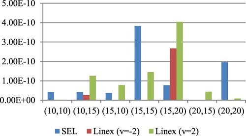
Figure 6. ER of $R_{\mathcal{S},k}$ estimates for $({\lambda }_1,{\lambda }_2)=\left(3,1.5\right)$ at $\left(\mathcal{S},k\right)=\left(2,4\right)$ under SE and LINEX loss functions for prior I.

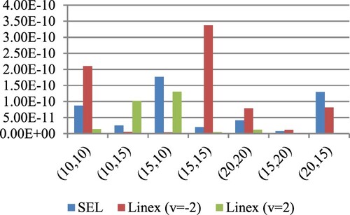
Figure 7. ER of $R_{\mathcal{S},k}$ estimates for $({\lambda }_1,{\lambda }_2)=\left(1.5,2\right)$ at $\left(\mathcal{S},k\right)=\left(2,4\right)$ under SE and LINEX loss functions for prior III.

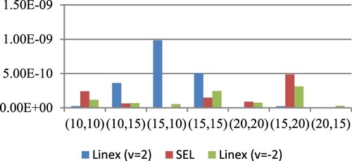
Figure 8. AL of $R_{\mathcal{S},k}$ estimates for $({\lambda }_1,{\lambda }_2)=\left(1.5,2\right)$ at $\left(\mathcal{S},k\right)=\left(1,3\right)$ under SE and LINEX loss functions for prior III.

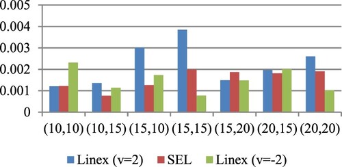
Table 8. AB, ER and AL of Bayes estimate of $R_{\mathcal{S},k}$ for prior I at$\left({\mathit{\lambda }}_1,{\mathit{\lambda }}_2\right)=\left(3,1.5\right)$.

$\left(\mathcal{S},k\right)=\left(1,3\right)$						$\left(\mathcal{S},k\right)=\left(2,4\right)$
Loss function	Exact $R_{\mathcal{S},k}$	(n, m)	AB	ER	AL	Exact $R_{\mathcal{S},k}$	AB	ER	AL
SE	0.54	(10,10)	0.00046	4.22E-11	0.0020	0.39	0.00066	8.73E-11	0.0030
LINEX (v = 2)			0.00000	2.88E-12	0.0014		0.00026	1.40E-11	0.0013
LINEX (v = −2)			0.00000	2.62E-12	0.0021		0.00103	2.10E-10	0.0029
SEL		(10,15)	0.00046	4.23E-11	0.0011		0.00036	2.55E-11	0.0035
LINEX (v = 2)			0.00000	1.26E-10	0.0020		0.00071	1.02E-10	0.0014
LINEX (v = −2)			0.00000	2.73E-11	0.0010		0.00016	5.30E-12	0.0014
SE		(15,10)	0.00043	3.75E-11	0.0013		0.00094	1.77E-10	0.0023
LINEX (v = 2)			0.00000	7.81E-11	0.0016		0.00081	1.31E-10	0.0024
LINEX (v = −2)			0.00000	4.59E-14	0.0012		0.00014	4.08E-12	0.0011
SE		(15,15)	0.00138	3.83E-10	0.0028		0.00032	2.09E-11	0.0012
LINEX (v = 2)			0.00000	1.45E-10	0.0014		0.00016	4.85E-12	0.0011
LINEX (v = −2)			0.00000	1.96E-12	0.0012		0.00130	3.38E-10	0.0023
SE		(15,20)	0.00062	7.76E-11	0.0013		0.00020	8.04E-12	0.0017
LINEX (v = 2)			0.00000	4.04E-10	0.0027		0.00000	1.48E-15	0.0019
LINEX (v = −2)			0.00000	2.67E-10	0.0017		0.00024	1.16E-11	0.0021
SE		(20,15)	0.00007	1.02E-12	0.0019		0.00081	1.30E-10	0.0018
LINEX (v = 2)			0.00000	4.37E-11	0.0008		0.00001	2.68E-14	0.0013
LINEX (v = −2)			0.00000	6.97E-13	0.0018		0.00064	8.17E-11	0.0018
SE		(20,20)	0.00099	1.97E-10	0.0024		0.00046	4.15E-11	0.0012
LINEX (v = 2)			0.00000	8.69E-12	0.0021		0.00024	1.20E-11	0.0013
LINEX (v = −2)			0.00000	7.75E-13	0.0010		0.00063	7.92E-11	0.0018

Table 9. AB, ER and AL of Bayes estimate of $R_{\mathcal{S},k}$ for prior II at $\left({\mathit{\lambda }}_1,{\mathit{\lambda }}_2\right)=\left(1.5,1.5\right)$.

$\left(\mathcal{S},k\right)=\left(1,3\right)$						$\left(\mathcal{S},k\right)=\left(2,4\right)$
Loss function	Exact $R_{\mathcal{S},k}$	(n, m)	AB	ER	AL	Exact $R_{\mathcal{S},k}$	AB	ER	AL
SE	0.75	(10,10)	0.0007	1.12E-12	0.0023	0.6	0.0006	3.17E-11	0.0015
LINEX (v = 2)			0.0004	1.31E-13	0.0015		0.0016	3.92E-10	0.0027
LINEX (v = −2)			0.0008	1.11E-10	0.0014		0.0004	1.33E-11	0.0009
SE		(10,15)	0.0011	1.67E-10	0.0020		0.0006	1.86E-11	0.0016
LINEX (v = 2)			0.0012	2.22E-10	0.0020		0.0005	3.93E-11	0.0009
LINEX (v = −2)			0.0011	1.42E-10	0.0020		0.0008	1.03E-10	0.0010
SE		(15,10)	0.0012	1.57E-10	0.0024		0.0010	1.55E-10	0.0017
LINEX (v = 2)			0.0013	2.83E-10	0.0020		0.0012	2.28E-10	0.0019
LINEX (v = −2)			0.0009	8.59E-11	0.0019		0.0006	8.78E-12	0.0018
SE		(15,15)	0.0006	1.47E-11	0.0019		0.0004	1.11E-11	0.0013
LINEX (v = 2)			0.0010	1.16E-10	0.0021		0.0010	1.41E-10	0.0022
LINEX (v = −2)			0.0007	1.08E-12	0.0027		0.0007	4.49E-11	0.0017
SE		(15,20)	0.0019	5.92E-10	0.0026		0.0015	4.14E-10	0.0017
LINEX (v = 2)			0.0011	1.62E-10	0.0020		0.0004	2.14E-11	0.0010
LINEX (v = −2)			0.0009	1.10E-10	0.0016		0.0009	1.06E-10	0.0021
SE		(20,15)	0.0003	1.26E-12	0.0012		0.0003	3.49E-12	0.0012
LINEX (v = 2)			0.0004	1.35E-11	0.0012		0.0017	3.90E-10	0.0030
LINEX (v = −2)			0.0018	4.35E-10	0.0029		0.0015	3.54E-10	0.0021
SE		(20,20)	0.0003	4.30E-12	0.0008		0.0012	1.42E-10	0.0027
LINEX (v = 2)			0.0009	9.34E-11	0.0020		0.0024	8.62E-10	0.0035
LINEX (v = −2)			0.0018	5.08E-10	0.0029		0.0014	2.70E-10	0.0025

Table 10. AB, ER and AL of Bayes estimate of $R_{\mathcal{S},k}$ for prior III at $\left({\lambda }_1,{\lambda }_2\right)=\left(1.5,2\right)$.

$\left(\mathcal{S},k\right)=\left(1,3\right)$						$\left(\mathcal{S},k\right)=\left(2,4\right)$
Loss function	Exact $R_{\mathcal{S},k}$	(n, m)	AB	ER	AL	Exact $R_{\mathcal{S},k}$	AB	ER	AL
SE	0.82	(10,10)	0.0003	1.71E-11	0.0012	0.69	0.0011	2.42E-10	0.0017
LINEX (v = 2)			0.0003	1.28E-11	0.0012		0.0004	2.49E-11	0.0018
LINEX (v = −2)			0.0012	3.04E-10	0.0023		0.0008	1.17E-10	0.0023
SE		(10,15)	0.0000	1.28E-13	0.0008		0.0006	6.36E-11	0.0018
LINEX (v = 2)			0.0000	1.83E-13	0.0014		0.0013	3.63E-10	0.0019
LINEX (v = −2)			0.0006	6.37E-11	0.0011		0.0006	6.85E-11	0.0011
SE		(15,10)	0.0005	5.49E-11	0.0013		0.0002	5.67E-12	0.0014
LINEX (v = 2)			0.0019	6.93E-10	0.0030		0.0022	9.82E-10	0.0031
LINEX (v = −2)			0.0007	1.01E-10	0.0017		0.0005	5.29E-11	0.0022
SE		(15,15)	0.0011	2.57E-10	0.0020		0.0009	1.48E-10	0.0018
LINEX (v = 2)			0.0023	1.10E-09	0.0039		0.0016	5.06E-10	0.0027
LINEX (v = −2)			0.0001	6.56E-13	0.0008		0.0011	2.47E-10	0.0015
SE		(15,20)	0.0007	1.08E-10	0.0019		0.0016	4.86E-10	0.0024
LINEX (v = 2)			0.0005	4.71E-11	0.0015		0.0003	2.32E-11	0.0010
LINEX (v = −2)			0.0010	1.95E-10	0.0015		0.0012	3.11E-10	0.0023
SE		(20,15)	0.0015	4.63E-10	0.0018		0.0002	8.23E-12	0.0018
LINEX (v = 2)			0.0012	2.70E-10	0.0020		0.0000	6.81E-16	0.0012
LINEX (v = −2)			0.0001	2.80E-12	0.0020		0.0004	3.13E-11	0.0016
SE		(20,20)	0.0012	2.76E-10	0.0019		0.0007	8.98E-11	0.0019
LINEX (v = 2)			0.0014	4.04E-10	0.0026		0.0001	3.16E-12	0.0010
LINEX (v = −2)			0.0004	3.07E-11	0.0010		0.0006	7.34E-11	0.0011

4. Real data application

In this section, the analysis of a pair of real data sets is presented for illustrative purposes. These two data sets were used by Xia et al. [29]. The data stand for the strength data measured in MPa, tensile properties of jute fibres were evaluated in accordance with ASTM C 1557–03 at seven different gauge lengths (2, 3, 5, 10, 15, 20, and 25 mm). Thirty samples were mounted for testing at each of these gauge lengths. We consider the data sets consisting of the breaking strength of jute fibre at 10 mm in gauge lengths, which represents the strength measurement (Data Set 1) and 20 mm in gauge lengths, which represents the stress measurement (Data Set 2), with sample sizes 30 each (see Tables 11–12).

Table 11. Data Set 1 (gauge lengths of 10 mm).

693.73	704.66	323.83	778.17	123.06	637.66	383.43
151.48	108.94	50.16	671.49	183.16	257.44	727.23
291.27	101.15	376.42	163.40	141.38	700.74	262.90
353.24	422.11	43.93	590.48	212.13	303.90	506.60
530.55	177.25

Table 12. Data Set 2 (gauge lengths of 20 mm).

71.46	419.02	284.64	585.57	456.6	113.85	187.85
688.16	662.66	45.58	578.62	756.7	594.29	166.49
99.72	707.36	765.14	187.13	145.96	350.7	547.44
116.99	375.81	581.6	119.86	48.01	200.16	36.75
244.53	83.55

The two data sets are fitted separately with the Weibull distribution using the Kolmogorov–Smirnov (K-S) goodness-of-fit test and the results are reported in Table 13.

Table 13. K-S goodness of fit and corresponding P-values for data sets 1 and 2.

	K-S	P-value
Data set 1	0.106	0.8899
Data set 2	0.149	0.51784

The K–S goodness of fit statistic and the corresponding P-value indicate that the Weibull distribution fits the data sets. From Tables 11 and 12, the upper record values are obtained as follows: $\begin{array}{r}\begin{array}{l}r=(693.73,704.66,778.17),\\ s=(71.46,419.02,585.57,688.16,756.7,765.14).\end{array}\end{array}$

Here, assuming two different choices $\left(\mathcal{S},k\right)$ for the MSS system, we compute the estimates of reliability parameter $R_{\mathcal{S},k},$ by using the ML and Bayesian procedures developed in the present paper. Using the above record values, the MLEs of the reliability, $R_{\mathcal{S},k}$ for $\left(\mathcal{S},k\right)$  = (1,3), (2,4), are 0.9 and 0.8, respectively.

To analyse the data from the Bayesian procedure, three different sets of values for the hyper-parameters are considered as Prior I: $\left(a_1,b_1\right),\left(a_2,b_2\right)=\left(4,1\right),\left(4,1\right)$; Prior II: $\left(a_1,b_1\right),\left(a_2,b_2\right)=\left(8,2\right),\left(2,1\right)$ and Prior III: $\left(a_1,b_1\right),\left(a_2,b_2\right)=\left(6,2\right),\left(5,1.5\right).$ Table 14 provides the Bayes estimates of $R_{\mathcal{S},k}$ under SE and LINEX loss functions. It is observed that the Bayes estimates obtained based on prior I, II and III are close to the MLEs at ( $\mathcal{S},k$ ) = (1,3) while employing $\left(\mathcal{S},k\right)$  = (2,4) leads to Bayes estimates are greater than the MLEs. Considering prior I and prior III, we conclude that the Bayes estimate of $R_{\mathcal{S},k}$ under LINEX at v = 2 is preferable to the other estimates. Regarding prior II, we conclude that the Bayes estimate of $R_{\mathcal{S},k}$ under SE is preferable to the other estimates. Generally, as the values of $\left(\mathcal{S},k\right)$ increase, the value of $R_{\mathcal{S},k}$ estimate decreases (see Table 14).

Table 14. The Bayes estimate of $R_{\mathcal{S},k}$ for the real data.

Prior	$\left(\mathcal{S},k\right)$	Loss function	$R_{\mathcal{S},k}$ estimate	$\left(\mathcal{S},k\right)$	$R_{\mathcal{S},k}$ estimate
I	(1,3)	SE	0.9899	(2,4)	0.9628
		LINEX (v = 2)	0.9975		0.9514
		LINEX (v = −2)	0.9832		0.9611
II	(1,3)	SE	0.9905	(2,4)	0.9688
		LINEX (v = 2)	0.9893		0.965
		LINEX (v = −2)	0.9784		0.9664
III	(1,3)	SE	0.9850	(2,4)	0.9688
		LINEX (v = 2)	0.9868		0.9665
		LINEX (v = −2)	0.9807		0.9704

5. Conclusion

This article concerns the estimation of multicomponent stress-strength reliability based on record data. The reliability of such a system is obtained when the strength and stress variables are independently Weibull distribution with different scale parameters. The reliability in MSS is estimated by using the maximum likelihood and Bayesian methods of estimation when the samples are drawn from strength and stress distributions and their measurements are in terms of the upper record values. The ML estimator is employed to obtain the asymptotic distribution and confidence intervals for $R_{\mathcal{S},k}.$ Considering SE and LINEX loss functions, all the Bayes estimates are computed by assuming gamma priors on the parameters. Since the Bayes estimates of the interested reliability parameter could not be obtained analytically, we employ the MCMC to obtain the Bayes estimates. To assess the accuracy of the different estimators, Monte Carlo simulations are conducted.

From the simulation study, we conclude that, the average bias and average MSE decrease as the sample size increases for both values of $\left(\mathcal{S},k\right)$. It verifies the consistency property of the MLE of $R_{\mathcal{S},k}.$ Also, the lengths of asymptotic confidence intervals of $R_{\mathcal{S},k}$ decrease as the sample size increases. Overall, the performance of the confidence interval is quite good for all combinations of parameters. Regarding the sizes of record value samples for the strengths and stress variables $\left(n,m\right),$ it is observed that the MSEs and the lengths of asymptotic confidence intervals tend to decrease as $\left(n,m\right)$ increases.

Regarding the MCMC method, we conclude that the estimated risk of prior I under SE loss function takes the smallest value at $\left(\mathcal{S},k\right)=\left(2,4\right)$, while the estimated risk under LINEX $\left(v=-2,2\right)$ takes the smallest value at $\left(\mathcal{S},k\right)=\left(1,3\right)$ among other priors in most of the situations. The AB of prior I has the smallest value under SE and LINEX $(v=2)$ at $\left(\mathcal{S},k\right)=\left(2,4\right),$ while the AB gets the smallest value for LINEX $\left(v=-2\right)$ at $\left(\mathcal{S},k\right)=\left(1,3\right)$ among other priors in most of the cases. Generally, prior I is preferable to prior II and III in approximately most of the situations due to their absolute biases and estimated risks values. Finally, the application to real data shows that the reliability estimates approach one for this model which indicates its importance in practice.

Disclosure statement

No potential conflict of interest was reported by the author(s).

References

- Chandler KN. The distribution and frequency of record values. J Royal Stat Soc Series B. 1952;14(2):220–228. DOI:10.1111/j.2517-6161.1952.tb00115.x.
- Nagaraja HN. Record values and related statistics. Commun Stat Theory Methods. 1988;17(7):2223–2238. DOI: 10.1080/03610928808829743.
- Ahsanullah M. Record statistics. Commack: Nova Science Publishers; 1995.
- Ahsanullah M. Record values-theory and applications. Lanham: University Press of America; 2004.
- Birnbaum Z. On a use of the Mann-Whitney statistic. Proceedings of the Third Berkeley Symposium on Mathematical Statistics and Probability, Volume 1: Contributions to the Theory of Statistics; 1956. The Regents of the University of California. DOI:10.1007/978-3-642-04898-2_615.
- Baklizi A. Likelihood and Bayesian estimation of Pr(X < Y) using lower record values from the generalized exponential distribution. Comput Stat Data Anal. 2008;52(7):3468–3473. DOI:10.1016/j.csda.2007.11.002.
- Baklizi A. Estimation of Pr(X < Y) using record values in the one and two parameter exponential distributions. Commun Stat Theory Methods. 2008;37(5):692–698. DOI:10.1080/03610920701501921.
- Baklizi A. Bayesian inference for Pr(Y < X) in the exponential distribution based on records. Appl Math Model 2014;38(5–6):1698–1709. DOI:10.1016/j.apm.2013.09.003.
- Baklizi A. Interval estimation of the stress–strength reliability in the two-parameter exponential distribution based on records. J Stat Comput Simul. 2014;84(12):2670–2679. DOI: 10.1080/00949655.2013.816307.
- Essam AA. Bayesian and non-Bayesian estimation of from type I generalized logistic distribution based on lower record values. Aust J Basic Appl Sci 2012;6(3):616–621. DOI: 10.12988/ijcms.2013.39111.
- Baklizi A. Inference on P[Y < X] in the two-parameter Weibull model based on records: international scholarly research network. Probab Stat. 2012;2012. DOI: 10.5402/2012/263612. http://www.hindawi.com/journals/isrn/2012/263612/.
- Tarvirdizade B, Kazemzadeh Garehchobogh H. Interval estimation of stress-strength reliability based on lower record values from inverse Rayleigh distribution. J Qual Reliab Eng 2014;2014. DOI:10.1155/2014/192072.
- Al-Gashgari F, Shawky A. Estimation of P(Y < X) using lower record data from the exponentiated Weibull distributions: classical and MCMC approaches. Life Sci J 2014;11(7):768–777.
- Hassan AS, Muhammed HZ, Saad MS. Estimation of stress-strength reliability for exponentiated inverted Weibull distribution based on lower record values. J Adv Math Comput Sci 2015;11(2):1–14. DOI:10.9734/BJMCS/2015/19829.
- Hassan AS, Marwa A, Nagy HF. Estimation of P(Y < X) using record values from the generalized inverted exponential distribution. Pak J Sta Oper Res 2018;14(3):645–660. DOI:10.18187/pjsor.v14i3.2201.
- Bhattacharyya G, Johnson RA. Estimation of reliability in a multicomponent stress-strength model. J Am Stat Assoc 1974;69(348):966–970. DOI:10.1080/01621459.1974.10480238.
- Kuo W, Zuo MJ. Optimal reliability modeling: principles and applications. Hoboken (NJ): John Wiley & Sons; 2003.
- Pandey M, Uddin MB. Estimation of reliability in multi-component stress-strength model following a Burr distribution. Microelectron Reliab 1991;31(1):21–25. DOI:10.1016/0026-2714(91)90340-D.
- Rao GS. Estimation of reliability in multicomponent stress-strength based on generalized exponential distribution. Rev Colomb Estad 2012;35(1):67–76.
- Rao GS, Kantam R, Rosaiah K, et al. Estimation of reliability in multicomponent stress-strength based on inverse Rayleigh distribution. J Ind Prod Eng 2013;30(4):256–263. DOI:10.1080/21681015.2013.828787.
- Rao GS. Estimation of reliability in multicomponent stress-strength based on generalized Rayleigh distribution. J Mod Appl Stat Methods. 2014;13(1):24. DOI:10.22237/jmasm/1398918180.
- Kizilaslan F, Nadar M. Classical and Bayesian estimation of reliability in multicomponent stress-strength model based on Weibull distribution. Rev Colomb Estad 2015;38(2):467–484. DOI:10.15446/rce.v38n2.51674.
- Pak A, Khoolenjani NB, Rastogi MK. Bayesian inference on reliability in a multicomponent stress-strength bathtub-shaped model based on record values. Pakistan J Stat Oper Res 2019;15(2):431–444. doi: 10.18187/pjsor.v15i2.2398
- Jamal QA, Arshad M, Khandelwal N. Multicomponent stress strength reliability estimation for Pareto distribution based on upper record values. arXiv Preprint ArXiv. 2019;1909:13286.
- Murthy DP, Xie M, Jiang R. Weibull models. New York: John Wiley & Sons; 2004.
- Ye Z-S, Hong Y, Xie Y. How do heterogeneities in operating environments affect field failure predictions and test planning? Ann Appl Stat 2013;7(4):2249–2271. DOI: 10.1214/13-AOAS666.
- Hassan AS, Basheikh H. Estimation of reliability in multicomponent stress-strength model following exponentiated Pareto distribution. Egypt Stat J Inst Stat Stud Res Cairo Univ 2012;56(2):82–95. https://scholar.cu.edu.eg/?q=dr_amal/publications/estimation-reliability-multi-component-stress-strength-model-following-exponent.
- Lynch SM. Introduction to applied Bayesian statistics and estimation for social scientists. New York: Springer; 2007.
- Xia Z, Yu J, Cheng L, et al. Study on the breaking strength of jute fibres using modified Weibull distribution. Compos Part A Appl Sci Manuf. 2009;40(1):54–59. DOI: 10.1016/j.compositesa.2008.10.001.