Generalized KdV equation involving Riesz time-fractional derivatives: constructing and solution utilizing variational methods

Abstract

In this work, the time-fractional generalized Korteweg de Vries (TFGKdV) is derived by utilizing the method of a semi-inverse and the variational principles. Based on the initial condition relying on the dispersion and nonlinear coefficients, we can apply the He’s variational iteration to construct an approximated solution for the TFGKdV equation. Finally, we study the impact of the fractional derivatives on the propagation and the structure of the solitary waves obtained from the solution of TFGKdV equation.

KEYWORDS:

• Solitary waves
• Riemann–Liouville fractional derivative
• Riesz fractional derivative
• KdV equation
• the method of He’s variational iteration

1. Introduction

Indeed, the fractional calculus recently employs to describe the majority physical and engineering processes that in some cases, gives an adequate description of such models in a comparison of integer-order derivatives. Although the majority of the physical real world is described by non-conservative systems, the majority of methods in classical mechanics transact with the conservative systems. This motivates the study such systems by constructing the equations of motion using the fractional derivatives notations. These types of equations are non-conservative systems. Thence, the usage of fractional calculus is the best for describing the physical real world (see, e.g. [1–15]).

From another perspective, the KdV equation appeared for the first time in 1895 as a one-dimensional evolution equation describing the waves of an along surface gravity propagation in a water shallow canal [16]. It also appeared in a numeral of diverse physical phenomena as hydromagnetic collision-free waves, ion-acoustic waves, stratified waves interior, lattice dynamics, physics of plasma, etc. [17]. It is also utilized as a model to inspect some phenomena in theoretical physics arising in quantum mechanics. It is employed as an example of the construction of wave shock construction, the dynamics of fluid, continuum mechanics, Solitons, turbulence, mass transport, aerodynamics and boundary layer behaviour. Moreover, there are many studies about the higher dimension of the KdV equation from the point of the study the bifurcation and constructing travelling wave solution (see, e.g. [18]). It is well known in physics that the whole phenomena are regarded as non-conservative systems, therefore, the best description of them is obtained by employing the fractional differential equations. There are various methods can be applied to construct the solution of these equations. For instance, the Fourier transformation, Laplace transformation and iteration method [19,20], operational method [21] and series solution method that is applied successfully in various works such as [22]. The majority of these methods are only valid for the fractional differential equations with linear and constant coefficients. For nonlinear fractional differential equations, there are some techniques for studying the existence and multiplicity of their solution, for example, the theories of a fixed point, the theory of Leray–Shauder, Adomian decomposition and the variational iteration method [23–42]. In [43], the authors studied the impact of the fractional derivatives on the prorogation and the formulation of the solitary waves corresponding to certain type of KdV equation in the form (1) $\frac{\mathrm{\partial }}{\mathrm{\partial }t}v\left(x,t\right)+av\left(x,t\right)\frac{\mathrm{\partial }}{\mathrm{\partial }x}v\left(x,t\right)+\gamma \frac{{\mathrm{\partial }}^3}{\mathrm{\partial }{x}^3}v\left(x,t\right)=0$(1) where $a,\gamma$ are constants. In [44], other study involves certain generalization of KdV Equation (1) in the form (2) $\frac{\mathrm{\partial }}{\mathrm{\partial }t}v\left(x,t\right)+av(x,t{)}^p\frac{\mathrm{\partial }}{\mathrm{\partial }x}v\left(x,t\right)+\gamma \frac{{\mathrm{\partial }}^3}{\mathrm{\partial }{x}^3}v\left(x,t\right)=0$(2)

where $p>0$. It is clear that Equation (1) can be obtained as special case from Equation (2) when $p=1$.

In the present work, we consider a (1 + 1) dimension KdV equation in a general form that is expressed as [45] (3) $\begin{array}{rl}& \frac{\mathrm{\partial }}{\mathrm{\partial }t}v\left(x,t\right)+\left[av\left(x,t\right)+bv{\left(x,t\right)}^2+cv{\left(x,t\right)}^3+d\right]\frac{\mathrm{\partial }}{\mathrm{\partial }x}v\left(x,t\right)\\ & +\gamma \frac{{\mathrm{\partial }}^3}{\mathrm{\partial }{x}^3}v\left(x,t\right)=0\end{array}$(3) where $a,b,c$ and d are arbitrary constants characterizing the nonlinearity terms and linear term, $\gamma$ is a constant which denotes to the dispersion, $v\left(x,t\right)$ is the field variable, $x\in R$ points out a coordinate of the space in the field propagation direction and $t\in T=\left[0,t_0\right]$ refers the time, respectively. To our knowledge, the (1 + 1) KdV Equation (3) with time-fractional derivative is not studied previously and based on the time-fractional of this equation can be effectively employed to examine and analyse the higher-order wave dispersion instead of the integer-order KdV equation when solved may not completely confirm the solitary waves. Moreover, the real physical problem possesses the non-local property that means the next stat of the system does not depend only on its current state but upon all its historical state. This motivates us to study the (1 + 1) KdV equation with time-fractional derivative.

This article is presented as the following type: Section 2 contains the deduction of the TFGKdV equation utilizing the variational principles. Section 3 involves the solution of the TFGKdV equation by employing He’s variational iteration method that is presented in short in the Appendix in order to have a self-contained article. Section 4 discusses and graphically illustrates the influence of the fractional derivatives on the propagation and formation of the resulting solitary waves.

2. Construction of the TFGKdV equation

Equation (3) is transformed to its corresponding potential equation by putting v(x, t) = W_x(x, t) in it. Thus, we have (4) $\begin{array}{rl}& w_{xt}\left(x,t\right)+\left[a{w}_x\right(x,t)+b{w}_x{\left(x,t\right)}^2\\ & +c{w}_x{\left(x,t\right)}^3+d\left]w_{xx}\right(x,t)+\gamma w_{xxxx}(x,t)=0,\end{array}$(4) where $w\left(x,t\right)$ indicates the potential function and the subscripts denote the partial derivative of the function with respect to the given variable. We apply the semi-inverse method [46,47] to construct the Lagrangian function corresponding to Equation (3). The functional associated with the potential Equation (4) reads as (5) $\begin{array}{rl}\mathrm{\Im }& ={\int }_{\mathrm{\Omega }}w\left(x,t\right)\left[c_1{w}_{xt}\right(x,t)+[c_{2}a{w}_x\left(x,t\right)+c_{3}b{w}_x{\left(x,t\right)}^2\\ & +c_{4}c{w}_x{\left(x,t\right)}^3+c_{5}d\left]w_{xx}\right(x,t)+\\ & +c_6\gamma w_{xxxx}\left(x,t\right)]\text{d}\mathrm{\Omega },\end{array}$(5) where $\text{d}\mathrm{\Omega }=\text{d}x\text{d}t$ and $c_i,i=1,2,\dots ,6$ refer to constants demanding calculation for their values. We integrate by parts and take into our consideration $w_t{|}_R=w_x{|}_T=w_x{|}_R=0$, we get (6) $\begin{array}{rl}\mathrm{\Im }& ={\int }_{\mathrm{\Omega }}\left[-c_1{w}_x{w}_t-\frac{a{c}_2}{2}{w}_x^3-\frac{c_{3}b}{3}{w}_x^4-\frac{c{c}_4}{4}{w}_x^5\right.\\ & -\left.c_{5}d{w}_x^2+c_6\gamma {w_{xx}}^2\phantom{\frac{c_{3}b}{3}}\right]\text{d}\mathrm{\Omega }.\end{array}$(6)

The constants c_i can be determined by calculating the variation of the functional (6) and deriving the condition of the optimum variation. We integrate the variation of the functional (6) by parts, the condition of the optimum variation reads as (7) $\begin{array}{rl}& 2c_1{w}_{xt}+\left[3a{c}_2{w}_x+4b{c}_3{w}_x^2+5c{c}_4{w}_x^3+2d{c}_5\right]w_{xx}\\ & +2\gamma c_6{w}_{xxxx}=0.\end{array}$(7)

It is well known that Equations (4) and (7) are equivalent and thus by comparing them, we obtain (8) $c_1=-c_5=c_6=\frac{1}{2},c_2=\frac{1}{3},c_3=\frac{1}{4},c_4=\frac{1}{5}.$(8)

Thus, the Lagrangian corresponding to the generalized KdV equation can be directly obtained from the functional (6) and it is expressed as (9) $\begin{array}{rl}L\left(w_t,w_x,w_{xx}\right)& =-\frac{1}{2}{w}_x{w}_t-\frac{a}{6}{w}_x^3-\frac{b}{12}{w}_x^4-\frac{c}{20}{w}_x^5\\ & -\frac{d}{2}{w}_x^2+\frac{\gamma }{2}{w}_{xx}^2.\end{array}$(9)

We assume that the fractional Lagrangian corresponding to the time-fractional version of the generalized KdV equation has (10) $\begin{array}{rl}\mathcal{L}{(}_0{D}_t^{\alpha }w,w_x,w_{xx})& =-\frac{1}{2}{w}_x{}_0^{}{D}_t^{\alpha }w-\frac{a}{6}{w}_x^3-\frac{b}{12}{w}_x^4\\ & -\frac{c}{20}{w}_x^5-\frac{d}{2}{w}_x^2+\frac{\gamma }{2}{w}_{xx}^2,\end{array}$(10) where ${}_0^{}{D}_t^{\alpha }w$ denotes the left Riemann–Liouville fractional derivative function [19,20,48] and it is expressed as (11) $\begin{array}{rl}{}_a^{}{D}_t^{\alpha }f\left(t\right)& =\frac{1}{\mathrm{\Gamma }\left(k-\alpha \right)}\frac{d^k}{\text{d}{t}^k}{\int }_a^t{\left(t-\tau \right)}^{k-\alpha -1}f\left(\tau \right)\text{d}\tau ,\\ & k-1\le \alpha <k,t\in \left[a,b\right].\end{array}$(11)

The functional corresponding TFGKdV admits the form (12) $\mathrm{\Im }\left(w\right)={\int }_{\mathrm{\Omega }}\mathcal{L}({}_0^{}{D}_t^{\alpha }w,w_x,w_{xx})\text{d}\mathrm{\Omega },$(12)

According to Agrawal’s method [49,50], the following theorem can be proved.

Theorem 1:

The Euler–Lagrange equation making the functional (12) extremum takes the form (13) ${}_t^{}{D}_{t_0}^{\alpha }\left(\frac{\mathrm{\partial }\mathcal{L}}{\mathrm{\partial }{}_0^{}{D}_t^{\alpha }w}\right)-\frac{\mathrm{\partial }}{\mathrm{\partial }x}\left(\frac{\mathrm{\partial }\mathcal{L}}{\mathrm{\partial }{w}_x}\right)+\frac{{\mathrm{\partial }}^2}{\mathrm{\partial }{x}^2}\left(\frac{\mathrm{\partial }\mathcal{L}}{\mathrm{\partial }{w}_{xx}}\right)=0,$(13) where ${}_t^{}{D}_{t_0}^{\alpha }u\left(x,t\right)$ refers to right Riemann–Liouville fractional derivative which can be read as [19,20,48] (14) ${}_t{D}_{t_0}^{\alpha }f\left(t\right)=\frac{{\left(-1\right)}^k}{\mathrm{\Gamma }\left(k-\alpha \right)}\frac{d^k}{\text{d}{t}^k}{\int }_t^{t_0}{\left(\tau -t\right)}^{k-\alpha -1}f\left(\tau \right)\text{d}\tau .$(14)

Applying Theorem 1 to the functional (12), we obtain (15) $\begin{array}{rl}& \frac{1}{2}\left[{}_0^{}{D}_t^{\alpha }{w}_x-{}_t^{}{D}_{t_0}^{\alpha }{w}_x\right]+\left(a{w}_x+b{w}_x^2+c{w}_x^3+d\right)w_{xx}\\ & +\gamma w_{xxxx}=0.\end{array}$(15) Setting again $w_x=v$ in Equation (15), we get (16) $\frac{1}{2}\left[{}_0{D}_t^{\alpha }v-{}_t^{}{D}_{t_0}^{\alpha }v\right]+\left(av+b{v}^2+c{v}^3+d\right)v_x+\gamma v_{xxx}=0.$(16) Indeed the first two terms in Equation (16) represents the Riesz fractional derivative which is defined as [19,20,48] (17) $\begin{array}{rl}{}_0^R{D}_t^{\alpha }f\left(t\right)& =\frac{1}{2}\left[{}_0^{}{D}_t^{\alpha }f\left(t\right)+{\left(-1\right)}^k{}_t^{}{D}_{t_0}^{\alpha }f\left(t\right)\right]\\ & =\frac{1}{2}\frac{1}{\mathrm{\Gamma }\left(k-\alpha \right)}\frac{d^k}{\text{d}{t}^k}{\int }_0^{t_0}{|t-\tau |}^{k-\alpha -1}f\left(\tau \right)\text{d}\tau .\end{array}$(17) Now, we restrict ourselves with $0\le \alpha <1$. Thus, taking into account Equation (17), TFGKdV Equation (16) becomes (18) $\begin{array}{rl}& {}_0^R{D}_t^{\alpha }v\left(x,t\right)+\left[av\left(x,t\right)+bv{\left(x,t\right)}^2+cv{\left(x,t\right)}^3+d\right]\frac{\mathrm{\partial }}{\mathrm{\partial }}v\left(x,t\right)\\ & +\gamma \frac{{\mathrm{\partial }}^3}{\mathrm{\partial }{x}^3}v\left(x,t\right)=0,0\le \alpha <1,t\in \left[0,t_0\right].\end{array}$(18) To complete our study, we are going to construct the solution of TFGKdV Equation (18) by employing the variational iteration methods. In addition, we will discuss and graphically illustrate the impact of the fractional derivatives on the propagation and formation of the resulting solitary waves.

3. Solution of TFGKdV equation

In this section, we employ the method of variational iteration to find the solution of TFGKdV Equation (18). Let ${}_0^R{D}_t^{1-\alpha }$ act on Equation (18) form the left side and taking into account the following formula [19,20,48]: (19) $\begin{array}{rl}{}_a^R{D}_t^{\alpha }\left[{}_a^R{D}_t^{\text{β}}\right]& ={}_a^R{D}_t^{\alpha +\text{β}}f\left(t\right)-\sum _{j=1}^k{}_a^R{D}_t^{\text{β}-j}f\left(t\right){|}_{t=a}\frac{{\left(t-a\right)}^{-\alpha -j}}{\mathrm{\Gamma }\left(1-\alpha -j\right)},\\ & k-1\le \text{β}<k.\end{array}$(19)

We obtain (20) $\begin{array}{rl}& \frac{\mathrm{\partial }v}{\mathrm{\partial }t}-{}_0^R{D}_t^{\alpha -1}v{|}_{t=0}\frac{t^{\alpha -2}}{\mathrm{\Gamma }\left(\alpha -1\right)}\\ & +{}_0^R{D}_t^{\alpha -1}\left[av+b{v}^2+c{v}^3+d\right]\frac{\mathrm{\partial }v}{\mathrm{\partial }x}+\gamma \frac{{\mathrm{\partial }}^{3}v}{\mathrm{\partial }{x}^3}=0.\end{array}$(20)

Thus, the iteration correctional functional corresponding Equation (20) is (21) $\begin{array}{rl}{v}_{n+1}\left(x,t\right)& =v_n\left(x,t\right)+{\int }_0^t\lambda \left(\tau \right)\left(\frac{\mathrm{\partial }{v}_n}{\mathrm{\partial }\tau }-{}_0^R{D}_{\tau }^{\alpha -1}{v}_n{|}_{\tau =0}\right.\\ & +\frac{{\tau }^{\alpha -2}}{\mathrm{\Gamma }\left(\alpha -1\right)}{}_0^R{D}_{\tau }^{\alpha -1}\left[(a{\tilde{v}}_n+b{\tilde{v}}_n^2+c{\tilde{v}}_n^3\right.\\ & +\left.\left.d)\frac{\mathrm{\partial }{\tilde{v}}_n}{\mathrm{\partial }x}+\gamma \frac{{\mathrm{\partial }}^3{\tilde{v}}_n}{\mathrm{\partial }{x}^3}\right]\right)\text{d}\tau ,\end{array}$(21) where $\lambda \left(\tau \right)$ is the Lagrange multiplier while $\delta v_n=0$ is the restriction variation. Taking into account the restricted variation $\delta {\tilde{v}}_n=0,$ the variation of (21) becomes (22) $\begin{array}{rl}\delta v_{n+1}& =\delta v_n+{\int }_0^t\lambda \left(\tau \right)\delta \frac{\mathrm{\partial }{v}_n}{\mathrm{\partial }\tau }\text{d}\tau \\ & =\delta v_n+\lambda \left(\tau \right)\delta v_n{|}_{\tau =t}-{\int }_0^t\frac{\mathrm{\partial }\lambda \left(\tau \right)}{\mathrm{\partial }\left(\tau \right)}\delta v_n=0.\end{array}$(22)

This relation gives (23) $\frac{\mathrm{\partial }\lambda \left(\tau \right)}{\mathrm{\partial }\tau }=0,1+\lambda \left(\tau \right)=0.$(23)

Thus, the Lagrange multiplier is $-1$ and so the correction functional (21) admits the form (24) $\begin{array}{rl}{v}_{n+1}\left(x,t\right)& =v_n\left(x,t\right)-{\int }_0^t\left(\frac{\mathrm{\partial }{v}_n}{\mathrm{\partial }\tau }-{}_0^R{D}_{\tau }^{\alpha -1}{v_n|}_{\tau =0}\right.\\ & \times \frac{{\tau }^{\alpha -2}}{\mathrm{\Gamma }\left(\alpha -1\right)}+{}_0^R{D}_{\tau }^{\alpha -1}\left[(a{\tilde{v}}_n+b{\tilde{v}}_n^2\right.\\ & \times \left.+\left.c{\tilde{v}}_n^3+d)\frac{\mathrm{\partial }{\tilde{v}}_n}{\mathrm{\partial }x}+\gamma \frac{{\mathrm{\partial }}^3{\tilde{v}}_n}{\mathrm{\partial }{x}^3}\right]\right)\text{d}\tau .\end{array}$(24)

As a result of $0\le \alpha <1,$ we have that $\alpha -1$ is negative and so the operator ${}_0^R{D}_{\tau }^{\alpha -1}$ will be converted to Riesz fractional integral ${}_0^R{I}_{\tau }^{1-\alpha }$ which is read as [19,20,48] (25) $\begin{array}{rl}{}_0^R{I}_t^{\alpha }f\left(t\right)& =\frac{1}{2}\left[{}_a^{}{I}_t^{\alpha }f\left(t\right)+{}_t^{}{I}_b^{\alpha }f\left(t\right)\right],\\ & =\frac{1}{2\mathrm{\Gamma }\left(\alpha \right)}{\int }_a^b{|t-\tau |}^{\alpha -1}f\left(\tau \right)\text{d}\tau ,\alpha >0.\end{array}$(25) where ${}_a^{}{I}_t^{\alpha }f\left(t\right)$ and ${}_t^{}{I}_b^{\alpha }f\left(t\right)$ are the left and the right Riemann–Liouville fractional integral respectively.

Physically, it is well known that the right Riemann–Liouville fractional derivative with respect to the independent variable time t points out the future status of the process [49]. For this reason, in what follows, the right Riemann–Liouville fractional derivative will be set equal to zero. We can choose the state variables initial value to be the solution zero-order correction, i.e. (26) $v_0\left(x,t\right)=A\text{sec}{\text{h}}^2\left(Bx\right),$(26) in which $A,B$ are constants. To build the solution first-order approximation, setting $n=1$ in Equation (24), utilizing (26) and after some tedious manipulations, we get (27) $\begin{array}{rl}{v}_1\left(x,t\right)& =A\text{sec}{\text{h}}^2\left(Bx\right)+\frac{2AB{t}^{\alpha }\sinh \left(Bx\right)}{\mathrm{\Gamma }\left(\alpha +1\right){\cosh }^9\left(Bx\right)}\\ & \times [\left(4B^2\gamma +1\right){\cosh }^6\left(Bx\right)+\left(aA-12B^2\gamma \right)\\ & \times {\cosh }^4\left(Bx\right)+b{A}^2{\cosh }^2\left(Bx\right)+c{A}^3]\end{array}$(27)

Putting n = 2 in Equation (24) and using the expression (27), we obtain (28) $\begin{array}{rl}{v}_2\left(x,t\right)& =A\text{sec}{\text{h}}^2\left(Bx\right)+\frac{2AB{t}^{\alpha }\sinh \left(Bx\right)}{\mathrm{\Gamma }\left(\alpha +1\right){\cosh }^9\left(Bx\right)}\\ & \times \left[\right(4B^2\gamma +1\left){\cosh }^6\right(Bx)+(aA-12B^2\gamma )\\ & \times {\cosh }^4\left(Bx\right)+b{A}^2{\cosh }^2\left(Bx\right)+c{A}^3]\\ & +\frac{4A{B}^2{t}^{2\alpha }}{\mathrm{\Gamma }\left(2\alpha +1\right){\cosh }^{16}\left(Bx\right)}\left[\frac{1}{7}{\left(4B^2\gamma +1\right)}^2\right.\\ & \times {\cosh }^{14}\left(Bx\right)+\frac{1}{14}(-1008\times {\gamma }^2{B}^4\\ & +80A{B}^{2}a\gamma -120B^2\gamma +8aA-3\left){\cosh }^{12}\right(Bx)\\ & +\frac{1}{7}(120A^2{B}^{2}b\gamma +1680{\gamma }^2{B}^4-176A{B}^{2}a\gamma \\ & +3A^2{a}^2+6b{A}^2+60B^2\gamma -5aA\left){\cosh }^{10}\right(Bx)\\ & +\frac{1}{14}(544A^3{B}^{2}c\gamma -824A^2{B}^{2}b\gamma -2520{\gamma }^2{B}^4\\ & +16A^{3}ab+294A{B}^{2}a\gamma +16c{A}^3-7A^2{a}^2\\ & -14b{A}^2\left){\cosh }^8\right(Bx)+\frac{A^2}{7}(-816A{B}^{2}c\gamma \\ & +10A^{2}ac+5A^2{b}^2+306b\gamma B^2-9Aab-9Ac)\\ & \times {\cosh }^6\left(Bx\right)+\frac{1}{14}(24A^{2}bc+1122\gamma c{B}^2\\ & -22Aac-11A{b}^2)A^3\left({\cosh }^4\left(Bx\right)\right.\\ & +\left.\left.\frac{c{A}^5}{7}\left(7Ac-13b\right){\cosh }^2\left(Bx\right)-\frac{15A^6{c}^2}{14}\right)\right]\\ & +\frac{40A^2{B}^3{t}^{3\alpha }\mathrm{\Gamma }\left(2\alpha \right)}{\mathrm{\Gamma }\left(3\alpha \right){\mathrm{\Gamma }}^2\left(\alpha +1\right){\cosh }^{23}Bx}\left[\right(4B^2\gamma +1)\\ & \times {\cosh }^6\left(Bx\right)+\left(-12B^2\gamma +aA\right){\cosh }^4\left(Bx\right)\\ & +b{A}^2{\cosh }^2\left(Bx\right)+c{A}^3]\left[\frac{a\left(4B^2\gamma +1\right)}{15}\right.\\ & \times {\cosh }^{12}\left(Bx\right)+\frac{1}{30}(24A{B}^{2}b\gamma -60a\gamma B^2\\ & +4A{a}^2+6bA-3a\left){\cosh }^{10}\right(Bx)\end{array}$(28) $\begin{array}{rl}& +\frac{1}{30}(48A^2{B}^{2}c\gamma -152A{B}^{2}b\gamma +16A^{2}ab\\ & +60a\gamma B^2+12A^{2}c-5A{a}^2-8bA\left)\text{cos}{\text{h}}^8\right(Bx)\\ & +\frac{1}{30}(-276A{B}^{2}c\gamma +26A^{2}ac+14A^2{b}^2\\ & +144b\gamma B^2-19Aab-15Ac\left)A\text{cos}{\text{h}}^6\right(Bx)\\ & +\frac{1}{15}\left(21A^{2}bc+126\gamma B^{2}c-15Aac-8A{b}^2\right)\\ & \times A{}^2{\cosh }^4(Bx{)}^{}+\frac{A^{4}c}{30}\left(30Ac-47b\right){\cosh }^2\left(Bx\right)\\ & \times \left.-\frac{11A^5{c}^2}{10}\right]+\frac{3A^3{B}^4{t}^{4\alpha }{\sinh }^2\left(Bx\right)}{{\mathrm{\Gamma }}^3\left(\alpha +1\right)\mathrm{\Gamma }\left(4\alpha \right){\cosh }^{30}\left(Bx\right)}\\ & \times \left[2b\right(4B^2\gamma +1\left){\cosh }^{10}\right(Bx)+(32A{B}^{2}c\gamma \\ & -60b\gamma B^2+4Aab+8Ac-3b\left){\cosh }^8\right(Bx)\\ & +(-212A{B}^{2}c\gamma +14A^{2}ac+6A^2{b}^2+60b\gamma B^2\\ & -5Aab-11Ac\left){\cosh }^6\right(Bx)+A(28A^{2bc}\\ & +201\gamma B^{2}c-17Aac-7A{b}^2\left){\cosh }^4\right(Bx)\\ & +2c{A}^3\left(13Ac-16b\right)\times {\cosh }^2\left(Bx\right)-29A^4{c}^2]\\ & \times \left[\right(4B^2\gamma +1\left){\cosh }^6\right(Bx)-(12B^2\gamma +aA)\\ & \times {\cosh }^4\left(Bx\right)+b{A}^2{\cosh }^2\left(Bx\right)+c{A}^3{]}^2\\ & +\frac{32c{A}^4{B}^5{t}^{5\alpha }{\sinh }^3\left(Bx\right)}{5{\mathrm{\Gamma }}^4\left(\alpha +1\right)\mathrm{\Gamma }\left(5\alpha \right){\cosh }^{37}\left(Bx\right)}\left[2\right(4B^2\gamma +1)\\ & \times {\cosh }^8\left(Bx\right)+\left(4aA-60B^2\gamma -3\right){\cosh }^6\left(Bx\right)\\ & +(6b{A}^2+60B^2\gamma -5aA){\cosh }^4\left(Bx\right)\\ & +A^2\left(8Ac-7b\right)\text{ cos}{\text{h}}^2\left(Bx\right)-9c{A}^3]\\ & \times \left[\right(4B^2\gamma +1\left)\text{cos}{\text{h}}^6\right(Bx)+(aA-12B^2\gamma )\\ & \times {\cosh }^4\left(Bx\right)+b{A}^2{\cosh }^2\left(Bx\right)+c{A}^3{]}^3.\end{array}$

In a similar way, we can find higher-order approximations employing the Maple package. Notice, the exact solution appears as an infinite approximation.

4. Interpretation of the results

Indeed, the evolution equations that are knowing as nonlinear partial differential equation have a particular type of elementary solutions naming as solitons possess the form of localized waves that preserve their attributes also after interaction between them, and then behave somewhat alike as particles. Despite one of the numerous reasons for occurring the solitary waves is the balancing script among the dispersion and nonlinearity, these waves can also be resulted due to different balancing effects. This motivates us to study and investigate in detail the influence of the fractional-order derivatives on the propagation and the structure of the obtained solitary waves from the time-fractional derivative for the KdV equation. To achieve our aims, we employ the method of semi-inverse [32,33] to find the Lagrangian function corresponding to the generalized KdV Equation (3). The Lagrangian function for the TFGKdV is assumed in an analogous style involving the left Riemann–Liouville derivative and consequently, we utilize the variational principles [49–51] to derive the Euler–Lagrange equation that gives immediately the TFGKdV. Although we start with left Riemann Liouville derivative, the obtained time-fractional KdV contains the Riesz Riemann derivatives. Moreover, we applied He’s method to construct a solution for the time-fractional generalized KdV. Assuming the initial value for the solution is postulated as $A\text{sec}{\text{h}}^2\left(Bx\right)$ and utilizing the Maple to perform the iterations of He’s method up to five iterations. To complete our study, we investigate the influence of the fractional derivative of different values of the order $\alpha =1,\left(3/4\right),\left(1/2\right),\gamma =1.$ In the follows, we assumed the nonlinearity coefficients are $a=-b=1,c=2,d=0.5$, and the dispersion $\gamma =1.$ while the amplitude of the initial solution is the unit and the constant $B=1/24$. Figure 1 displays the 3D solution for the TFGKdV equation with time t and space x for several values of the fractional-order α.

Figure 1. 3D graph for the $v\left(x,t\right)$ for the fractional-order of several values (a) $\alpha =1$, (b) $\alpha =3/4$, (c) $\alpha =1/2$ and (d) $\alpha =1/4$.

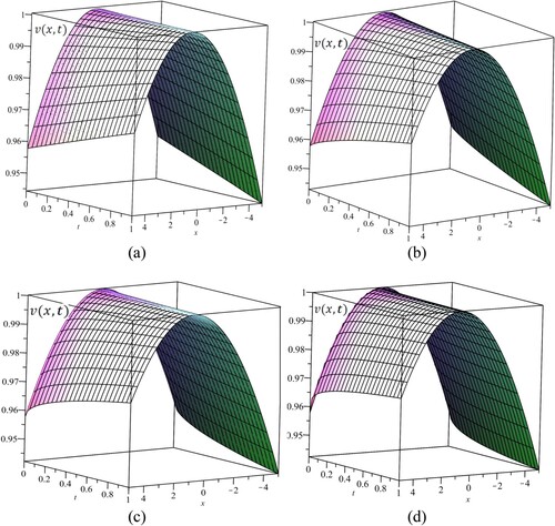
It is clear that for diverse values of the fractional-order α, the solution $u\left(x,t\right)$ remains a single soliton solution. This indicates the balancing script among the dispersion and nonlinearity remains true despite of the width and amplitude of the soliton are altered. The $\text{2D}$ and $\text{3D}$ figures appearing in Figure 2 outline the change of the structure of the soliton (width and amplitude) as a result of altering the fractional-order. This means that an increment in the fractional-order implies an increment in the altitude and the amplitude of the solitary wave solution. Figure 3 clarifies the effect of different values of the fractional-order on the amplitude of the soliton when x takes a certain value, say $x=0$. It is clear at a fixed value of the time $t$, the raise of the fractional-order implies a reducing the amplitude of the soliton wave solution.

Figure 2. (a) 3D graph and (b) 2D graph for $v\left(x,t\right)$ which relies only on x when the time $t=1$ for the fractional-order $\alpha$ with several values.

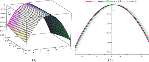
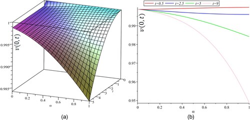
Figure 3. The distribution function amplitude for v(0; t) that depends only on the fractional-order $\alpha$ (a) 3D graph and (b) 2D graph.

Disclosure statement

No potential conflict of interest was reported by the author(s).

Correction Statement

This article has been republished with minor changes. These changes do not impact the academic content of the article.

Additional information

Funding

The authors acknowledge the Deanship of Scientific Research at King Faisal University for the financial support under Nasher Track [grant number 186034].

Appendix (He’s variational iteration method)

This method that has been developed by He (see, e.g. [52–57]) was utilized successfully to study wave equation that is either linear or nonlinear or wave-like equations in unbounded and bounded domains. Several researchers proved the reliability and efficiency of this method to be applicable to a large class of scientific applications to a large class of linear or nonlinear scientific applications (see, e.g. [58–61]). Furthermore, this method was proved sturdier than the current techniques, for instance, the Adomian method [62,63], perturbation method, etc. The method gives quickly convergent successive approximations of the exact solution in the case of its existence; or else, a few approximations can be utilized for numerical purposes. The computational procedures for the perturbation method are not an easy task, particularly, when the nonlinearity degree increases. Furthermore, the Adomian method possesses a difficult algorithm that is employed to find the Adomian polynomial that is required for nonlinear problems. While the present method does not demand specific requirements, such as small parameters, linearization and so on, for nonlinear operators. This method is considered an adjustment for the generic method of Lagrange multiplier [56,57]. It has been utilized successfully to construct the solution for integer nonlinear differential equations (see, e.g. [32,33]). In addition, it can be employed to build the solution fractional differential equations whether they are nonlinear or linear (see, e.g. [34–36]).

Consider the nonlinear partial differential equation (A1) $\hat{L}v\left(x,t\right)+\hat{N}v\left(x,t\right)=h\left(x,t\right),$(A1) where $\hat{L}$ and $\hat{N}$ represent the nonlinear and linear operator while h(x, t) acts the inhomogeneous term. Utilizing the iteration correction functional as [32,33], the $\left(n+1\right)\text{th}$ approximated solution for Equation (29) can be written as (A2) $\begin{array}{rl}{v}_{n+1}\left(x,t\right)& =v_n\left(x,t\right)+{\int }_0^t\lambda \left(\tau \right)\left[\hat{L}{v}_n\right(x,\tau )+\hat{N}{\tilde{v}}_n(x,\tau )\\ & -h\left(x,\tau \right)]\text{d}\tau ,n\ge 0,\end{array}$(A2) where λ(τ) represents the Lagrange multiplier that can be determined optimally by employing the variational theory while ${\tilde{v}}_n\left(x,t\right)$ is a restricted variation function, i.e. $\delta {\tilde{v}}_n\left(x,t\right)=0.$ The zeroth approximation $v_0\left(x,t\right)$ can be chosen as a solution of $\hat{L}v\left(x,t\right)=0$ or can be selected as the initial value $v\left(x,0\right)$. The exact solution for Equation (29) can be obtained when $n\to \mathrm{\infty },$ i.e. (A3) $v\left(x,t\right)=\underset{n\to \mathrm{\infty }}{lim}{v}_n\left(x,t\right).$(A3) Finally, we can summarize He’s variational method in the following algorithm:

Algorithm:

Step (1): Consider an equation in the form of Equation (29).

Step (2): Formulate Equation (30) which is considered the $\left(n+1\right)\text{th}$ approximated solution of Equation (29).

Step (3): Determine the Lagrange multiplier.

Step (4): Find the zeroth approximated solution, which can be taken as a solution for $\hat{L}v\left(x,t\right)=0$ or can be selected as an initial value.

Step (5): Insert the value of the Lagrange multiplier into Step (2) and find the approximated solutions for different values of $n$.

Step (6): For larger values of $n$, the approximated solution will be tended to the exact solution.

Step (7): Stop.

References

- Riewe F. Nonconservative Lagrangian and Hamiltonian mechanics. Phys Rev E. 1996;53:1890–1899. doi: 10.1103/PhysRevE.53.1890
- Riewe F. Mechanics with fractional derivatives. Phys Rev E. 1997;55:3581–3592. doi: 10.1103/PhysRevE.55.3581
- Agrawal OP. Formulation of Euler–Lagrange equations for fractional variational problems. J Math Anal Appl. 2002;272:368–379. doi: 10.1016/S0022-247X(02)00180-4
- Agrawal OP. Fractional variational calculus in terms of Riesz fractional derivatives. J Phys A Math Theor. 2007;40:6287. doi: 10.1088/1751-8113/40/24/003
- Attari M, Haeri M, Tavazoei MS. Analysis of a fractional order Van der Pol-like oscillator via describing function method. Nonlinear Dyn. 2010;61:265–274. doi: 10.1007/s11071-009-9647-0
- Tenreiro Machado JA. Calculation of fractional derivatives of noisy data with genetic algorithms. Non- Linear Dyn. 2009;57:253–260. doi: 10.1007/s11071-008-9436-1
- Mendes RV. A fractional calculus interpretation of the fractional volatility model. Nonlinear Dyn. 2009;55:395–399. doi: 10.1007/s11071-008-9372-0
- Frederico GSF, Torres DFM. Fractional conservation laws in optimal control theory. Nonlinear Dyn. 2008;53:215–222. doi: 10.1007/s11071-007-9309-z
- Baleanu D, Trujillo JI. A new method of finding the fractional Euler–Lagrange and Hamilton equations within Caputo fractional derivatives. Commun Nonlinear Sci Numer Simul. 2010;15:1111–1115. doi: 10.1016/j.cnsns.2009.05.023
- Yang XJ, Gao F, Srivastava HM. A new computational approach for solving nonlinear local fractional PDEs. J Comp Appl Math. 2018;339:285–296. doi: 10.1016/j.cam.2017.10.007
- Rui W. Applications of homogenous balanced principle on investigating exact solutions to a series of time fractional nonlinear PDEs. Comm Nonlin Sci Num Simul. 2017;47:253–266. doi: 10.1016/j.cnsns.2016.11.018
- Angstmann CN, Henry BI, Jacobs BA, et al. Integrablization of time fractional PDEs. Comput Math Appl. 2017;73:1053–1062. doi: 10.1016/j.camwa.2016.12.010
- Sakar MG, Uludag F, Erdogan F. Numerical solution of time-fractional nonlinear PDEs with proportional delays by homotopy perturbation method. Appl Math Model. 2016;40:6639–6649. doi: 10.1016/j.apm.2016.02.005
- Fernandez A, Baleanu D, Fokas AS. Solving PDEs of fractional order using the unified transform method. Appl Math Comp. 2018;339:738–749. doi: 10.1016/j.amc.2018.07.061
- Zhang S, Hong S. Variable separation method for a nonlinear time fractional partial differential equation with forcing term. J Comput Appl Math. 2018;339:297–305. doi: 10.1016/j.cam.2017.09.045
- Korteweg DJ, de Vries G. On the change of form of long waves advancing in a rectangular canal and on a new type of long stationary waves. Philos Mag. 1895;39:422–443. doi: 10.1080/14786449508620739
- Fung MK. Kdv equation as an Euler–Poincare’ equation. Chin J Phys. 1997;35:789–796.
- Elmandouha AA, Ibrahim AG. Bifurcation and travelling wave solutions for a (2+ 1)-dimensional KdV equation. J Taib Univ Sci. 2020;4:139–147. doi: 10.1080/16583655.2019.1709271
- Podlubny I. Fractional differential equations. San Diego (CA): Academic Press; 1999.
- Samko SG, Kilabas AA, Marichev OI. Fractional integrals and derivatives: theory and applications. New York: Gordon and Breach; 1998.
- Luchko Y, Srivastava HM. The exact solution of certain differential equations of fractional order by using operational calculus. Comput Math Appl. 1995;29:73–85. doi: 10.1016/0898-1221(95)00031-S
- Shah R, Li T. The thermal and laminar boundary layer flow over prolate and oblate spheroids. Int J Heat Mass Transfer. 2018;121:607–619. doi: 10.1016/j.ijheatmasstransfer.2017.12.130
- Arshad S, Sohail A, Maqbool K. Nonlinear shallow water waves: a fractional order approach. Alex Eng J. 2016;55:525–532. doi: 10.1016/j.aej.2015.10.014
- Ullah R, Ellahi R, Sait SM, et al. On the fractional-order model of HIV-1 infection of CD4+ T-cells under the influence of antiviral drug treatment. J Taib Univ Sci. 2020;14:50–59. doi: 10.1080/16583655.2019.1700676
- Sohail A, Maqbool K, Ellahi R. Stability analysis for fractional-order partial differential equations by means of space spectral time Adams-Bash forth Moulton method. Num Meth Part Diff Equat. 2018;34:19–29. doi: 10.1002/num.22171
- Khan U, Ellahi R, Khan R, et al. Extracting new solitary wave solutions of Benny–Luke equation and Phi-4 equation of fractional order by using (GI/G)-expansion method. Opt Quant Elect. 2017;49:362–376. doi: 10.1007/s11082-017-1191-4
- Ellahi R, Mohyud-Din ST, Khan U. Exact traveling wave solutions of fractional order Boussinesq-like equations by applying Exp-function method. Res. Phys. 2018;8:114–120.
- Babakhani A, Gejji VD. Existence of positive solutions of nonlinear fractional differential equations. J Math Anal Appl. 2003;278:434–442. doi: 10.1016/S0022-247X(02)00716-3
- Delbosco D. Fractional calculus and function spaces. J Fractal Calc. 1996;6:45–53.
- Zhang SQ. Existence of positive solution for some class of nonlinear fractional differential equations. J Math Anal Appl. 2003;278:136–148. doi: 10.1016/S0022-247X(02)00583-8
- Saha Ray S, Bera RK. An approximate solution of a nonlinear fractional differential equation by Adomian decomposition method. Appl Math Comput. 2005;167:561–571.
- He JH. A new approach to nonlinear partial differential equations. Commun Nonlinear Sci Numer Simul. 1997;2:230–235. doi: 10.1016/S1007-5704(97)90007-1
- He JH. Variational-iteration—a kind of nonlinear analytical technique: some examples. Int J Nonlinear Mech. 1999;34:699. doi: 10.1016/S0020-7462(98)00048-1
- He J-H. Approximate analytical solution for seepage flow with fractional derivatives in porous media. Comput Methods Appl Mech Eng. 1998;167:57–68. doi: 10.1016/S0045-7825(98)00108-X
- Momani S, Odibat Z, Alawnah A. Variational iteration method for solving the space- and time- fractional KdV equation. Numer Methods Part Differ Equat. 2008;24:261–271.
- Molliq RY, Noorani MSM, Hashim I. Variational iteration method for fractional heat- and wave-like equations. Nonlinear Anal Real World Appl. 2009;10:1854–1869. doi: 10.1016/j.nonrwa.2008.02.026
- Sohail A, Maqbool K, Hayat T. Painlevé property and approximate solutions using Adomian decom position for a nonlinear KdV-like wave equation. Appl Math Comput. 2014;229:359–366.
- Arqub OA, Maayah B. Fitted fractional reproducing kernel algorithm for the numerical solutions of ABC–fractional Volterra integro-differential equations. Chao Solit Fract. 2019;126:394–402. doi: 10.1016/j.chaos.2019.07.023
- Arqub OA, Maayah B. Modulation of reproducing kernel Hilbert space method for numerical solutions of Riccati and Bernoulli equations in the Atangana-Baleanu fractional sense. Chao Solit Fract. 2019;125:163–170. doi: 10.1016/j.chaos.2019.05.025
- Arqub OA, Al-Smadi M. An adaptive numerical approach for the solutions of fractional advection–diffusion and dispersion equations in singular case under Riesz’s derivative operator. Phys A Stat Mech Appl. 2020;540:123257. doi: 10.1016/j.physa.2019.123257
- Arqub OA. Application of residual power series method for the solution of time-fractional Schrodinger equations in one-dimensional space. Fund Inform. 2019;166:87–110. doi: 10.3233/FI-2019-1795
- Arqub OA. Numerical algorithm for the solutions of fractional order systems of Dirichlet function types with comparative analysis. Fund Inform. 2019;166:111–137. doi: 10.3233/FI-2019-1796
- El-Wakil SA, Abulwafa EM, Zahran MA, et al. Time-fractional KdV equation: formulation and solution using variational methods. Nonlinear Dyn. 2011;65:55–63. doi: 10.1007/s11071-010-9873-5
- Zhang Y. Formulation and solution to time-fractional generalized Korteweg-de Vries equation via variational methods. Adv Differ Equ. 2014;2014:65–77. doi: 10.1186/1687-1847-2014-65
- Khater AH, Moussa MHM, Abdul-Aziz SF. Invariant variational principles and conservation laws for some nonlinear partial differential equations with constant coefficients-II. Chaos Solitons Fractals. 2003;15:1–13. doi: 10.1016/S0960-0779(02)00059-0
- He JH. Semi-inverse method of establishing generalized variational principles for fluid mechanics with emphasis on turbo-machinery aerodynamics. Int J Turbo Jet-Engines. 1997;14:23–28.
- He JH. Variational principles for some nonlinear partial differential equations with variable coefficients. Chao Solit Fract. 2004;19:847–851. doi: 10.1016/S0960-0779(03)00265-0
- Kilbas AA, Srivastava HM, Trujillo JJ. Theory and applications of fractional differential equations. Amsterdam: Elsevier; 2006.
- Agrawal OP. A general formulation and solution scheme for fractional optimal control problems. Non- Linear Dyn. 2004;38:323–337. doi: 10.1007/s11071-004-3764-6
- Agrawal OP. Fractional variational calculus and the transversality conditions. J Phys A Math Gen. 2006;39:10375. doi: 10.1088/0305-4470/39/33/008
- He JH. Variational iteration method for autonomous ordinary differential systems. Appl Math Comput. 2000;114(2–3):115–123.
- He JH, Wu XH. Construction of solitary solution and compaction-like solution by variational iteration method. Chao Solit Fract. 2006;29:108–113. doi: 10.1016/j.chaos.2005.10.100
- He JH. A generalized variational principle in micromorphic thermoelasticity. Mech Res Comm. 2005;3291:93–98. doi: 10.1016/j.mechrescom.2004.06.006
- He JH. Variational iteration method—some recent results and new interpretations. J Comput Appl Math. 2007;207:3–17. doi: 10.1016/j.cam.2006.07.009
- Finlayson BA. The method of weighted residuals and variational principles. New York: Academic Press; 1972.
- Inokvti M, Sekine H, Mura T. General use of the Lagrange multiplier in nonlinear mathematical physics. In: Nemat-Nassed S, editor. Variational method in the mechanics of solids. U.S.A.: Pergamon Press; 1978. p. 156–162.
- Abulwafa EM, Abdou MA, Mahmoud AA. The solution of nonlinear coagulation problem with mass loss. Chao Solit Fract. 2006;29:313–330. doi: 10.1016/j.chaos.2005.08.044
- Momani S, Odibat Z. Analytical approach to linear fractional partial differential equations arising in fluid mechanics. Phys Lett A. 2006;1:1–9.
- Momani S, Abusaad S. Application of He’s variational-iteration method to Helmholtz equation. Chao Solit Fract. 2005;27:1119–1123. doi: 10.1016/j.chaos.2005.04.113
- Abdou MA, Soliman AA. Variational iteration method for solving Burgers’ and coupled Burgers’ equation. J Comput Appl Math. 2005;181:245–251. doi: 10.1016/j.cam.2004.11.032
- Adomian G. Solving Frontier problems of physics: the decomposition method. Boston (MA): Kluwer; 1994.
- Adomian G. A review of the decomposition method in applied mathematics. J Math Anal Appl. 1988;135:501–544. doi: 10.1016/0022-247X(88)90170-9