New methods to define heavy-tailed distributions with applications to insurance data

Abstract

Heavy-tailed distributions play an important role in modelling data in actuarial and financial sciences. In this article, nine new methods are suggested to define new distributions suitable for modelling data with an heavy right tail. For illustrative purposes, a special sub-model is considered in detail. Maximum likelihood estimators of the model parameters are obtained and a Monte Carlo simulation study is carried out to assess the behaviour of the estimators. Furthermore, some actuarial measures are calculated. A simulation study based on these actuarial measures is done. The usefulness of the proposed model is proved empirically by means of two real data sets. Finally, Bayesian analysis and performance of Gibbs sampling for the data sets are also carried out.

Keywords:

• Weibull distribution
• heavy-tailed distributions
• characterizations
• Monte Carlo simulation
• actuarial measures
• medical care insurance data
• vehicle insurance data
• Bayesian estimation

1. Introduction

In many applied areas, particularly in finance and actuarial sciences, data are usually positive, and their distribution is unimodal hump shaped and extreme values yield tails which are heavier than those of the standard well-known distributions. Classical distributions are not flexible enough to cater such heavy-tailed data sets. For example, (i) the Pareto distribution, which is widely used in modelling financial data sets, does not provide a reasonable fit for many applications and (ii) the Weibull model covers better the behaviour of small losses, but fails to cover the behaviour of large losses; see Bhati and Ravi [1]. In such situation, heavy-tailed distributions are reliable and accurate candidate models to employ. For positive data, heavy-tailed distributions are those whose right tail probabilities are greater than the exponential one (see Beirlant et al. [2]), that is $\underset{x\to \mathrm{\infty }}{lim}\frac{\exp \left(-\gamma x\right)}{1-F\left(x\right)}=0,\mathrm{f}\mathrm{o}\mathrm{r}\mathrm{a}\mathrm{n}\mathrm{y}\gamma >0,$ where $F\left(x\right)$ is the cumulative distribution function (cdf). For further detail, see McNeil [3] and Resnick [4]. Due to the importance of the heavy-tailed distributions in actuarial practice, the actuaries are motivated to introduce new flexible distributions. In this regard, serious attempts have been made and still growing rapidly. The new developments have been made through many different approaches such as (i) transformation of variables, (ii) composition of two or more distributions, (iii) compounding of distributions and (iv) finite mixture of distributions.

Recent studies of Eling [5] and Adcock et al. [6] identify that skew-normal and skew student t distributions are the best competitors as the skewed distributions adjust right-skewness and high kurtosis; for further detail see, Shushi [7] and Punzo [8]. However, insurance losses and financial risks take values on the positive real line and hence these skew class of distributions may not be appropriate as they are defined on $\mathbb{R}$. In such situations, the transformation of variables, particularly the exponential transformation, has proven to be substantial; see, for example, Azzalini et al. [9]. Bagnato and Punzo [10] showed that the transformation approach is simple to use but most often the inference as well as computation of the other distributional characteristics become complicated.

Another promising approach for obtaining new flexible heavy-tailed families of distributions, which gives reasonably good fit for heavy-tailed losses, is the method of composition; see Paula et al. [11], Klugman et al. [12], Nadarajah and Abu Bakar [13], and Bakar et al. [14]. However, it should be noted that the new distributions obtained by the composition approach involve more than three parameters causing difficulties in the estimation process and computational efforts are required.

Another prominent approach is compounding of distributions to cater data modelling with unimodality, right-skewness and heavy tails [8,15,16]. However, the density obtained via this method may not have a closed form expression which makes the estimation more cumbersome as shown in Punzo et al. [15]. For a brief review about compounding of distributions, we refer to Tahir and Cordeiro [17].

Finite mixture models represent a further approach to define very flexible distributions which are also able to capture, for instance, multimodality of the underlying distribution [18–20]. The price to pay for this greater flexibility is a more complicated and computationally challenging inference.

Furthermore, Dutta and Perry [21] performed an empirical analysis of loss distributions and risk was estimated by different approaches such as Exploratory Data Analysis and other empirical approaches. These authors rejected the idea of using the exponential, gamma and Weibull models in modelling insurance losses due to the poor results. They concluded that “one would need to use a model that is flexible enough in its structure”, and this encourages researchers to search for more flexible probability distributions providing greater accuracy in fitting heavy-tailed insurance losses.

Carrying out this branch of distribution theory, Alzaatreh et al. [22] defined the T-X family method to introduce new families of distributions. Let $v\left(t\right)$ be the probability density function (pdf) of a random variable, say T, where $T\in [m,n],$ $-\mathrm{\infty }\le m<n<\mathrm{\infty },$ and let $W\left[F\right(x\left)\right]$ be a function of $F\left(x\right)$ of a random variable, say X, satisfying the conditions given below:

1. $W\left[F\right(x\left)\right]\in [m,n]$,

2. $W\left[F\right(x\left)\right]$ is differentiable and monotonically increasing, and

3. $W\left[F\right(x\left)\right]\to m$ as $x\to -\mathrm{\infty }$ and $W\left[F\right(x\left)\right]\to n$ as $x\to \mathrm{\infty }$.

The cdf of the T-X family of distributions is defined by (1) $G\left(x\right)={\int }_m^{W\left[F\left(x\right)\right]}v\left(t\right)\mathrm{d}t,x\in \mathbb{R},$(1) where $W\left[F\right(x\left)\right]$ satisfies the conditions stated above. The pdf corresponding to (1(1) $G\left(x\right)={\int }_m^{W\left[F\left(x\right)\right]}v\left(t\right)\mathrm{d}t,x\in \mathbb{R},$(1) ) is $g\left(x\right)=\left\{\frac{\mathrm{\partial }}{\mathrm{\partial }x}W\left[F\left(x\right)\right]\right\}v\left\{W\left[F\left(x\right)\right]\right\},x\in \mathbb{R}.$ For the contributed work based on the idea of T-X approach, we refer to Ahmad et al. [23]. Using the approach of T-X method, one can introduce new members of survival family [24] via the cdf (2) $G\left(x\right)=1-{\int }_m^{W\left[\overline{F}\left(x\right)\right]}v\left(t\right)\mathrm{d}t,x\in \mathbb{R},$(2) where $\overline{F}\left(x\right)=1-F\left(x\right)$ is the survival function of the baseline distribution.

Recently, Mahdavi and Kundu [25] proposed a new prominent approach for introducing statistical distributions via the cdf given by (3) $G\left(x;\alpha ,\xi \right)=\frac{{\alpha }^{F\left(x;\xi \right)}-1}{\alpha -1},\alpha >1,\alpha \ne 1,x\in \mathbb{R}$(3) with additional parameter α.

Under these premises, we are motivated to propose new families of distributions. Taking inspiration from (1(1) $G\left(x\right)={\int }_m^{W\left[F\left(x\right)\right]}v\left(t\right)\mathrm{d}t,x\in \mathbb{R},$(1) )–(3(3) $G\left(x;\alpha ,\xi \right)=\frac{{\alpha }^{F\left(x;\xi \right)}-1}{\alpha -1},\alpha >1,\alpha \ne 1,x\in \mathbb{R}$(3) ), in this article, nine new families of distributions are proposed.

The paper is outlined as follows: new development to the heavy-tailed distributions is presented in Section 2. In Section 3, we define a special sub-model of the proposed family and provide plots of the density function. We derive some statistical properties in Section 4. Some characterizations results are provided in Section 5. Maximum likelihood estimation of the model parameters is addressed in Section 6. In the same section, the Monte Carlo simulation study is provided. Actuarial measures of the proposed method along with a simulation study are provided in Section 7. In Section 8, we provide two applications to real data to illustrate the importance of the new family. Bayesian analysis as well as a Gibbs sampling procedure for the considered data sets are discussed in Section 9. Finally, some concluding remarks are presented in Section 10.

2. New contribution to heavy-tailed distributions

As we mentioned in Section 1, the researchers are often in search of new heavy-tailed distributions suitable for modelling insurance losses. In this section, we propose some new useful methods to obtain heavy-tailed extended versions of the existing distributions.

2.1. New extended exponentiated-X family

Taking inspiration from (1(1) $G\left(x\right)={\int }_m^{W\left[F\left(x\right)\right]}v\left(t\right)\mathrm{d}t,x\in \mathbb{R},$(1) ), we introduce a new flexible class of distributions. The proposed class is called a new extended exponentiated-X (NEEx-X) family. Let T ∼ exp(1), then its cdf is given by (4) $V\left(t\right)=1-e^{-t},t\ge 0.$(4) The density function corresponding to (4(4) $V\left(t\right)=1-e^{-t},t\ge 0.$(4) ) is (5) $v\left(t\right)=e^{-t},t>0.$(5) If $v\left(t\right)$ follows (5(5) $v\left(t\right)=e^{-t},t>0.$(5) ) and setting $W\left[F\right(x\left)\right]=-\log \left\{\frac{1-\theta F{\left(x;\xi \right)}^a}{1-\log \left[1-F{\left(x;\xi \right)}^a\right]}\right\}$ in (1(1) $G\left(x\right)={\int }_m^{W\left[F\left(x\right)\right]}v\left(t\right)\mathrm{d}t,x\in \mathbb{R},$(1) ), we define the cdf of the NEEx-X family given by (6) $G\left(x\right)=1-\frac{1-\theta F{\left(x;\xi \right)}^a}{1-\log \left[1-F{\left(x;\xi \right)}^a\right]},a,\theta >0,x\in \mathbb{R},$(6) where $F(x;\xi )$ is the cdf of the baseline distribution depending on the parameter $\xi \in \mathbb{R}$. The pdf of the NEEx-X family is $\begin{array}{rl}g\left(x\right)& =\frac{af\left(x;\xi \right)F{\left(x;\xi \right)}^{a-1}}{{\left\{1-\log \left[A\left(x\right)\right]\right\}}^2}\\ & \times \left\{\theta \left\{1-\log \left[A\left(x\right)\right]\right\}+\frac{1-\theta F{\left(x;\xi \right)}^a}{A\left(x\right)}\right\},\\ & x\in \mathbb{R},\end{array}$ where $A\left(x\right)=1-F(x;\xi {)}^a$. For a = 1, the NEEx-X family gives the new extended-X(NE-X) family.

2.2. New type-I cosine exponentiated-X family

Again taking inspiration from (1(1) $G\left(x\right)={\int }_m^{W\left[F\left(x\right)\right]}v\left(t\right)\mathrm{d}t,x\in \mathbb{R},$(1) ), we introduce another new family of distributions, called new type-I cosine exponentiated-X(NTICEx-X) family. If $v\left(t\right)$ follows (5(5) $v\left(t\right)=e^{-t},t>0.$(5) ) and setting $W\left[F\right(x\left)\right]=-\log \left\{\frac{\cos \left(\frac{\pi }{2}F(x;\xi {)}^a\right]}{1-\log [1-F(x;\xi {)}^a]}\right\}$ in (1(1) $G\left(x\right)={\int }_m^{W\left[F\left(x\right)\right]}v\left(t\right)\mathrm{d}t,x\in \mathbb{R},$(1) ), we define the cdf of the NTICEx-X family via (7) $G\left(x\right)=1-\frac{\cos \left[\frac{\pi }{2}F{\left(x;\xi \right)}^a\right]}{1-\log \left[1-F{\left(x;\xi \right)}^a\right]},a>0,x\in \mathbb{R},$(7) with pdf $\begin{array}{rl}g\left(x\right)& =\frac{af\left(x;\xi \right)F{\left(x;\xi \right)}^{a-1}}{{\left\{1-\log \left[A\left(x\right)\right]\right\}}^2}\left\{\phantom{\frac{\cos \left(\frac{\pi }{2}F{\left(x;\xi \right)}^a\right)}{A\left(x\right)}}\frac{\pi }{2}\left\{1-\log \left[A\left(x\right)\right]\right\}\right.\\ & \times \left.\sin \left(\frac{\pi }{2}F{\left(x;\xi \right)}^a\right)+\frac{\cos \left(\frac{\pi }{2}F{\left(x;\xi \right)}^a\right)}{A\left(x\right)}\right\},\\ & x\in \mathbb{R}.\end{array}$ For $a=1,$ the NTICEx-X family gives the new type-I cosine-X(NTIC-X) family.

2.3. Type-I cosine exponentiated-X family

Taking inspiration from (2(2) $G\left(x\right)=1-{\int }_m^{W\left[\overline{F}\left(x\right)\right]}v\left(t\right)\mathrm{d}t,x\in \mathbb{R},$(2) ), we introduce a new method of proposing distributions. The proposed method is called type-I cosine exponentiated-X(TICEx-X) family of distributions. If $v\left(t\right)$ follows (5(5) $v\left(t\right)=e^{-t},t>0.$(5) ) and setting $W\left[\overline{F}\right(x\left)\right]=-\log \left\{\frac{\cos \left(\frac{\pi }{2}[1-F(x;\xi {)}^a]\right)}{1-\log [1-F(x;\xi {)}^a]}\right\}$ in (2(2) $G\left(x\right)=1-{\int }_m^{W\left[\overline{F}\left(x\right)\right]}v\left(t\right)\mathrm{d}t,x\in \mathbb{R},$(2) ), we define the cdf of the TICEx-X family given by (8) $G\left(x\right)=\frac{\cos \left[\frac{\pi }{2}\left\{1-F{\left(x;\xi \right)}^a\right\}\right]}{1-\log \left[1-F{\left(x;\xi \right)}^a\right]},a>0,x\in \mathbb{R}.$(8) The density function corresponding to (8(8) $G\left(x\right)=\frac{\cos \left[\frac{\pi }{2}\left\{1-F{\left(x;\xi \right)}^a\right\}\right]}{1-\log \left[1-F{\left(x;\xi \right)}^a\right]},a>0,x\in \mathbb{R}.$(8) ) is $\begin{array}{rl}g\left(x\right)& =\frac{af\left(x;\xi \right)F{\left(x;\xi \right)}^{a-1}}{{\left(1-\log \left[A\left(x\right)\right]\right)}^2}\left\{\phantom{\frac{\cos \left(\frac{\pi }{2}A\left(x\right)\right)}{A\left(x\right)}}\frac{\pi }{2}\sin \left(\frac{\pi }{2}A\left(x\right)\right)\right.\\ & \times \left.\left(1-\log \left[A\left(x\right)\right]\right)-\frac{\cos \left(\frac{\pi }{2}A\left(x\right)\right)}{A\left(x\right)}\right\},\\ & a>0,x\in \mathbb{R}.\end{array}$ For a = 1, the TICEx-X family gives the new Type-I cosine-X (TIC-X) family.

2.4. The exponent power exponentiated-X family

Take inspiration from (3(3) $G\left(x;\alpha ,\xi \right)=\frac{{\alpha }^{F\left(x;\xi \right)}-1}{\alpha -1},\alpha >1,\alpha \ne 1,x\in \mathbb{R}$(3) ), we introduce a new method of proposing probability distributions, called the exponent power exponentiated-X (EPEx-X) family of distributions. The cdf of the EPEx-X family is defined by the following expression (9) $G\left(x\right)=\frac{e^{\left\{1-\frac{\theta }{\theta -\log \left[1-F{\left(x;\xi \right)}^a\right]}\right\}}-1}{e-1},a,\theta >0,x\in \mathbb{R}.$(9) The pdf corresponding to (9(9) $G\left(x\right)=\frac{e^{\left\{1-\frac{\theta }{\theta -\log \left[1-F{\left(x;\xi \right)}^a\right]}\right\}}-1}{e-1},a,\theta >0,x\in \mathbb{R}.$(9) ) is $\begin{array}{rl}g\left(x\right)& =\frac{a\theta f\left(x;\xi \right)F{\left(x;\xi \right)}^{a-1}{e}^{\left\{1-\frac{\theta }{\theta -\log \left[1-F{\left(x;\xi \right)}^a\right]}\right\}}}{\left(e-1\right)\left[1-F{\left(x;\xi \right)}^a\right]{\left\{\theta -\log \left[1-F{\left(x;\xi \right)}^a\right]\right\}}^2},\\ & x\in \mathbb{R}.\end{array}$ For $a=1,$ in (9(9) $G\left(x\right)=\frac{e^{\left\{1-\frac{\theta }{\theta -\log \left[1-F{\left(x;\xi \right)}^a\right]}\right\}}-1}{e-1},a,\theta >0,x\in \mathbb{R}.$(9) ), we introduce a sub-case of the EPEx-X family, called the exponent power-X (EP-X) family by cdf (10) $G\left(x\right)=\frac{e^{\left\{1-\frac{\theta }{\theta -\log \left[1-F\left(x;\xi \right)\right]}\right\}}-1}{e-1},\theta >0,x\in \mathbb{R}.$(10) The pdf corresponding to (10(10) $G\left(x\right)=\frac{e^{\left\{1-\frac{\theta }{\theta -\log \left[1-F\left(x;\xi \right)\right]}\right\}}-1}{e-1},\theta >0,x\in \mathbb{R}.$(10) ) is (11) $\begin{array}{rl}g\left(x\right)& =\frac{\theta f\left(x;\xi \right)e^{\left\{1-\frac{\theta }{\theta -\log \left[1-F\left(x;\xi \right)\right]}\right\}}}{\left(e-1\right)\left[1-F\left(x;\xi \right)\right]{\left\{\theta -\log \left[1-F\left(x;\xi \right)\right]\right\}}^2},\\ & x\in \mathbb{R}.\end{array}$(11) For $\theta =1,$ the EP-X family gives the new reduced exponent power-X (REP-X) family.

3. The exponent power-Weibull distribution: a new heavy-tailed distribution

In this section, we define a special sub-model of the exponent power-X family, called exponent power-Weibull (EP-W) distribution. Let $F\left(x;\xi \right)$ be the cdf of the Weibull distribution given by $F(x;\xi )=1-e^{-\gamma x^{\alpha }},x\ge 0$, where $\xi =\left(\alpha ,\gamma \right)$. Then, the cdf of the EP-W distribution has the following expression (12) $G\left(x;\theta ,\xi \right)=\frac{e^{\left(\frac{\gamma x^{\alpha }}{\theta +\gamma x^{\alpha }}\right)}-1}{e-1},x\ge 0,\alpha ,\theta ,\gamma >0.$(12) The pdf corresponding to (12(12) $G\left(x;\theta ,\xi \right)=\frac{e^{\left(\frac{\gamma x^{\alpha }}{\theta +\gamma x^{\alpha }}\right)}-1}{e-1},x\ge 0,\alpha ,\theta ,\gamma >0.$(12) ) is given by (13) $g\left(x;\theta ,\xi \right)=\frac{\alpha \theta \gamma x^{\alpha -1}}{\left(e-1\right){\left(\theta +\gamma x^{\alpha }\right)}^2}{e}^{\left(\frac{\gamma x^{\alpha }}{\theta +\gamma x^{\alpha }}\right)},x>0.$(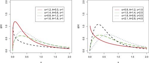13) Some possible shapes for the pdf of the EP-W distribution, for selected values of the model parameters, are sketched in Figure 1.

Figure 1. Different plots for the pdf of the EP-W distribution.

4. Statistical properties

In this section, we study some statistical properties of the EP-W distribution such as quantile function, moments and moment generating function (mgf). Some key advantages of the EP-W distribution are:

• The mean and variance of the distribution are in explicit forms and simple to calculate.

• The quantile function of the distribution has a closed form which makes it easier to generate random numbers.

4.1. Quantile function

Let X be the random variable follow the EP-W distribution with cdf (12(12) $G\left(x;\theta ,\xi \right)=\frac{e^{\left(\frac{\gamma x^{\alpha }}{\theta +\gamma x^{\alpha }}\right)}-1}{e-1},x\ge 0,\alpha ,\theta ,\gamma >0.$(12) ). Then, the quantile function (qf) of X, say $x_u=Q\left(u\right)=G^{-1}\left(u\right)$, can be obtained by inverting (12(12) $G\left(x;\theta ,\xi \right)=\frac{e^{\left(\frac{\gamma x^{\alpha }}{\theta +\gamma x^{\alpha }}\right)}-1}{e-1},x\ge 0,\alpha ,\theta ,\gamma >0.$(12) ) as follows (14) $x_u=Q\left(u\right)={\left\{\left(\frac{\gamma }{\theta }{\left[\log \left(u\left(e-1\right)+1\right)\right]}^{-1}-1\right)\right\}}^{-\frac{1}{\alpha }},$(14) where u ∈ (0,1). The qf of the EP-W distribution has a closed form expression. In particular, the first quartile, second quartile (median) and third quartile are obtained by substituting $u=$ 0.25, 0.5 and 0.75 in (14(14) $x_u=Q\left(u\right)={\left\{\left(\frac{\gamma }{\theta }{\left[\log \left(u\left(e-1\right)+1\right)\right]}^{-1}-1\right)\right\}}^{-\frac{1}{\alpha }},$(14) ), respectively.

4.2. Moments

Some of the most important features and characteristics of a model can be obtain through its moments. The rth moment of a random variable X, say ${\mu }_r^{/}$, with pdf (13(13) $g\left(x;\theta ,\xi \right)=\frac{\alpha \theta \gamma x^{\alpha -1}}{\left(e-1\right){\left(\theta +\gamma x^{\alpha }\right)}^2}{e}^{\left(\frac{\gamma x^{\alpha }}{\theta +\gamma x^{\alpha }}\right)},x>0.$(13) ) is derived as (15) ${\mu }_r^{/}={\int }_0^{\mathrm{\infty }}\frac{\alpha \theta \gamma x^{\alpha +r-1}}{\left(e-1\right){\left(\theta +\gamma x^{\alpha }\right)}^2}{e}^{\left(\frac{\gamma x^{\alpha }}{\theta +\gamma x^{\alpha }}\right)}\mathrm{d}x.$(15) On solving, we have ${\mu }_r^{/}=\sum _{i=0}^{\mathrm{\infty }}\frac{1}{{\eta }^{\frac{r}{\alpha }}\left(e-1\right)i!}{\int }_0^{\mathrm{\infty }}\frac{t^{\left(\frac{r}{\alpha }+i+1\right)-1}}{{\left(1+t\right)}^{\left(\frac{r}{\alpha }+i+1\right)+\left(\frac{\alpha -r}{\alpha }\right)}}\mathrm{d}t,$ where $\eta =\gamma /\theta$. Using the definition of Beta type-II distribution, we have (16) ${\mu }_r^{/}=\sum _{i=0}^{\mathrm{\infty }}\frac{B\left(\left(\frac{r}{\alpha }+i+1\right),\left(\frac{\alpha -r}{\alpha }\right)\right)}{{\eta }^{\frac{r}{\alpha }}\left(e-1\right)i!}.$(16) For r = 1, in (16(16) ${\mu }_r^{/}=\sum _{i=0}^{\mathrm{\infty }}\frac{B\left(\left(\frac{r}{\alpha }+i+1\right),\left(\frac{\alpha -r}{\alpha }\right)\right)}{{\eta }^{\frac{r}{\alpha }}\left(e-1\right)i!}.$(16) ), we get the first raw moment (mean) of the EP-W distribution given by (17) ${\mu }_1^{/}=\sum _{i=0}^{\mathrm{\infty }}\frac{B\left(\left(\frac{1}{\alpha }+i+1\right),\left(\frac{\alpha -1}{\alpha }\right)\right)}{{\eta }^{\frac{1}{\alpha }}\left(e-1\right)i!}.$(17) Similarly, the second raw moment of the EP-W distribution is given by (18) ${\mu }_2^{/}=\sum _{i=0}^{\mathrm{\infty }}\frac{B\left(\left(\frac{2}{\alpha }+i+1\right),\left(\frac{\alpha -2}{\alpha }\right)\right)}{{\eta }^{\frac{2}{\alpha }}\left(e-1\right)i!}.$(18) Now, the variance of the proposed distribution is obtained by using the following relation (19) ${\mu }_2={\mu }_2^{/}-{\left({\mu }_1^{/}\right)}^2.$(19) Using (17(17) ${\mu }_1^{/}=\sum _{i=0}^{\mathrm{\infty }}\frac{B\left(\left(\frac{1}{\alpha }+i+1\right),\left(\frac{\alpha -1}{\alpha }\right)\right)}{{\eta }^{\frac{1}{\alpha }}\left(e-1\right)i!}.$(17) ) and (18(18) ${\mu }_2^{/}=\sum _{i=0}^{\mathrm{\infty }}\frac{B\left(\left(\frac{2}{\alpha }+i+1\right),\left(\frac{\alpha -2}{\alpha }\right)\right)}{{\eta }^{\frac{2}{\alpha }}\left(e-1\right)i!}.$(18) ) in (19(19) ${\mu }_2={\mu }_2^{/}-{\left({\mu }_1^{/}\right)}^2.$(19) ), we obtain the variance of the EP-W distribution. Furthermore, the mgf of the EP-W distribution, $M_X\left(t\right)$, is given by $\begin{array}{rl}{M}_X\left(t\right)& =\sum _{r,i=0}^{\mathrm{\infty }}\frac{t^r}{{\eta }^{\frac{r}{\alpha }}\left(e-1\right)i!r!}\\ & \times B\left(\left(\frac{r}{\alpha }+i+1\right),\left(\frac{\alpha -r}{\alpha }\right)\right).\end{array}$ The graphs of skewness and kurtosis of the EP-W distribution along with the corresponding contour plots are presented in Figures 2 and 3, respectively.

Figure 2. Skewness and the corresponding contour plot of the EP-W distribution.

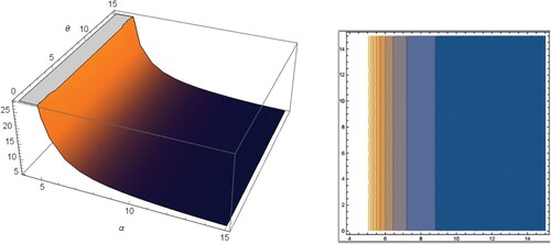
Figure 3. Kurtosis and the corresponding contour plot of the EP-W distribution.

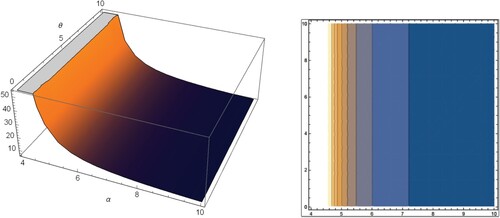
From Figures 2 and 3, it is clear that for fixed values of θ, the skewness is decreased when α is increased. (ii) For fixed values of α, the skewness is increased when θ is increased. (iii) For fixed values of θ, the kurtosis is decreased when α is increased.

5. Characterization results

In designing a stochastic model for a particular data set, an investigator will be vitally interested to know if their selected model fits the necessary requirements. To this end, the investigator will rely on the characterizations of the selected distribution. Thus, the problem of characterizing a distribution is important in various fields and has recently attracted the attention of many researchers. Consequently, various characterization results have been reported in the literature. These characterizations have been established in different directions. This section is devoted to certain characterizations of the EP-X distribution based on a simple relationship between two truncated moments. Due to the nature of the cdf of this distribution, our characterizations may be the only possible ones. The first characterization result employs Theorem 1 of Glänzel [26], given in Appendix. As shown in Glänzel [27], this characterization is stable in the sense of weak convergence and can also be employed when the cdf does not have a closed form. We would like to mention that the goal of Theorem A.1 is to make $\eta \left(x\right)$ as simple as possible.

Proposition 5.1

Suppose X is a continuous random variable. Let $q_1\left(x\right)=\exp \left\{\frac{\theta }{\theta -\log (1-F(x;\xi \left)\right)}-1\right\}$ and $q_2\left(x\right)=q_1\left(x\right)\{\theta -\log (1-F(x;\xi )){\}}^{-1}$ for $x\in \mathbb{R}$. Then X has density function (11(11) $\begin{array}{rl}g\left(x\right)& =\frac{\theta f\left(x;\xi \right)e^{\left\{1-\frac{\theta }{\theta -\log \left[1-F\left(x;\xi \right)\right]}\right\}}}{\left(e-1\right)\left[1-F\left(x;\xi \right)\right]{\left\{\theta -\log \left[1-F\left(x;\xi \right)\right]\right\}}^2},\\ & x\in \mathbb{R}.\end{array}$(11) ) if and only if the function η, defined in Theorem A.1, is given by $\eta \left(x\right)=\frac{1}{2}{\left\{\theta -\log \left(1-F\left(x;\xi \right)\right)\right\}}^{-1},x\in \mathbb{R}.$

Proof.

Suppose X is a random variable with density function (11(11) $\begin{array}{rl}g\left(x\right)& =\frac{\theta f\left(x;\xi \right)e^{\left\{1-\frac{\theta }{\theta -\log \left[1-F\left(x;\xi \right)\right]}\right\}}}{\left(e-1\right)\left[1-F\left(x;\xi \right)\right]{\left\{\theta -\log \left[1-F\left(x;\xi \right)\right]\right\}}^2},\\ & x\in \mathbb{R}.\end{array}$(11) ), then we have $\begin{array}{rl}& \left(1-G\left(x\right)\right)E\left[q_1\left(X\right)|X\ge x\right]\\ & =\frac{\theta }{e-1}{\left\{\theta -\log \left(1-F\left(x;\xi \right)\right)\right\}}^{-1},x\in \mathbb{R},\\ & \left(1-G\left(x\right)\right)E\left[q_2\left(X\right)|X\ge x\right]\\ & =\frac{\theta }{2\left(e-1\right)}{\left\{\theta -\log \left(1-F\left(x;\xi \right)\right)\right\}}^{-2},x\in \mathbb{R},\end{array}$ and $\begin{array}{rl}& \eta \left(x\right)q_1\left(x\right)-q_2\left(x\right)\\ & =-\frac{1}{2}{q}_1\left(x\right){\left\{\theta -\log \left(1-F\left(x;\xi \right)\right)\right\}}^{-1}<0\\ & \mathrm{f}\mathrm{o}\mathrm{r}x\in \mathbb{R}.\end{array}$ Conversely, if η is of the above form, then $\begin{array}{rl}{s}^{\mathrm{\prime }}\left(x\right)& =\frac{{\eta }^{\mathrm{\prime }}\left(x\right)q_1\left(x\right)}{\eta \left(x\right)q_1\left(x\right)-q_2\left(x\right)}\\ & =\frac{f\left(x;\xi \right){\left\{\theta -\log \left(1-F\left(x;\xi \right)\right)\right\}}^{-1}}{1-F\left(x;\xi \right)},x\in \mathbb{R},\end{array}$ and consequently $s\left(x\right)=\log \left(\left\{\theta -\log \left(1-F\left(x;\xi \right)\right)\right\}\right),x\in \mathbb{R}.$ Now, according to Theorem A.1, X has pdf (11(11) $\begin{array}{rl}g\left(x\right)& =\frac{\theta f\left(x;\xi \right)e^{\left\{1-\frac{\theta }{\theta -\log \left[1-F\left(x;\xi \right)\right]}\right\}}}{\left(e-1\right)\left[1-F\left(x;\xi \right)\right]{\left\{\theta -\log \left[1-F\left(x;\xi \right)\right]\right\}}^2},\\ & x\in \mathbb{R}.\end{array}$(11) ).

Corollary 5.1

Suppose $X:\mathrm{\Omega }\to \mathbb{R}$ is a continuous random variable and $q_1\left(x\right)$ is as in Proposition 5.1. Then X has density function (11(11) $\begin{array}{rl}g\left(x\right)& =\frac{\theta f\left(x;\xi \right)e^{\left\{1-\frac{\theta }{\theta -\log \left[1-F\left(x;\xi \right)\right]}\right\}}}{\left(e-1\right)\left[1-F\left(x;\xi \right)\right]{\left\{\theta -\log \left[1-F\left(x;\xi \right)\right]\right\}}^2},\\ & x\in \mathbb{R}.\end{array}$(11) ) if and only if there exist functions $q_2$ and η defined in Theorem A.1 satisfying the following first-order differential equation $\begin{array}{rl}\frac{{\eta }^{\mathrm{\prime }}\left(x\right)q_1\left(x\right)}{\eta \left(x\right)q_1\left(x\right)-q_2\left(x\right)}& =\frac{f\left(x;\xi \right){\left\{\theta -\log \left(1-F\left(x;\xi \right)\right)\right\}}^{-1}}{1-F\left(x;\xi \right)},\\ & x\in \mathbb{R}.\end{array}$

Corollary 5.2

The differential equation in Corollary 5.1 has the following general solution (20) $\begin{array}{rl}\eta \left(x\right)& ={\left\{\theta -\log \left(1-F\left(x;\xi \right)\right)\right\}}^{-1}\\ & \times \left[\int \frac{f\left(x;\xi \right)}{1-F\left(x;\xi \right)}{\left(q_1\left(x\right)\right)}^{-1}{q}_2\left(x\right)\mathrm{d}x+D\right],\end{array}$(20) in which D is a constant. We like to mention that a set of functions satisfying the above first-order differential equation is given in Proposition 5.1 with $D=0.$ Clearly, there are other triplets $(q_1,q_2,\eta )$ satisfying the conditions of Theorem A.1.

6. Maximum likelihood estimation and Monte Carlo simulation study

In this section, we use the maximum likelihood method to estimate model parameters and also provide a Monte Carlo simulations to assess the behaviour of these estimators.

6.1. Maximum likelihood estimation

In this sub-section, we obtain the maximum likelihood estimators (MLEs) of the model parameters of the EP-W distribution from complete samples only. Let $x_1,x_2,,x_n$ be an observed sample of size n obtained from (13(13) $g\left(x;\theta ,\xi \right)=\frac{\alpha \theta \gamma x^{\alpha -1}}{\left(e-1\right){\left(\theta +\gamma x^{\alpha }\right)}^2}{e}^{\left(\frac{\gamma x^{\alpha }}{\theta +\gamma x^{\alpha }}\right)},x>0.$(13) ). The corresponding log-likelihood function can be expressed as (21) $\begin{array}{rl}\log L\left(x;\alpha ,\theta ,\gamma \right)& =-n\log \left(e-1\right)+n\log \left(\alpha \right)+n\log \left(\theta \right)\\ & +n\log \left(\gamma \right)+\left(\alpha -1\right)\sum _{i=1}^n\log \left(x_i\right)\\ & -2\sum _{i=1}^n\log \left(\theta +\gamma x_i^{\alpha }\right)+\sum _{i=1}^n\frac{\gamma x_i^{\alpha }}{\theta +\gamma x_i^{\alpha }}.\end{array}$(21) The partial derivatives of (21(21) $\begin{array}{rl}\log L\left(x;\alpha ,\theta ,\gamma \right)& =-n\log \left(e-1\right)+n\log \left(\alpha \right)+n\log \left(\theta \right)\\ & +n\log \left(\gamma \right)+\left(\alpha -1\right)\sum _{i=1}^n\log \left(x_i\right)\\ & -2\sum _{i=1}^n\log \left(\theta +\gamma x_i^{\alpha }\right)+\sum _{i=1}^n\frac{\gamma x_i^{\alpha }}{\theta +\gamma x_i^{\alpha }}.\end{array}$(21) ) with respect to the parameters $\left(\alpha ,\theta ,\gamma \right)$ are given, respectively, by (22) $\begin{array}{rl}\frac{\mathrm{\partial }\log L\left(x;\alpha ,\theta ,\gamma \right)}{\mathrm{\partial }\alpha }& =\frac{n}{\alpha }+\sum _{i=1}^n\log \left(x_i\right)\\ & +\sum _{i=1}^n\frac{\begin{array}{c}\gamma x_i^{\alpha }\left(\log x_i\right)\\ \left\{\left(\theta +\gamma x_i^{\alpha }\right)-x_i^{\alpha }\right\}\end{array}}{{\left(\theta +\gamma x_i^{\alpha }\right)}^2}\\ & -2\gamma \sum _{i=1}^n\frac{\left(\log x_i\right)x_i^{\alpha }}{\left(\theta +\gamma x_i^{\alpha }\right)},\end{array}$(22) (23) $\begin{array}{rl}\frac{\mathrm{\partial }\log L\left(x;\alpha ,\theta ,\gamma \right)}{\mathrm{\partial }\theta }& =\frac{n}{\theta }-2\sum _{i=1}^n\frac{1}{\left(\theta +\gamma x_i^{\alpha }\right)}\\ & -\sum _{i=1}^n\frac{\gamma x_i^{\alpha }}{{\left(\theta +\gamma x_i^{\alpha }\right)}^2},\end{array}$(23) and (24) $\begin{array}{rl}\frac{\mathrm{\partial }\log L\left(x;\alpha ,\theta ,\gamma \right)}{\mathrm{\partial }\gamma }& =\frac{n}{\gamma }-2\sum _{i=1}^n\frac{x_i^{\alpha }}{\left(\theta +\gamma x_i^{\alpha }\right)}\\ & +\sum _{i=1}^n\frac{\theta x_i^{\alpha }}{{\left(\theta +\gamma x_i^{\alpha }\right)}^2}.\end{array}$(24) Solving $\begin{array}{rl}& \frac{\mathrm{\partial }\log L\left(x;\alpha ,\theta ,\gamma \right)}{\mathrm{\partial }\alpha }=0,\\ & \frac{\mathrm{\partial }\log L\left(x;\alpha ,\theta ,\gamma \right)}{\mathrm{\partial }\theta }=0\mathrm{a}\mathrm{n}\mathrm{d}\\ & \frac{\mathrm{\partial }\log L\left(x;\alpha ,\theta ,\gamma \right)}{\mathrm{\partial }\gamma }=0,\end{array}$ simultaneously yields the MLEs $\left(\hat{\alpha },\hat{\theta },\hat{\gamma }\right)$ of $\left(\alpha ,\theta ,\gamma \right).$

6.2. Monte Carlo simulation study

In this sub-section, we perform a Monte Carlo (MC) simulation study with the objective to assess the behaviour of the MLEs of EP-W model via the optim()R-function with the argument method = "L-BFGS-B"; see Appendix. It is used for maximizing the log-likelihood function of a probabilistic model. We consider 750 MC-replicates under different sample sizes $n=25,50,\dots ,750$. For each sample size, we compute the average MLEs, mean square errors (MSE), Biases and Absolute biases. The results obtained after performing the MC simulation are provided in Table 1 and displayed graphically in Figures 4–7.

Figure 4. Plots of MLEs and MSEs of the EP-W model for $\alpha =1.4$, $\theta =0.5$ and $\gamma =1$.

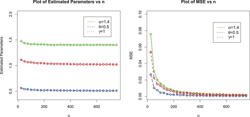
Figure 5. Plots of Biases and absolute biases of the EP-W model for $\alpha =1.4$, $\theta =0.5$ and $\gamma =1$.

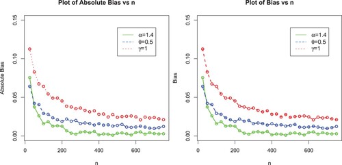
Figure 6. Plots of MLEs and MSEs of the EP-W model for $\alpha =1.6$, $\theta =1.2$ and $\gamma =1$.

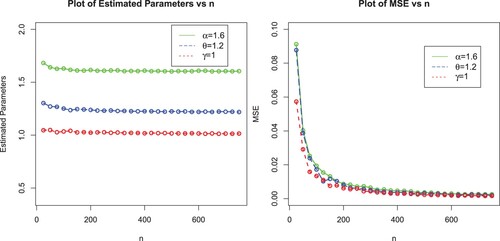
Figure 7. Plots of biases and absolute biases of the EP-W model for $\alpha =1.6$, $\theta =1.2$ and $\gamma =1$.

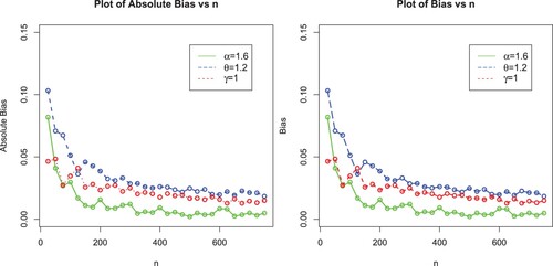
Table 1. Simulation results for the EP-W distribution.

		Set 1: $\alpha =1.4$, $\theta =0.5$, $\gamma =1$			Set 2: $\alpha =1.6$, $\theta =1.2$, $\gamma =1$
n	parameters	MLE	MSEs	Biases	MLE	MSEs	Biases
25	$\hat{\alpha }$	1.45781	0.07176	0.05781	1.68430	0.09778	0.08430
	$\hat{\theta }$	0.56975	0.03086	0.06975	1.29588	0.08168	0.09588
	$\hat{\gamma }$	1.11005	0.05338	0.11005	1.06545	0.07545	0.06545
50	$\hat{\alpha }$	1.44211	0.03493	0.04211	1.64965	0.04159	0.04965
	$\hat{\theta }$	0.54253	0.01148	0.04253	1.27387	0.03730	0.07387
	$\hat{\gamma }$	1.09308	0.02794	0.09308	1.03817	0.02547	0.03817
100	$\hat{\alpha }$	1.41918	0.01554	0.01918	1.61664	0.02004	0.01664
	$\hat{\theta }$	0.52919	0.00501	0.02919	1.25112	0.01628	0.05112
	$\hat{\gamma }$	1.06569	0.01336	0.06569	1.03636	0.01294	0.03636
300	$\hat{\alpha }$	1.40481	0.00480	0.00481	1.61105	0.00695	0.01105
	$\hat{\theta }$	0.51642	0.00127	0.01642	1.23301	0.00566	0.03301
	$\hat{\gamma }$	1.03382	0.00366	0.03382	1.01953	0.00385	0.01953
500	$\hat{\alpha }$	1.40375	0.00279	0.00375	1.60237	0.00360	0.00237
	$\hat{\theta }$	0.51185	0.00078	0.01185	1.22082	0.00278	0.02082
	$\hat{\gamma }$	1.02895	0.00242	0.02895	1.01908	0.00246	0.01908
700	$\hat{\alpha }$	1.40467	0.00211	0.00467	1.60493	0.00254	0.00493
	$\hat{\theta }$	0.51105	0.00057	0.01105	1.21818	0.00206	0.01818
	$\hat{\gamma }$	1.02214	0.00160	0.02214	1.01624	0.00176	0.01623
750	$\hat{\alpha }$	1.40089	0.00192	0.00089	1.60026	0.00237	0.00026
	$\hat{\theta }$	0.51094	0.00053	0.01094	1.21943	0.00203	0.01943
	$\hat{\gamma }$	1.02156	0.00139	0.02156	1.01371	0.00153	0.01371

7. Actuarial measures

One of the most important tasks of financial and actuarial sciences institutions is to evaluate the exposure to market risk in a portfolio of instruments, which arise from changes in underlying variables such as prices of equity, interest rates or exchange rates. In this section, we calculate some important risk measures including value at risk (VaR), tail value at risk (TVaR), tail variance (TV) and tail variance premium (TVP) for the proposed distribution, which play a crucial role in portfolio optimization under uncertainty.

7.1. Value at risk

In the context of actuarial sciences, the VaR is widely used by practitioners as a standard financial market risk measure. It is also known as the quantile risk measure or quantile premium principle. The VaR is always specified with a given degree of confidence say q (typically 90%, 95% or 99%), and represent the percentage loss in portfolio value that will be equaled or exceeded only X per cent of the time. VaR of a random variable X is the qth quantile of its cdf, see Artzner [28]. If X follows the EP-W distribution, then its VaR is (25) $x_q={\left\{\left(\frac{\gamma }{\theta }{\left[\log \left(q\left(e-1\right)+1\right)\right]}^{-1}-1\right)\right\}}^{-\frac{1}{\alpha }}.$(25)

7.2. Tail value at risk

Another important measure is TVaR, also known as conditional tail expectation (CTE) or tail conditional expectation (TCE), used to quantifies the expected value of the loss given that an event outside a given probability level has occurred. If X follows the EP-W distribution, then its TVaR is derived as (26) ${\mathrm{T}\mathrm{V}\mathrm{a}\mathrm{R}}_q\left(X\right)=\frac{1}{1-q}{\int }_{{\mathrm{V}\mathrm{a}\mathrm{R}}_q}^{\mathrm{\infty }}xg\left(x;\theta ,\xi \right)\mathrm{d}x.$(26) Using (13(13) $g\left(x;\theta ,\xi \right)=\frac{\alpha \theta \gamma x^{\alpha -1}}{\left(e-1\right){\left(\theta +\gamma x^{\alpha }\right)}^2}{e}^{\left(\frac{\gamma x^{\alpha }}{\theta +\gamma x^{\alpha }}\right)},x>0.$(13) ) in (26(26) ${\mathrm{T}\mathrm{V}\mathrm{a}\mathrm{R}}_q\left(X\right)=\frac{1}{1-q}{\int }_{{\mathrm{V}\mathrm{a}\mathrm{R}}_q}^{\mathrm{\infty }}xg\left(x;\theta ,\xi \right)\mathrm{d}x.$(26) ), we get $\begin{array}{rl}{\mathrm{T}\mathrm{V}\mathrm{a}\mathrm{R}}_q\left(X\right)& =\frac{\alpha \theta \gamma }{\left(1-q\right)\left(e-1\right)}{\int }_{{\mathrm{V}\mathrm{a}\mathrm{R}}_q}^{\mathrm{\infty }}\frac{x^{\alpha +1-1}}{{\left(\theta +\gamma x^{\alpha }\right)}^2}\\ & \times e^{\left(\frac{\gamma x^{\alpha }}{\theta +\gamma x^{\alpha }}\right)}\mathrm{d}x.\end{array}$ Using the series $e^x=\sum _{i=0}^{\mathrm{\infty }}\frac{x^i}{i!},$ we have $\begin{array}{rl}{\mathrm{T}\mathrm{V}\mathrm{a}\mathrm{R}}_q\left(X\right)& =\frac{\alpha \theta }{\left(1-q\right)\left(e-1\right)}\sum _{i=0}^{\mathrm{\infty }}\frac{{\gamma }^{i+1}}{i!}\\ & \times {\int }_{{\mathrm{V}\mathrm{a}\mathrm{R}}_q}^{\mathrm{\infty }}\frac{x^{\alpha i+1+\alpha -1}}{{\left(\theta +\gamma x^{\alpha }\right)}^{i+2}}\mathrm{d}x,\end{array}$ (27) $\begin{array}{rl}{\mathrm{T}\mathrm{V}\mathrm{a}\mathrm{R}}_q\left(X\right)& =\frac{\alpha }{\left(1-q\right){\theta }^{i+1}\left(e-1\right)}\sum _{i=0}^{\mathrm{\infty }}\frac{{\gamma }^{i+1}}{i!}\\ & \times {\int }_{{\mathrm{V}\mathrm{a}\mathrm{R}}_q}^{\mathrm{\infty }}\frac{x^{\alpha i+1+\alpha -1}}{{\left(1+\frac{\gamma }{\theta }{x}^{\alpha }\right)}^{i+2}}\mathrm{d}x.\end{array}$(27) Let $\eta =\gamma /\theta$, then from (27(27) $\begin{array}{rl}{\mathrm{T}\mathrm{V}\mathrm{a}\mathrm{R}}_q\left(X\right)& =\frac{\alpha }{\left(1-q\right){\theta }^{i+1}\left(e-1\right)}\sum _{i=0}^{\mathrm{\infty }}\frac{{\gamma }^{i+1}}{i!}\\ & \times {\int }_{{\mathrm{V}\mathrm{a}\mathrm{R}}_q}^{\mathrm{\infty }}\frac{x^{\alpha i+1+\alpha -1}}{{\left(1+\frac{\gamma }{\theta }{x}^{\alpha }\right)}^{i+2}}\mathrm{d}x.\end{array}$(27) ), we have $\begin{array}{rl}{\mathrm{T}\mathrm{V}\mathrm{a}\mathrm{R}}_q\left(X\right)& =\frac{\alpha }{\left(1-q\right)\left(e-1\right)}\sum _{i=0}^{\mathrm{\infty }}\frac{{\eta }^{i+1}}{i!}\\ & \times {\int }_{{\mathrm{V}\mathrm{a}\mathrm{R}}_q}^{\mathrm{\infty }}\frac{x^{\alpha i+1+\alpha -1}}{{\left(1+\eta x^{\alpha }\right)}^{i+2}}\mathrm{d}x,\\ {\mathrm{T}\mathrm{V}\mathrm{a}\mathrm{R}}_q\left(X\right)& =\frac{1}{\left(1-q\right)\left(e-1\right)}\sum _{i=0}^{\mathrm{\infty }}\frac{{\eta }^i}{\left({\eta }^{\frac{\alpha i+1}{\alpha }}\right)i!}\\ & \times {\int }_{\gamma {\left({\mathrm{V}\mathrm{a}\mathrm{R}}_q\right)}^{\alpha }}^{\mathrm{\infty }}\frac{t^{\frac{1}{\alpha }+i}}{{\left(1+t\right)}^{i+2}}\mathrm{d}t,\\ {\mathrm{T}\mathrm{V}\mathrm{a}\mathrm{R}}_q\left(X\right)& =\frac{1}{\left(1-q\right)\left(e-1\right)}\sum _{i=0}^{\mathrm{\infty }}\frac{1}{\left({\eta }^{\frac{1}{\alpha }}\right)i!}\\ & \times {\int }_{\gamma {\left({\mathrm{V}\mathrm{a}\mathrm{R}}_q\right)}^{\alpha }}^{\mathrm{\infty }}\frac{t^{\left(\frac{1}{\alpha }+i+1\right)-1}}{{\left(1+t\right)}^{\left(\frac{1}{\alpha }+i+1\right)+\left(\frac{\alpha -1}{\alpha }\right)}}\mathrm{d}t.\end{array}$ Finally, we get (28) $\begin{array}{rl}{\mathrm{T}\mathrm{V}\mathrm{a}\mathrm{R}}_q\left(X\right)& =\frac{1}{\left(1-q\right)\left(e-1\right)}\sum _{i=0}^{\mathrm{\infty }}\frac{1}{\left({\eta }^{\frac{1}{\alpha }}\right)i!}\\ & \times \mathrm{B}\left(\frac{1}{\alpha }+i+1,\frac{\alpha -1}{\alpha }\right)\\ & \times \left\{1-F\left(\frac{\gamma {\left({\mathrm{V}\mathrm{a}\mathrm{R}}_q\right)}^{\alpha }}{1+\gamma {\left({\mathrm{V}\mathrm{a}\mathrm{R}}_q\right)}^{\alpha }},\right.\right.\\ & \left.\left.\phantom{\frac{\gamma {\left({\mathrm{V}\mathrm{a}\mathrm{R}}_q\right)}^{\alpha }}{1+\gamma {\left({\mathrm{V}\mathrm{a}\mathrm{R}}_q\right)}^{\alpha }}}\frac{1}{\alpha }+i+1,\frac{\alpha -1}{\alpha }\right)\right\}.\end{array}$(28)

7.3. Tail variance

The TV is one of the most important actuarial measures which considers the tail variance beyond the VaR. The TV of a EP-W distributed random variable is (29) ${\mathrm{T}\mathrm{V}}_q\left(X\right)=E\left(X^2|X>x_q\right)-{\left({\mathrm{T}\mathrm{V}\mathrm{a}\mathrm{R}}_q\right)}^2.$(29) Consider $\begin{array}{rl}E\left(X^2|X>x_q\right)& =\frac{\alpha \theta \gamma }{\left(1-q\right)\left(e-1\right)}\\ & \times {\int }_{{\mathrm{V}\mathrm{a}\mathrm{R}}_q}^{\mathrm{\infty }}\frac{x^{\alpha +2-1}}{{\left(\theta +\gamma x^{\alpha }\right)}^2}{e}^{\left(\frac{\gamma x^{\alpha }}{\theta +\gamma x^{\alpha }}\right)}\mathrm{d}x.\end{array}$ On solving, we get $\begin{array}{rl}E\left(X^2|X>x_q\right)& =\frac{1}{\left(1-q\right)\left(e-1\right)}\sum _{i=0}^{\mathrm{\infty }}\frac{1}{\left({\eta }^{\frac{2}{\alpha }}\right)i!}\\ & \times {\int }_{\gamma {\left({\mathrm{V}\mathrm{a}\mathrm{R}}_q\right)}^{\alpha }}^{\mathrm{\infty }}\frac{t^{\left(\frac{2}{\alpha }+i+1\right)-1}}{{\left(1+t\right)}^{\left(\frac{2}{\alpha }+i+1\right)+\left(\frac{\alpha -2}{\alpha }\right)}}\mathrm{d}t.\end{array}$ Finally, we have (30) $\begin{array}{rl}E\left(X^2|X>x_q\right)& =\frac{1}{\left(1-q\right)\left(e-1\right)}\sum _{i=0}^{\mathrm{\infty }}\frac{1}{\left({\eta }^{\frac{2}{\alpha }}\right)i!}\\ & \times B\left(\frac{2}{\alpha }+i+1,\frac{\alpha -2}{\alpha }\right)\\ & \times \left\{1-F\left(\frac{\gamma {\left({\mathrm{V}\mathrm{a}\mathrm{R}}_q\right)}^{\alpha }}{1+\gamma {\left({\mathrm{V}\mathrm{a}\mathrm{R}}_q\right)}^{\alpha }},\right.\right.\\ & \left.\left.\phantom{\frac{\gamma {\left({\mathrm{V}\mathrm{a}\mathrm{R}}_q\right)}^{\alpha }}{1+\gamma {\left({\mathrm{V}\mathrm{a}\mathrm{R}}_q\right)}^{\alpha }}}\frac{2}{\alpha }+i+1,\frac{\alpha -2}{\alpha }\right)\right\}.\end{array}$(30) Using (28(28) $\begin{array}{rl}{\mathrm{T}\mathrm{V}\mathrm{a}\mathrm{R}}_q\left(X\right)& =\frac{1}{\left(1-q\right)\left(e-1\right)}\sum _{i=0}^{\mathrm{\infty }}\frac{1}{\left({\eta }^{\frac{1}{\alpha }}\right)i!}\\ & \times \mathrm{B}\left(\frac{1}{\alpha }+i+1,\frac{\alpha -1}{\alpha }\right)\\ & \times \left\{1-F\left(\frac{\gamma {\left({\mathrm{V}\mathrm{a}\mathrm{R}}_q\right)}^{\alpha }}{1+\gamma {\left({\mathrm{V}\mathrm{a}\mathrm{R}}_q\right)}^{\alpha }},\right.\right.\\ & \left.\left.\phantom{\frac{\gamma {\left({\mathrm{V}\mathrm{a}\mathrm{R}}_q\right)}^{\alpha }}{1+\gamma {\left({\mathrm{V}\mathrm{a}\mathrm{R}}_q\right)}^{\alpha }}}\frac{1}{\alpha }+i+1,\frac{\alpha -1}{\alpha }\right)\right\}.\end{array}$(28) ) and (30(30) $\begin{array}{rl}E\left(X^2|X>x_q\right)& =\frac{1}{\left(1-q\right)\left(e-1\right)}\sum _{i=0}^{\mathrm{\infty }}\frac{1}{\left({\eta }^{\frac{2}{\alpha }}\right)i!}\\ & \times B\left(\frac{2}{\alpha }+i+1,\frac{\alpha -2}{\alpha }\right)\\ & \times \left\{1-F\left(\frac{\gamma {\left({\mathrm{V}\mathrm{a}\mathrm{R}}_q\right)}^{\alpha }}{1+\gamma {\left({\mathrm{V}\mathrm{a}\mathrm{R}}_q\right)}^{\alpha }},\right.\right.\\ & \left.\left.\phantom{\frac{\gamma {\left({\mathrm{V}\mathrm{a}\mathrm{R}}_q\right)}^{\alpha }}{1+\gamma {\left({\mathrm{V}\mathrm{a}\mathrm{R}}_q\right)}^{\alpha }}}\frac{2}{\alpha }+i+1,\frac{\alpha -2}{\alpha }\right)\right\}.\end{array}$(30) ) in (29(29) ${\mathrm{T}\mathrm{V}}_q\left(X\right)=E\left(X^2|X>x_q\right)-{\left({\mathrm{T}\mathrm{V}\mathrm{a}\mathrm{R}}_q\right)}^2.$(29) ), we get the expression for the TV of the EP-W distribution.

7.4. Tail variance premium

The TVP is another important measure playing an essential role in insurance sciences. The TVP of the EP-W distributed random variable is (31) ${\mathrm{T}\mathrm{V}\mathrm{P}}_q\left(X\right)={\mathrm{T}\mathrm{V}\mathrm{a}\mathrm{R}}_q+\delta {\mathrm{T}\mathrm{V}}_q,$(31) where $0<\delta <1$. Using the expression (28(28) $\begin{array}{rl}{\mathrm{T}\mathrm{V}\mathrm{a}\mathrm{R}}_q\left(X\right)& =\frac{1}{\left(1-q\right)\left(e-1\right)}\sum _{i=0}^{\mathrm{\infty }}\frac{1}{\left({\eta }^{\frac{1}{\alpha }}\right)i!}\\ & \times \mathrm{B}\left(\frac{1}{\alpha }+i+1,\frac{\alpha -1}{\alpha }\right)\\ & \times \left\{1-F\left(\frac{\gamma {\left({\mathrm{V}\mathrm{a}\mathrm{R}}_q\right)}^{\alpha }}{1+\gamma {\left({\mathrm{V}\mathrm{a}\mathrm{R}}_q\right)}^{\alpha }},\right.\right.\\ & \left.\left.\phantom{\frac{\gamma {\left({\mathrm{V}\mathrm{a}\mathrm{R}}_q\right)}^{\alpha }}{1+\gamma {\left({\mathrm{V}\mathrm{a}\mathrm{R}}_q\right)}^{\alpha }}}\frac{1}{\alpha }+i+1,\frac{\alpha -1}{\alpha }\right)\right\}.\end{array}$(28) ) and (29(29) ${\mathrm{T}\mathrm{V}}_q\left(X\right)=E\left(X^2|X>x_q\right)-{\left({\mathrm{T}\mathrm{V}\mathrm{a}\mathrm{R}}_q\right)}^2.$(29) ) in (31(31) ${\mathrm{T}\mathrm{V}\mathrm{P}}_q\left(X\right)={\mathrm{T}\mathrm{V}\mathrm{a}\mathrm{R}}_q+\delta {\mathrm{T}\mathrm{V}}_q,$(31) ), we get the tail variance premium of the proposed distribution.

7.5. Numerical study of the risk measures

In this sub-section, we provide numerical study of the VaR, TVaR, TV and TVP for the Weibull and EP-W distributions for different sets of parameters. The process is described below:

• Random sample of size n = 100 are generated from the Weibull and EP-W distributions and parameters have been estimated via the maximum likelihood method.

• 1000 repetitions are made to calculate the VaR, TVaR, TV and TVP for these distributions.

The numerical results of the risk measures are provided in Tables 2 and 3 and displayed graphically in Figures 8–11 corresponding to each table.

Figure 8. Graphical sketching of the results of VaR and TVaR provided in Table 3.

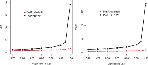
Figure 9. Graphical sketching of the results of TV and TVP provided in Table 3.

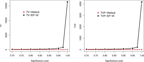
Figure 10. Graphical display of the results of VaR and TVaR provided in Table 4.

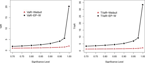
Figure 11. Graphical display of the results of TV and TVP provided in Table 4.

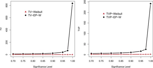
Table 2. Simulation results of the actuarial measures for the selected values of the parameters.

Dist.	Parameters	Level of significance	VaR	TVaR	TV	TVP
Weibull		0.700	1.5200	1.9853	0.1513	2.0232
		0.750	1.6255	2.0681	0.1404	2.1031
		0.800	1.7452	2.1641	0.1290	2.1964
	$\alpha =2.1$	0.850	1.8874	2.2808	0.1170	2.3101
	$\gamma =0.5$	0.900	2.0698	2.4342	0.1035	2.4601
		0.950	2.3461	2.6732	0.0867	2.6948
		0.975	2.5905	2.8898	0.0746	2.9084
		0.999	3.4924	3.7179	0.0453	3.7293
EP-W		0.700	2.3150	4.8127	78.0599	24.3277
		0.750	2.5978	5.2851	92.3318	28.3680
	$\alpha =2.1$	0.800	2.9649	5.9132	113.4390	34.2730
	$\theta =0.8$	0.850	3.4806	6.8156	147.9874	43.8125
	$\gamma =0.5$	0.900	4.3091	8.2954	215.3835	62.1413
		0.950	6.0887	11.5370	409.4976	113.9114
		0.975	8.4974	15.9801	779.0482	210.7422
		0.999	38.2903	71.5062	15,474.6648	3940.1724

Table 3. Simulation results of the actuarial measures for the selected values of the parameters.

Dist.	Parameters	Level of significance	VaR	TVaR	TV	TVP
Weibull		0.700	0.9985	1.2467	0.0410	1.2569
		0.750	1.0564	1.2906	0.0376	1.3000
		0.800	1.1214	1.3412	0.0341	1.3497
	$\alpha =2.5$	0.850	1.1977	1.4021	0.0304	1.4097
	$\gamma =1.2$	0.900	1.2942	1.4814	0.0264	1.4880
		0.950	1.4378	1.6032	0.0215	1.6085
		0.975	1.5626	1.7120	0.0181	1.7165
		0.999	2.0083	2.1163	0.0102	2.1188
EP-W		0.700	1.8512	3.3312	9.0836	5.6021
		0.750	2.0411	3.6089	10.4370	6.2182
	$\alpha =2.5$	0.800	2.2830	3.9720	12.3859	7.0685
	$\theta =1.5$	0.850	2.6155	4.4830	15.4671	8.3498
	$\gamma =1.2$	0.900	3.1343	5.2985	21.1944	10.5971
		0.950	4.2013	7.0116	36.4278	16.1186
		0.975	5.5728	9.2439	62.7387	24.9286
		0.999	19.9616	32.9239	789.0310	230.1817

Table 4. Estimated values with standard error (in parentheses) of the competing models.

Dist.	$\hat{\alpha }$	$\hat{\gamma }$	$\hat{\theta }$	$\hat{a}$	$\widehat{\text{β}}$	$\hat{c}$	$\hat{k}$
EP-W	2.353(0.0870)	0.466(0.2007)	3.488(0.7362)
Weibull	1.436(0.0458)	0.132(0.0119)
EW	0.924(0.2287)	0.721(0.0888)		4.813(1.4897)
GE		0.908(0.9936)		1.247(1.6334)
Lomax	2.548(1.1160)	3.927(1.5244)
B-XII						0.261(1.9086)	3.462(1.2383)
GOBXIII-W	2.905(1.7563)	0.975(0.8936)			1.736(2.0955)	1.084(2.1094)	3.943(1.8490)
GLM	1.487(1.6093)	0.869(0.9064)

The simulation is performed for the Weibull and EP-W for the selected values of parameters. A model with higher values of the Risk measures is said to have a heavier tail. The simulated results provided in Tables 3 and 4 show that the proposed EP-W model has higher values of the risk measures than the traditional Weibull distribution. The simulation results are graphically displayed in Figures 8–11, which show that the proposed model has heavier tail than the Weibull distribution.

8. An application to a medical care insurance data set

In this section, we use two insurance data sets to illustrate the importance and flexibility of the proposed distribution. The comparison of the proposed distribution is made with a nested model, the Weibull distribution, and with some other non-nested models such as the generalize exponential (GE), Lomax, Burr, exponentiated Weibull (EW), generalized odd Burr III-Weibull (GOBXIII-W) and generalized log-Moyal (GLM) distributions. It is important to emphasize that the EW distribution is a popular model for analysing data in the applied areas; see Mudholkar and Srivastava [29]. The GE is another non-nested model and offers the characteristics of the Weibull and gamma distributions; see Gupta and Kundu [30]. The Lomax and Burr-XII (B-XII) distributions are prominent competitors for modelling large losses and offer a wide range of applications in financial sciences. The proposed EP-W model is also compared with the GLM distribution of Bhati and Ravi [1]. We also considered the five-parameter non-nested GOBXIII-W distribution of Haq et al. [31]. The cdfs of the competing distributions are:

• The EW distribution $G\left(x;a,\alpha ,\gamma \right)={\left(1-e^{-\gamma x^{\alpha }}\right)}^a,x\ge 0,a,\alpha ,\gamma >0.$

• The GE distribution $G\left(x;a,\gamma \right)={\left(1-e^{-\gamma x}\right)}^a,x\ge 0,a,\gamma >0.$

• The Lomax distribution $G\left(x;\alpha ,\gamma \right)=1-{\left(1+\gamma x\right)}^{-\alpha },x\ge 0,\alpha ,\gamma >0.$

• The B-XII distribution $G\left(x;c,k\right)=1-{\left(1+x^c\right)}^{-k},x\ge 0,c,k>0.$

• The GOBXIII-W distribution $\begin{array}{rl}& G\left(x;\alpha ,\gamma ,\text{β},c,k\right)\\ & ={\left[1+{\left(\frac{1-{\left(1-e^{-{\left(x/\gamma \right)}^{\alpha }}\right)}^{\text{β}}}{{\left(1-e^{-{\left(x/\gamma \right)}^{\alpha }}\right)}^{\text{β}}}\right)}^c\right]}^{-k},\\ & x\ge 0,\alpha ,\gamma ,\text{β},c,k>0.\end{array}$

• The GLM distribution $G\left(x;\alpha ,\gamma \right)=erf\left(\frac{1}{\sqrt{2}}{\left(\frac{\gamma }{x}\right)}^{1/2\alpha }\right),x\ge 0,\alpha ,\gamma >0.$

Next, we consider certain analytical measures in order to verify which distribution fits better the considered data. These analytical measures include (i) discrimination measures such as Akaike information criterion (AIC), Bayesian information criterion (BIC), Hannan-Quinn information criterion (HQIC), Consistent Akaike information criterion (CAIC), and (ii) two other goodness of fit measures including Anderson–Darling (AD) test statistic and Cramer-von Mises test statistic. The discrimination measures are given by

• The AIC is $\mathrm{A}\mathrm{I}\mathrm{C}=2k-2l,$

• The BIC is $\mathrm{B}\mathrm{I}\mathrm{C}=k\log \left(n\right)-2l,$

• The HQIC $\mathrm{H}\mathrm{Q}\mathrm{I}\mathrm{C}=2k\log \left(\log \left(n\right)\right)-2l,$

• The CAIC is $\mathrm{C}\mathrm{A}\mathrm{I}\mathrm{C}=\frac{2nk}{n-k-1}-2l,$where l denotes the log-likelihood function evaluated at the MLEs, k is the number of model parameters and n is the sample size. The considered goodness of fit measures are given by

• The AD test statistic is given by $\begin{array}{rl}\mathrm{A}\mathrm{D}& =-n-\frac{1}{n}\sum _{i=1}^n\left(2i-1\right)\\ & \times \left[\log G\left(x_i\right)+\log \left\{1-G\left(x_{n-i+1}\right)\right\}\right],\end{array}$where n is the sample size and $x_i$ is the ith observation in the sample, calculated when the data is sorted in ascending order.

• The CM test statistic is given by $\mathrm{C}\mathrm{M}=\frac{1}{12n}+\sum _{i=1}^n{\left[\frac{2i-1}{2n}-G\left(x_i\right)\right]}^2.$

For the optimization and calculation of the analytical measures, we use the optim()R-function with the argument method="BFGS"; see Appendix.

8.1. Data 1: medical care insurances

Here, we illustrate the EP-W distribution by analysing a heavy-tailed data set representing medical care insurances. The data set is available at https://data.world/datasets/insurance. The maximum likelihood estimates with the standard error (in parentheses) of the fitted models for the analysed data are presented in Table 4. The analytical measures of the EP-W and other considered models are provided in Table 5. Based on the above-mentioned measures, the proposed model fits the heavy-tailed medical care insurance data set better than the other models. In support of the results provided in Table 5, the estimated pdf and cdf of the proposed distribution are plotted in Figure 12. The PP and Kaplan–Meier survival plots are sketched in Figure 13. The proposed model may be an interesting alternative to the other existing models in the literature for modelling positively skewed heavy tail data. The practical application to the medical care insurance data shows that the proposed distribution should be taken into account among other possible distributions for insurance data in which the properties of a heavy-tailed distribution are present.

Figure 12. Estimated pdf and cdf of the EP-W model corresponding to medical care insurance data.

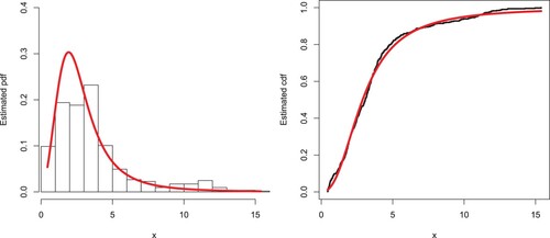
Figure 13. PP plot and Kaplan Meier survival plots of the EP-W model for the medical care insurance data.

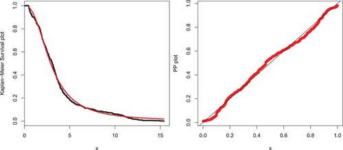
Table 5. Discrimination and goodness of fit measures of the competing models.

Dist.	AIC	BIC	CAIC	HQIC	CM	AD
EP-W	2288.154	2300.950	2288.200	2293.164	0.280	2.103
Weibull	2321.130	2329.660	2321.160	2324.477	0.943	6.249
EW	2291.085	2304.880	2292.231	2297.095	0.359	2.520
GE	2312.160	2320.956	2312.206	2315.170	0.393	2.985
Lomax	2447.169	2455.699	2447.192	2450.509	0.437	3.451
B-XII	2504.136	2512.667	2504.159	2507.477	2.744	6.786
GOBXIII-W	2302.647	2315.709	2303.634	2311.896	2.037	3.624
GLM	2298.098	2310.309	2299.091	2303.065	0.385	2.704

8.2. Data 2: vehicle insurance losses

The second data set, available at https://data.world/datasets/insurance, refers to vehicle insurance losses. The competing models are also applied to these data. The estimates with the standard error (in parentheses) of the model parameters are provided in Table 6. The analytical measures of the EP-W and other considered models are provided in Table 7. We can see that the EP-W model again outperforms all the fitted competitive models under these statistics. For the second data set, the fitted density and distribution functions of the EP-W model are plotted in Figure 14. We note that the EP-W distribution best captures the fitted pdf and cdf. The PP and Kaplan–Meier survival plots of the EP-W model are shown in Figure 15. From Figure 15, we can see that the proposed model is closely followed by the PP and Kaplan–Meier survival plots.

Figure 14. Estimated pdf and cdf plots of the EP-W distribution for the vehicle insurance loss data.

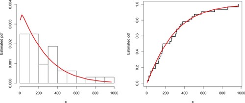
Figure 15. PP and Kaplan–Meier survival plots of the EP-W distribution for the vehicle insurance loss data.

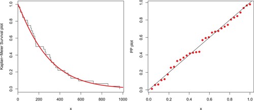
Table 6. Estimated values with standard error (in parentheses) of the competing models for data 2.

Dist.	$\hat{\alpha }$	$\hat{\gamma }$	$\hat{\theta }$	$\hat{a}$	$\widehat{\text{β}}$	$\hat{c}$	$\hat{k}$
EP-W	1.390(0.2101)	0.002(0.0008)	2.517(3.0328)
Weibull	1.019(0.9445)	0.003(1.6540)
EW	0.889(0.1315)	0.008(0.0079)		1.476(0.4897)
GE		1.234(0.2878)		0.604(0.9707)
Lomax	0.428(0.0957)	19.267(7.1664)
Burr-XII						0.056(1.1479)	3.459(7.6205)
GOBXIII-W	0.987(0.8635)	0.107(0.3848)			1.209(1.0923)	0.042(0.6323)	1.087(5.0982)
GLM	0.854(0.7498)	1.238(0.9048)

Table 7. Discrimination and goodness of fit measures of the competing models for data 2.

Dist.	AIC	BIC	CAIC	HQAIC	CM	AD
EP-W	425.490	429.887	426.347	426.947	0.044	0.115
Weibull	432.353	439.256	434.089	435.746	0.054	0.447
EW	430.226	435.623	431.083	432.683	0.049	0.183
GE	433.924	440.855	435.338	438.895	0.056	0.462
Lomax	466.167	469.099	466.581	467.139	0.204	1.215
Burr-XII	503.460	506.391	503.873	504.431	0.228	1.362
GOBXIII-W	431.220	438.618	433.897	434.678	0.054	0.359
GLM	429.908	433.097	430.654	430.324	0.051	0.259

9. Bayesian estimation

Bayesian inference procedure has been taken into consideration by many statistical researchers, especially those in the field of the survival analysis and reliability engineering. In this section, a complete sample data is analysed through Bayesian point of view. We assume that the parameters α, γ and θ of EP-W distribution have independent prior distributions as $\begin{array}{rl}\alpha & \sim \mathrm{G}\mathrm{a}\mathrm{m}\mathrm{m}\mathrm{a}(a,b),\gamma \sim \mathrm{G}\mathrm{a}\mathrm{m}\mathrm{m}\mathrm{a}(c,d),\\ \theta & \sim \mathrm{G}\mathrm{a}\mathrm{m}\mathrm{m}\mathrm{a}(e,f),\end{array}$ where a,b,c,d,e and f are positive. Hence, the joint prior density function is formulated as follow: (32) $\pi (\alpha ,\gamma ,\theta )=\frac{b^a{d}^c{f}^e}{\mathrm{\Gamma }\left(a\right)\mathrm{\Gamma }\left(c\right)\mathrm{\Gamma }\left(e\right)}{\alpha }^{a-1}{\gamma }^{c-1}{\theta }^{e-1}{e}^{-(b\alpha +d\gamma +f\theta )}.$(32) In the Bayesian estimation the actual value of the parameter, may be adversely affected by the loss when choosing an estimator. This loss can be measured by a function of the parameter and the corresponding estimator. Five well-known loss functions and associated Bayesian estimators and corresponding posterior risk are presented in Table 8.

Table 8. Bayes estimator and posterior risk under different loss functions.

Loss function	Bayes estimator	Posterior risk
$L_1=\mathrm{S}\mathrm{E}\mathrm{L}\mathrm{F}=(\theta -d{)}^2$	$E\left(\theta \right|x)$	$\mathrm{V}\mathrm{a}\mathrm{r}\left(\theta \right|x)$
$L_2=\mathrm{W}\mathrm{S}\mathrm{E}\mathrm{L}\mathrm{F}=\frac{(\theta -d{)}^2}{\theta }$	$\left(E\right({\theta }^{-1}\left|x\right){)}^{-1}$	$E\left(\theta \right|x)-(E\left({\theta }^{-1}\right|x){)}^{-1}$
$L_3=\mathrm{M}\mathrm{S}\mathrm{E}\mathrm{L}\mathrm{F}={\left(1-\frac{d}{\theta }\right)}^2$	$\frac{E\left({\theta }^{-1}\right|x)}{E\left({\theta }^{-2}\right|x)}$	$1-\frac{E\left({\theta }^{-1}\right|x{)}^2}{E\left({\theta }^{-2}\right|x)}$
$L_4=\mathrm{P}\mathrm{L}\mathrm{F}=\frac{(\theta -d{)}^2}{d}$	$\sqrt{E\left({\theta }^2\right|x)}$	$2\left(\sqrt{E\left({\theta }^2\right|x)}-E\left(\theta \right|x)\right)$
$L_5=\mathrm{K}\mathrm{L}\mathrm{F}=\left(\sqrt{\frac{d}{\theta }-\sqrt{\frac{\theta }{d}}}\right)$	$\sqrt{\frac{E\left(\theta \right|x)}{E\left({\theta }^{-1}\right|x)}}$	$2\left(\sqrt{E\left(\theta \right|x\left)E\right({\theta }^{-1}\left|x\right)}-1\right)$

For more details see Calabria and Pulcini [32]. Next, we provide the posterior probability distribution for a complete data set. We define the function ϕ as $\begin{array}{rl}\varphi (\alpha ,\gamma ,\theta )& ={\alpha }^{a-1}{\gamma }^{c-1}{\theta }^{e-1}{e}^{-(b\alpha +d\gamma +f\theta )},\\ & \alpha >0,\gamma >0,\theta >0.\end{array}$ The joint posterior distribution in terms of a given likelihood function $L\left(\mathrm{d}\mathrm{a}\mathrm{t}\mathrm{a}\right)$ and joint prior distribution $\pi (\alpha ,\gamma ,\theta )$ is defined as (33) ${\pi }^{\ast }(\alpha ,\gamma ,\theta |\mathrm{d}\mathrm{a}\mathrm{t}\mathrm{a})\propto \pi (\alpha ,\gamma ,\theta )L\left(\mathrm{d}\mathrm{a}\mathrm{t}\mathrm{a}\right).$(33) Hence, we obtain the joint posterior density of the parameters α, γ and θ for the complete sample data by combining the likelihood function and the joint prior density (33(33) ${\pi }^{\ast }(\alpha ,\gamma ,\theta |\mathrm{d}\mathrm{a}\mathrm{t}\mathrm{a})\propto \pi (\alpha ,\gamma ,\theta )L\left(\mathrm{d}\mathrm{a}\mathrm{t}\mathrm{a}\right).$(33) ). Therefore, the joint posterior density function is given by (34) ${\pi }^{\ast }(\alpha ,\gamma ,\theta |\underset{\_}{x})=K\varphi (\alpha ,\gamma ,\theta )\prod _{i=1}^n\frac{\alpha \theta \gamma x_i^{\alpha -1}\exp \left(\frac{\gamma x_i^{\alpha }}{\theta +\gamma x_i^{\alpha }}\right)}{(\theta +\gamma x_i^{\alpha }{)}^2},$(34) where K is given by $\begin{array}{rl}{K}^{-1}& ={\int }_0^{\mathrm{\infty }}{\int }_0^{\mathrm{\infty }}{\int }_0^{\mathrm{\infty }}\varphi (\alpha ,\gamma ,\eta )\\ & \times \prod _{i=1}^n\frac{\alpha \theta \gamma x_i^{\alpha -1}\exp \left(\frac{\gamma x_i^{\alpha }}{\theta +\gamma x_i^{\alpha }}\right)}{(\theta +\gamma x_i^{\alpha }{)}^2}\mathrm{d}\alpha \mathrm{d}\gamma \mathrm{d}\theta .\end{array}$ It is clear from Equation (34) that there is no closed form for the Bayesian estimators under the Five loss functions described in Table 8(8) $G\left(x\right)=\frac{\cos \left[\frac{\pi }{2}\left\{1-F{\left(x;\xi \right)}^a\right\}\right]}{1-\log \left[1-F{\left(x;\xi \right)}^a\right]},a>0,x\in \mathbb{R}.$(8) , so we suggest using a MCMC procedure based on 10,000 replicates to compute Bayesian estimators. The corresponding Bayesian estimates and posterior risk are provided in Table 9. Table 10 provides $95\mathrm{\%}$ credible and HPD intervals for each parameter of the EP-W distribution. The posterior samples extracted by using Gibbs sampling technique. Moreover, we provide the posterior summary plots in Figures 16–18. These plots confirm that the sampling process is of the prime quality and the convergence does occur.

Figure 16. Plots of Bayesian analysis and performance of Gibbs sampling for Insurance data set. Trace plots of each parameter of EP-W distribution.

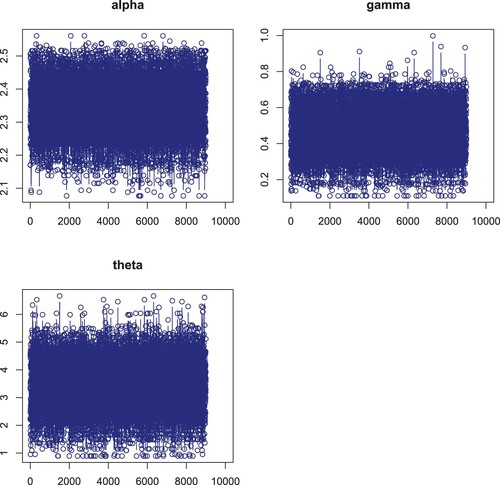
Figure 17. Plots of Bayesian analysis and performance of Gibbs sampling for Insurance data set. Autocorrelation plots of each parameter of EP-W distribution.

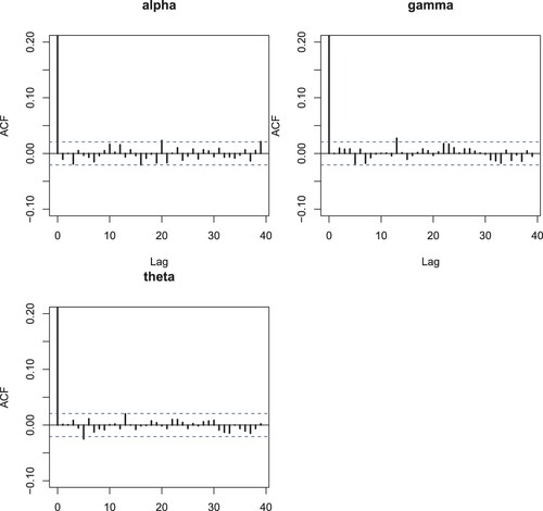
Figure 18. Plots of Bayesian analysis and performance of Gibbs sampling for Insurance data set. Histogram plots of each parameter of EP-W distribution.

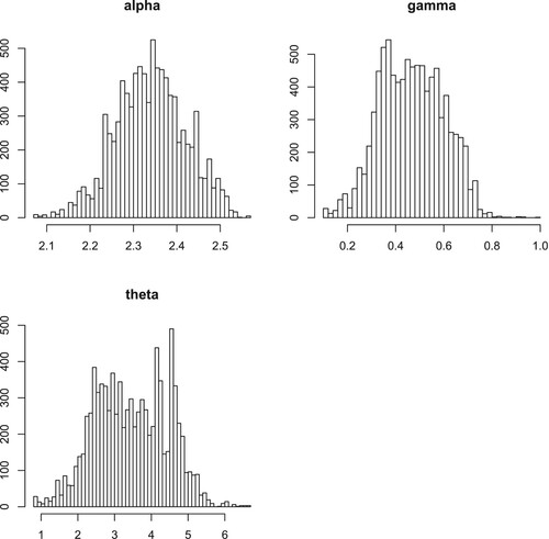
Table 9. Bayesian estimates and their posterior risks of the parameters under different loss functions based on the medical care insurance data.

	$\hat{\alpha }$		$\hat{\gamma }$		$\hat{\theta }$
Bayes loss functions	Estimate	Risk	Estimate	Risk	Estimate	Risk
SELF	2.3404	0.0065	0.4666	0.0174	3.4543	0.9733
WSELF	2.3376	0.0028	0.4226	0.0440	3.1250	0.3293
MSELF	2.3348	0.0012	0.3695	0.1257	2.7428	0.1223
PLF	2.3418	0.0028	0.4849	0.0366	3.5924	0.2762
KLF	2.3390	0.0012	0.4440	0.1015	3.2855	0.1028

Table 10. Credible and HPD intervals of the parameters α, γ and θ for the medical care insurance data.

Parameters	Credible interval	HPD interval
α	(2.284, 2.395)	(2.201, 2.516)
γ	(0.364, 0.566)	(0.2507,0.7267)
θ	(2.681, 4.222)	(1.649, 5.197)

For the vehicle insurance losses, the Bayesian estimates along with corresponding the posterior risk are provided in Table 11. Table 12 provides $95\mathrm{\%}$ credible and HPD intervals for each parameter of the EP-W distribution. The posterior samples extracted by using Gibbs sampling technique. Corresponding to the vehicle insurance data set, the posterior summary plots are provided in Figures 19–21. These plots confirm that the sampling process is of the prime quality and the convergence does occur.

Figure 19. Plots of Bayesian analysis and performance of Gibbs sampling for Insurance data set. Trace plots of each parameter of EP-W distribution for the vehicle insurance losses data.

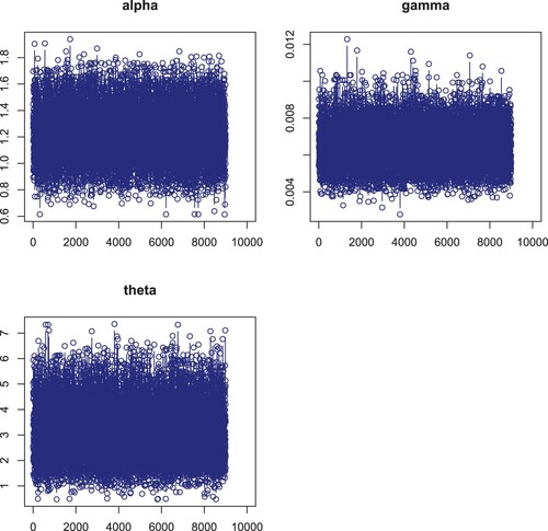
Figure 20. Plots of Bayesian analysis and performance of Gibbs sampling for Insurance data set. Autocorrelation plots of each parameter of EP-W distribution.

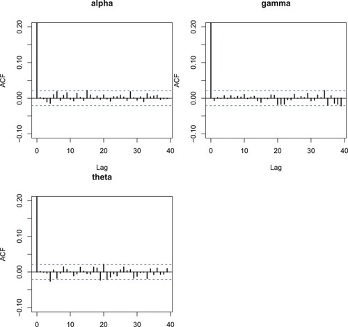
Figure 21. Plots of Bayesian analysis and performance of Gibbs sampling for Insurance data set. Histogram plots of each parameter of EP-W distribution.

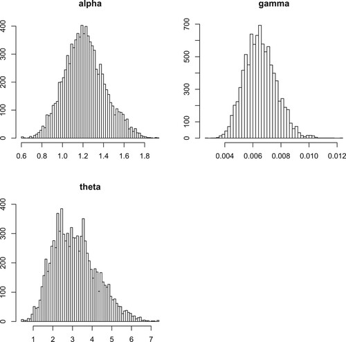
Table 11. Bayesian estimates and their posterior risks of the parameters under different loss functions based on the vehicle insurance losses data.

	$\hat{\alpha }$		$\hat{\gamma }$		$\hat{\theta }$
Bayes Loss functions	Estimate	Risk	Estimate	Risk	Estimate	Risk
SELF	1.3047	0.0307	0.0080	0.4389	3.2091	1.5498
WSELF	1.2826	0.0220	0.0026	0.0054	2.7037	0.5055
MSELF	1.2618	0.0162	0.0020	0.9001	2.2058	0.1841
PLF	1.3164	0.0235	0.0104	0.0048	3.4422	0.4660
KLF	1.2936	0.0171	0.0045	0.5253	2.9456	0.1789

Table 12. Credible and HPD intervals of the parameters α, γ and θ for the vehicle insurance losses data.

Parameters	Credible interval	HPD interval
α	(1.190, 1.392)	(0.971, 1.669)
γ	(0.003, 0.011)	(0.007, 0.021)
θ	(2.264, 3.978)	(0.958, 5.579)

10. Concluding remarks

To cater data in financial and actuarial sciences, a number of methods to define heavy-tailed distributions have been proposed. In this regard, we further carried this branch of distribution theory and proposed nine new families of distributions. A three-parameter special model, called EP-W distribution, is studied in detail. Some mathematical properties along with certain characterizations are derived. Actuarial measures of the proposed model are also calculated and a simulation study has been conducted to show the usefulness of the proposed method in actuarial sciences. To prove the potential of the EP-W distribution, we considered two insurance data sets and compared its goodness of fit with other well-known distributions. The proposed distribution outclassed the competitive models by considering certain analytical measures. We hope that the new development will attract wider applications in the financial and insurance sciences and would be quite helpful for the new comers in the field of distribution theory.

Acknowledgments

The authors are grateful to the Editor-in-Chief, the Associate Editor and the anonymous referees for many of their valuable comments and suggestions which lead to this improved version of the paper. The first two authors also acknowledge the support of the Yazd University, Iran.

Disclosure statement

This article is drafted from the Ph.D work of Mr. Zubair Ahmad.

Data availability statement

This work is mainly a methodological development and has been applied on secondary data related to financial and insurance sciences, but if required, data will be provided.

Appendix

Theorem A.1

Let $(\mathrm{\Omega },\mathcal{F},\mathbf{P})$ be a given probability space and let $H=[d,e]$ be an interval for some d<e ($d=-\mathrm{\infty },e=\mathrm{\infty }$ might as well be allowed). Let $X:\mathrm{\Omega }\to H$ be a continuous random variable with the distribution function F and let $q_1$ and $q_2$ be two real functions defined on H such that $\mathbf{E}\left[q_2\left(X\right)|X\ge x\right]=\mathbf{E}\left[q_1\left(X\right)|X\ge x\right]\eta \left(x\right),x\in H,$ is defined with some real function η. Assume that $q_1,q_2\in C^1\left(H\right),$ $\eta \in C^2\left(H\right)$ and F is twice continuously differentiable and strictly monotone function on the set H. Finally, assume that the equation $\eta q_1=q_2$ has no real solution in the interior of H. Then F is uniquely determined by the functions $q_1,q_2$ and η, particularly $F\left(x\right)={\int }_a^{x}C\left|\frac{{\eta }^{\mathrm{\prime }}\left(u\right)}{\eta \left(u\right)q_1\left(u\right)-q_2\left(u\right)}\right|\exp \left(-s\left(u\right)\right)\mathrm{d}u,$ where the function s is a solution of the differential equation $s^{\mathrm{\prime }}={\eta }^{\mathrm{\prime }}{q}_1/\eta q_1-q_2$ and C is the normalization constant, such that ${\int }_H\mathrm{d}F=1$.

We like to mention that this kind of characterization based on the ratio of truncated moments is stable in the sense of weak convergence (see, Glänzel [27]), in particular, let us assume that there is a sequence $\left\{X_n\right\}$ of random variables with distribution functions $\left\{F_n\right\}$ such that the functions $q_{1n}$, $q_{2n}$ and ${\eta }_n(n\in \mathbb{N})$ satisfy the conditions of Theorem A.1 and let $q_{1n}\to q_1$, $q_{2n}\to q_2$ for some continuously differentiable real functions $q_1$ and $q_2$. Let, finally, X be a random variable with distribution F. Under the condition that $q_{1n}\left(X\right)$ and $q_{2n}\left(X\right)$ are uniformly integrable and the family $\left\{F_n\right\}$ is relatively compact, the sequence $X_n$ converges to X in distribution if and only if ${\eta }_n$ converges to η, where $\eta \left(x\right)=\frac{E\left[q_2\left(X\right)|X\ge x\right]}{E\left[q_1\left(X\right)|X\ge x\right]}.$ This stability theorem makes sure that the convergence of distribution functions is reflected by corresponding convergence of the functions $q_1,q_2$ and η, respectively. It guarantees, for instance, the “convergence” of characterization of the Wald distribution to that of the Lévy–Smirnov distribution if $\alpha \to \mathrm{\infty }$. A further consequence of the stability property of Theorem A.1 is the application of this theorem to special tasks in statistical practice such as the estimation of the parameters of discrete distributions. For such purpose, the functions $q_1,q_2$ and, specially, η should be as simple as possible. Since the function triplet is not uniquely determined it is often possible to choose η as a linear function. Therefore, it is worth analysing some special cases which helps to find new characterizations reflecting the relationship between individual continuous univariate distributions and appropriate in other areas of statistics. In some cases, one can take $q_1\left(x\right)\equiv 1,$ which reduces the condition of Theorem A.1 to $\mathbf{E}\left[q_2\right(X)|X\ge x]=\eta \left(x\right),x\in H$. We, however, believe that employing three functions $q_1,q_2$ and η will enhance the domain of applicability of Theorem A.1.

R Code for analysis

Note: In the following R-code, a is used for α, t is used for θ, g is used for γ and pm is used for proposed model.

References

- Bhati D, Ravi S. On generalized log-Moyal distribution: a new heavy tailed size distribution. Insur Math Econ. 2018;79:247–259. doi: 10.1016/j.insmatheco.2018.02.002
- Beirlant J, Matthys G, Dierckx G. Heavy-tailed distributions and rating. ASTIN Bull. 2001;31(1):37–58. doi: 10.2143/AST.31.1.993
- McNeil AJ. Estimating the tails of loss severity distributions using extreme value theory. ASTIN Bull. 1997;27(1):117–137. doi: 10.2143/AST.27.1.563210
- Resnick SI. Discussion of the Danish data on large fire insurance losses. ASTIN Bull. 1997;27(1):139–151. doi: 10.2143/AST.27.1.563211
- Eling M. Fitting insurance claims to skewed distributions: are the skew-normal and skew-student good models. Insur Math Econ. 2012;51(2):239–248. doi: 10.1016/j.insmatheco.2012.04.001
- Adcock C, Eling M, Loperfido N. Skewed distributions in finance and actuarial science: a review. Eur J Financ. 2015;21(13-14):1253–1281. doi: 10.1080/1351847X.2012.720269
- Shushi T. Skew-elliptical distributions with applications in risk theory. Eur Actuar J. 2017;7:277–296. doi: 10.1007/s13385-016-0144-9
- Punzo A. A new look at the inverse Gaussian distribution with applications to insurance and economic data. J Appl Stat. 2019;46(7):1260–1287. doi: 10.1080/02664763.2018.1542668
- Azzalini A, Del Cappello T, Kotz S. Log-skew-normal and log-skew-t distributions as models for family income data. J Inco Dist. 2002;11:12–20.
- Bagnato L, Punzo A. Finite mixtures of unimodal beta and gamma densities and the k-bumps algorithm. Comput Stat. 2013;28(4):1571–1597. doi: 10.1007/s00180-012-0367-4
- Paula GA, Leiva V, Barros M, et al. Robust statistical modeling using the Birnbaum Saunders t distribution applied to insurance. Appl Stoch Models Bus Ind. 2012;28(1):16–34. doi: 10.1002/asmb.887
- Klugman SA, Panjer HH, Willmot GE. Loss models: from data to decisions. 4th ed. John Wiley and Sons, Inc; 2012. (Wiley series in probability and statistics).
- Nadarajah S, Abu Bakar SA. New composite models for the Danish fire insurance data. Scand Actuar J. 2014;2014(2):180–187. doi: 10.1080/03461238.2012.695748
- Bakar SA, Hamzah N, Maghsoudi M, et al. Modeling loss data using composite models. Insur Math Econ. 2015;61:146–154. doi: 10.1016/j.insmatheco.2014.08.008
- Punzo A, Bagnato L, Maruotti A. Compound unimodal distributions for insurance losses. Insur Math Econ. 2018;81:95–107. doi: 10.1016/j.insmatheco.2017.10.007
- Mazza A, Punzo A. Modeling household income with contaminated unimodal distributions. In: Petrucci A, Racioppi F, Verde R, editors. New statistical developments in data science; 2019. p. 373–391. (Springer proceedings in mathematics & statistics; vol. 288).
- Tahir MH, Cordeiro GM. Compounding of distributions: a survey and new generalized classes. J Stat Distrib Appl. 2016;3(1):1–35. doi: 10.1186/s40488-016-0052-1
- Bernardi M, Maruotti A, Petrella L. Skew mixture models for loss distributions: a Bayesian approach. Insur Math Econ. 2012;51(3):617–623. doi: 10.1016/j.insmatheco.2012.08.002
- Miljkovic T, Grr̈n B. Modeling loss data using mixtures of distributions. Insur Math Econ. 2016;70:387–396. doi: 10.1016/j.insmatheco.2016.06.019
- Punzo A, Mazza A, Maruotti A. Fitting insurance and economic data with outliers: a flexible approach based on finite mixtures of contaminated gamma distributions. J Appl Stat. 2018;45(14):2563–2584. doi: 10.1080/02664763.2018.1428288
- Dutta K, Perry J. A tale of tails: an empirical analysis of loss distribution models for estimating operational risk capital. New Engl Econ Rev. 2006;6(13):1–85.
- Alzaatreh A, Lee C, Famoye F. A new method for generating families of continuous distributions. Metron. 2013;71(1):63–79. doi: 10.1007/s40300-013-0007-y
- Ahmad Z, Hamedani GG, Butt NS. Recent developments in distribution theory: a brief survey and some new generalized classes of distributions. Pak J Stat Oper Res. 2019;15(1):87–110. doi: 10.18187/pjsor.v15i1.2803
- Jamal F, Nasir M. Some new members of the T-X family of distributions. Proceedings of the 17th International Conference on Statistical Sciences; 2019 Jan; Lahore, Pakistan. <hal-01965176v2>.
- Mahdavi A, Kundu D. A new method for generating distributions with an application to exponential distribution. Commun Stat-Theory M. 2017;46(13):6543–6557. doi: 10.1080/03610926.2015.1130839
- Glänzel W. A characterization theorem based on truncated moments and its application to some distribution families. Mathematical Statistics and Probability Theory. Dordrecht: Springer; 1987. p. 75-84.
- Glänzel W. Some consequences of a characterization theorem based on truncated moments. Statistics. 1990;21(4):613–618. doi: 10.1080/02331889008802273
- Artzner P. Application of coherent risk measures to capital requirements in insurance. N Am Actuar J. 1999;3(2):11–25. doi: 10.1080/10920277.1999.10595795
- Mudholkar GS, Srivastava DK. Exponentiated Weibull family for analyzing bathtub failure-rate data. IEEE Trans Reliab. 1993;42(2):299–302. doi: 10.1109/24.229504
- Gupta RD, Kundu D. Exponentiated exponential family: an alternative to gamma and Weibull distributions. Biom J. 2001;43(1):117–130. doi: 10.1002/1521-4036(200102)43:1<117::AID-BIMJ117>3.0.CO;2-R
- Haq MAU, Elgarhy M, Hashmi S. The generalized odd Burr III family of distributions: properties, applications and characterizations. J Taibah Univ Sci. 2019;13(1):961–971. doi: 10.1080/16583655.2019.1666785
- Calabria R, Pulcini G. Point estimation under asymmetric loss functions for left-truncated exponential samples. Comm Statist Theory Methods. 1996;25(3):585–600. doi: 10.1080/03610929608831715
Appendix
Theorem A.1
Let be a given probability space and let
be an interval for some d<e (
might as well be allowed). Let
be a continuous random variable with the distribution function F and let
and
be two real functions defined on H such that
is defined with some real function η. Assume that
and F is twice continuously differentiable and strictly monotone function on the set H. Finally, assume that the equation
has no real solution in the interior of H. Then F is uniquely determined by the functions
and η, particularly
where the function s is a solution of the differential equation
and C is the normalization constant, such that