Analytic approximate solutions for some nonlinear Parabolic dynamical wave equations

Abstract

In this paper, modified variational iteration algorithm-II is investigated for finding approximate solutions of nonlinear Parabolic equations. Comparisons of the MVIA-II with trigonometric B-spline collocation method, variational iteration method, homotopy perturbation transform method, Adomian decomposition method, and modified variational iteration method are carried out, which show that the proposed algorithm (MVIA-II) is robust one. Some nonlinear Parabolic equations are given to demonstrate the implementation and accuracy of the MVIA-II.

KEYWORDS:

• Modified variational iteration algorithm-II
• Newell–Whitehead equation
• Fisher equations
• Allen-Cahn equation
• MVIA-I

1. Introduction

The exceptional advancement of nonlinear sciences and engineering during the most recent two decades, several analytical and numerical methods [1,2] including the sine-Gordon expansion, Adomian's decomposition [1], Finite difference [2], Variational iteration algorithm-I [5], Backlund transformation, Homotopy Pade [3], Variational principle [4], Jacobi elliptic function expansion [5], implicit-explicit [6], tanh-coth [7], Homotopy Analysis [8], Fourier pseudo-spectral [9], Hirota's bilinear [10], Homotopy Perturbation [11], Finite volume [12], lattice Boltzmann [13], generalized $\left(G^{\mathrm{\prime }}/G\right)-$ expansion method [14,15] are presented to solve different type differential equations. Most of these approaches have their inbuilt insufficiencies including divergent results, calculation of Adomian's polynomials, un-realistic assumptions, limited convergence, very lengthy calculations and non-compatibility with the nonlinearity of physical problem [16]. Encouraged and inspired by the continuous study in this area, we employ a moderately new strategy which is called modified variational iteration algorithm-II to find the mathematical solution of the general nonlinear parabolic equation [17] arises in quantum mechanics, plasma physics and mathematical biology of the form (1) $\frac{\mathrm{\partial }v}{\mathrm{\partial }t}=\frac{{\mathrm{\partial }}^{2}v}{\mathrm{\partial }{x}^2}+\alpha v+\text{β}{v}^n,$(1) where $\alpha \text{and}\text{β}$ are non zero real constants. Equation (1) gives rise to three widely known models. It becomes Allen-Cahn equation when $n=3,\alpha =1\text{and}\text{β}=-1$, which has various applications in quantum mechanics, biology and plasma physics [18]. If for $\text{β}=-\text{β}\text{and}n=3$, then Equation (1) turn out to be Newell–Whitehead (NW) equation, which appears in various study for describing the Rayleigh -Benard convection of binary fluid mixtures. While for $n=2\text{and}\text{β}=-\alpha$ this equation reduced to Fishers equation.

The AC equation is the indispensable model for numerous physical phenomena and helps as a model for the study of separation of phase in binary, isotropic and isothermal mixtures. It is well notorious that wave phenomena of fluid dynamics are demonstrated by bell-shaped $\text{sec}h$ or $\text{tan}h$ solutions and kink shaped solutions. To find analytical as well as numerical solutions of this model, numerous approaches can be found in the literature like the finite difference method has been applied by Yokuş and Bulut [19] for the mathematical computation of Ac equation and has been shown that the proposed technique is more stable than the Fourier-Von Neumann technique for solving these type equations. Hariharan and Kannan [17] developed Haar wavelet or transform technique for this type equations, Bulut et al. [20] used Bernoulli sub-equation function technique to gain exponential prototype structures to the AC model. Yang et al. [6] studied the stability of the Implicit-Explicit approaches for AC equation [37], Gui and Zhao [21] studied the qualitative properties of travelling wave solution of the AC equation. Jeong and Kim [22] proposed an explicit hybrid numerical method based on splitting technique and obtained analytical solution of Allen-Cahn equation, while the combination of Quasi-Newton, reproducing kernel and finite difference methods are utilized by Niu et al. [23]. Hou and Leng [23] considered a finite difference technique for the approximations of one-dimensional AC equation. Recently, Chen et al. [24] derived a posteriori error approximation based on the elliptic reconstruction method for AC equation by applying Crank–Nicolson finite element technique.

The Newell-Whitehead equation which is also known as Newell–Whitehead–Segel equation explains the dynamical behaviour near the bifurcation point for the Rayleigh-Benard convection of binary fluid mixtures [7]. In recent years, many authors have studied this equation and for the numerical solution of this type equation, different approaches have been employed like Ezzati and Shakibi [25] applied multiquadric quasi-interpolation and Adomian's decomposition methods for the numerical treatment of NW equation. Homotopy Pade and Homotopy analysis methods have been employed by Kheiri et al. [3], Sakaguchi [26] studied Zigzag instability of the NW equation numerically, while, Antoniou [27] obtained analytic solution of the NW equation by using Riccati equation method.

The well-known Fisher's equation combines logistic nonlinearity with diffusion. It was Fisher [28] who presented for the first time, the renowned equation is known as Fisher equation, to define the propagation of a mutant gene, which has many applications and encountered in population dynamics, chemical kinetics, flame propagation, neurophysiology and autocatalytic chemical reactions [29–31]. Many researchers have explained this model by different methods like Harihar an et al. [32] have presented Haar wavelet technique for the mathematical treatment of Fisher's equation. Homotopy analysis technique has been employed for the analytical solution of Fisher equation by Babolian and Saeidian [8]. Ismail et al. [1] have employed Adomian decomposition technique for the approximate solution, Zhang et al. [33] employed discontinuous Galerkin technique for numerical solution, Moghimi and Hejazi [34] have used Variational iteration method and by Modified pseudospectral method is investigated by Javidi [35]. Triki and Wazwaz [36] proposed a trial equation method for exact soliton solutions have been obtained for the first time of the Fisher equation. It is worth referencing that Wazwaz made a nitty-gritty investigation for solitons and kink solutions of Newell–Whitehead, Allen-Cahn and Fisher equations using tanh–coth approach [7] and analytical solutions of these equations are attained by Adomian decomposition method [37].

In the last two decades, the variational iteration method has been broadly employed for the analytic approximate solutions of different types of PDEs [38–43]. The originator himself advanced this method and now variational iteration algorithms have attracted more researchers. These algorithms are employed as an alternative to obtain a precise and a reliable solution of the nonlinear PDEs models which reduce complexities counter in the process conventional methods like finite element procedures, finite difference and, Adomian decomposition method etc. [44–53].

The main endeavour of this article is to introduce a numerical algorithm to approximate the Newell–Whitehead (NW), Allen–Cahn (AC) and Fisher's equations. It is to be worth mentioning that such model equations arise commonly in various branches of science, engineering and physics, the proposed algorithm is completely well-suited with the complications of such problems as well as easy to implement and use. Numerical results are very accurate and encouraging.

This article is composed as follows; in Section [2], modified variational iteration algorithm-II is depicted. In Section [3], To check the dependability of new presented technique, some problems are incorporated and results are shown in the form of absolute error for various values of parameters used in the models, and in the last segment [4], a nitty gritty conclusion is discussed.

2. Description of the method

In order to convey the elementary idea of MVIA-II, we consider. (2) $L\left(v\right)+N\left(v\right)=g,$(2) where $L\left(v\right)$ is a linear, $N\left(v\right)$ is a nonlinear operator and $g$ is the source term. For any nonzero scalar $\lambda$, we have (3) $\lambda \left[L\left(v\right)+N\left(v\right)-g\right]=0,$(3) By taking the integral from 0 to $\varsigma$, we get, (4) ${\int }_0^{\varsigma }\lambda \left[L\left(v\right)+N\left(v\right)-g\right]ds,$(4) The above relation can be rewritten as: (5) $v_n\left(\varsigma \right)=v_n\left(\varsigma \right)+{\int }_0^{\varsigma }\lambda \left[L\left(v\right)+N\left(v\right)-g\right]ds,$(5) From Equation (5), one can find The relation of recurrence of VIM given below, (6) $v_{n+1}\left(\varsigma \right)=v_n\left(\varsigma \right)+{\int }_0^{\varsigma }\left[L\left\{v_n\left(s\right)\right\}+N\left\{v_n\left(s\right)\right\}-g\right]ds,$(6)

For a given $v_0\left(\varsigma \right)$, approximate solution $v_{n+1}\left(\varsigma \right)$ of equation (5) can be obtained, and the Equation (6) is known as variational iteration method, where the unknown scalar $\lambda$ is known as the Lagrange multiplier [54], its values can be obtained by using the optimality conditions. (7) $v_{n+1}\left(\varsigma \right)=v_n\left(\varsigma \right)+{\int }_0^{\varsigma }\lambda \left[L\left\{v_n\left(s\right)\right\}+\widetilde{N\left\{v_n\left(s\right)\right\}}-g\right]ds,$(7) In the above recurrence relation $\widetilde{v_n\left(s\right)}$ is considered as a restricted variation. which in turn gives $\delta \widetilde{v_n\left(s\right)}=0$.

According to He et al. [55,56], a more summarizing iteration formula can be made, known as variational iteration algorithm-II (VIA-II), (8) $v_{n+1}\left(\varsigma \right)=v_0\left(\varsigma \right)+{\int }_0^{\varsigma }\lambda \left[N\left\{v_n\left(s\right)\right\}-g\right]ds,$(8) The sequence of approximants obtained gives us the exact solution $v\left(\varsigma \right)$, where (9) $v\left(\varsigma \right)={\text{Lim}}_{n\to \mathrm{\infty }}{v}_n\left(\varsigma \right).$(9) An auxiliary parameter $h$ can be presented into the iterative algorithm: VIA-II, which is employed to improve the accurateness and ability of the procedure. By introducing $h$, in MVIA-II and summarizing the procedure; (10) $\left\{\begin{array}{l}{v}_0\left(\varsigma \right)\text{is}\text{a}\text{proper}\text{initial}\text{approximation},\\ v_1\left(\varsigma ,h\right)=v_0\left(\varsigma \right)+h{\int }_0^{\varsigma }\lambda \left(s\right)\left[L\right\{v_0\left(s\right)\}\\ +N\left\{v_0\left(s\right)\right\}-g\left(s\right)]ds,\\ v_{n+1}\left(\varsigma ,h\right)=v_0\left(\varsigma ,h\right)+h{\int }_0^{\varsigma }\lambda \left(s\right)\\ \left[N\left\{v_n\left(s,h\right)\right\}-g\left(s,h\right)\right]ds,\\ n=1,2,3,\dots \end{array}\right.$(10) This algorithm is named as MVIA-II and utilized here to investigate some nonlinear Parabolic equations numerically.

3. Numerical applications

In order to demonstrate the implementation, precision and effectiveness of the planned algorithm, five different types of nonlinear Parabolic equations have been solved in this section. Two test problems are for Allen–Cahn equation, two for Newell–Whitehead equation and the other one test problem is for the Fisher equation. We compute the absolute error described by the below relation $E_j=|v_j^{\text{exact}}-V_j^{\text{approximate}}|.$Also, all the numerical computation work has been made by using Mapple and Matlab R2015a.

3.1. Test Problem 1 (Allen–Cahn equation)

First, consider the Equation (1) with the values of constants as $n=3,\alpha =1\text{and}\text{β}=-1$, which gives the AC equation of the following form [57], (11) $\frac{\mathrm{\partial }v}{\mathrm{\partial }t}=\frac{{\mathrm{\partial }}^{2}v}{\mathrm{\partial }{x}^2}+v-v^3,$(11)

With initial-boundary conditions: $\begin{array}{rl}v\left(x,0\right)& =-0.5+0.5\tan h\left(0.3536x\right),\\ v\left(0,t\right)& =-0.5+0.5\tan h\left(0.75t\right).\end{array}$ $v\left(1,t\right)=-0.5+0.5\tan h\left(0.3536-0.75t\right),$The exact solution of the above system as follows from [57]: (12) $v\left(x,t\right)=-0.5+0.5\text{tan}h\left(0.3536x-0.75t\right).$(12)

The relation of recurrence of VIM for Equation (11) is given by, (13) $\begin{array}{rl}{v}_{n+1}\left(x,t,h\right)& =v_n\left(x,t,h\right)+h{\int }_0^t\lambda \left(\varsigma \right)\\ & \times \left\{\frac{\mathrm{\partial }{v}_n\left(x,\varsigma ,h\right)}{\mathrm{\partial }\varsigma }-\stackrel{~}{\frac{{\mathrm{\partial }}^2{v}_n\left(x,\varsigma ,h\right)}{\mathrm{\partial }{x}^2}}\right.\\ & \left.-\widetilde{v_n\left(x,\varsigma ,h\right)+}\widetilde{v_n{\left(x,\varsigma ,h\right)}^3}\phantom{\frac{\mathrm{\partial }{v}_n\left(x,\varsigma ,h\right)}{\mathrm{\partial }\varsigma }}\right\}d\varsigma ,\end{array}$(13) The value of $\lambda \left(\varsigma \right)$ can be obtained by the variational principle [58–60] or using the optimality condition, $\frac{\mathrm{\partial }{v}_{n+1}\left(x,t,h\right)}{\mathrm{\partial }{v}_n\left(x,t,h\right)}=0$We obtained the value of $\lambda \left(\varsigma \right)$, which is $\lambda \left(\varsigma \right)=-1$. By putting the value of $\lambda \left(\varsigma \right)$ in equation (13) gives (14) $\begin{array}{rl}{v}_{n+1}\left(x,t,h\right)& =v_n\left(x,t,h\right)+h{\int }_0^t\lambda \left(\varsigma \right)\left\{\frac{\mathrm{\partial }{v}_n\left(x,\varsigma ,h\right)}{\mathrm{\partial }\varsigma }\right.\\ & -\frac{{\mathrm{\partial }}^2{v}_n(x,\varsigma ,h)}{\mathrm{\partial }{x}^2}-v_n(x,\varsigma ,h)\\ & +\left.v_n\left(x,\varsigma ,h{)}^3\right)\phantom{\frac{{\mathrm{\partial }}^2{v}_n(x,\varsigma ,h)}{\mathrm{\partial }{x}^2}}\right\}d\varsigma ,\end{array}$(14)

According to our proposed scheme (10), the following iterative formula is obtained (15) $\begin{array}{rl}{v}_{n+1}\left(x,t,h\right)& =v_0\left(x,t,h\right)+h{\int }_0^t\lambda \left(\varsigma \right)\left\{-\frac{{\mathrm{\partial }}^2{v}_n\left(x,\varsigma ,h\right)}{\mathrm{\partial }{x}^2}\right.\\ & \left.-v_n\left(x,\varsigma ,h\right)+v_n{\left(x,\varsigma ,h\right)}^3)\phantom{\frac{{\mathrm{\partial }}^2{v}_n\left(x,\varsigma ,h\right)}{\mathrm{\partial }{x}^2}}\right\}d\varsigma ,\end{array}$(15) We consider the initial approximation $v_0\left(x,t\right)$ as, $v_0\left(x,t\right)=-0.5+0.5\tan h\left(0.3536x\right).$Then from The relation of recurrence of VIM (14), we get the following other iterations, $\begin{array}{rl}{v}_1(x,t,h)& =\text{tan}h\left(\right(221\ast x\left)/625\right)/2\\ & -(h\ast t\ast \text{exp}((442\ast x)/625)\\ & \ast (585989\ast \text{exp}(442\ast x\left)/625\right)\\ & +585886\left)\right)/(390625\ast \text{exp}((442\ast x)/625)\\ & +1{)}^{\wedge }3-1/2,\end{array}$ $⋮$ $⋮$

For obtained approximate solution, the following residual function can be used to find a valid value of h, (16) $\begin{array}{rl}{r}_3\left(x,t,h\right)& =\frac{\mathrm{\partial }{v}_3\left(x,t,h\right)}{\mathrm{\partial }t}-\frac{{\mathrm{\partial }}^2{v}_3\left(x,t,h\right)}{\mathrm{\partial }{x}^2}\\ & -v_3\left(x,t,h\right)+v_3(x,t,h{)}^3.\end{array}$(16)

The norm 2 of residual function (16) for 3rd-order approximate solution for $\left(x,t\right)ϵ\left[0,1\right]\times \left[0,1\right]$ is (17) $e_3\left(h\right)={\left[\frac{1}{{\left(11\right)}^2}\sum _{i=0}^{10}\sum _{j=0}^{10}{\left\{r_3\left(\frac{i}{10},\frac{j}{10},h\right)\right\}}^2\right]}^{\frac{1}{2}}$(17)

The residual function (17) can be utilized for the approximation of $e_3\left(h\right)$ and an appropriate value of the $h$ can be found out by making the $e_3\left(h\right)$ minimum. The value of the auxiliary parameter is determined to be 0.956746100718808 when the minimum value of $e_3\left(h\right)$ is obtained which is 0.768386328622880561E-3. More precise and accurate results can be obtained when the number of iterations is increased. Utilizing the value of $h$ in $v_3\left(x,t,h\right)$ in the domain $\left(x,t\right)ϵ\left[0,1\right]\times \left[0,1\right]$, the following results are obtained.

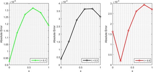
The numerical solutions of Test Problem (1) are reported in Tables 1 and 2. To prove the efficiency of the MVIA-II, comparison in terms of absolute errors is carried out the proposed technique and trigonometric B-spline collocation technique are reported in Table 1, while the comparison of MVIA-II and exact solutions are presented in Table 2. In comparison with [61] results, one can ensure that the results of MVIA-II are more accurate, efficient and reliable. Graphical results of Allen-Cahn equation corresponding Test Problem (1) are shown in Figures 1 and 2. In the first one, the behaviour of exact and MVIA-II solutions has been shown while in second the absolute errors graphs have been plotted for $t=0.001$ and $t=0.005$. It is cleared from figures that the MVIA-II can handle the nonlinear Parabolic equations precisely (Figure 3).

Figure 1. (Left): Behavior of exact and (Right): approximate solution for Test Problem 1.

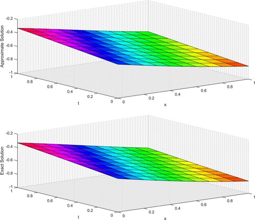
Figure 2. Comparing the curves of absolute errors for different time levels for Test Problem 1.

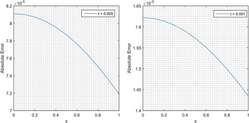
Figure 3. Comparing the curves of absolute errors for different time levels for the Test Problem 2.

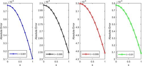
Table 1. Comparison in the form of absolute errors for Test Problem 1.

	$t=0.001$		$t=0.005$		$t=0.009$		$t=0.01$
$x$	Present	TBS [57]	Present	TBS [57]	Present	TBS [57]	Present	TBS [57]
0.1	1.620 E-05	2.448 E-04	8.101 E-05	9.687 E-04	1.454 E-04	1.492 E-03	1.621 E-04	1.606 E-03
0.2	1.614 E-05	2.000 E-04	8.073 E-05	1.016 E-03	1.445 E-04	1.761 E-03	1.615 E-04	1.935 E-03
0.3	1.604 E-05	1.797 E-04	8.024 E-05	9.082 E-04	1.433 E-04	1.644 E-03	1.606 E-04	1.826 E-03
0.4	1.590 E-05	1.594 E-04	7.956 E-05	8.052 E-04	1.418 E-04	1.465 E-03	1.593 E-04	1.632 E-03
0.5	1.572 E-05	1.410 E-04	7.869 E-05	7.124 E-04	1.399 E-04	1.296 E-03	1.576 E-04	1.444 E-03
0.6	1.551 E-05	1.242 E-04	7.764 E-05	6.280 E-04	1.378 E-04	1.143 E-03	1.555 E-04	1.273 E-03
0.7	1.526 E-05	1.091 E-04	7.643 E-05	5.520 E-04	1.353 E-04	1.003 E-03	1.531 E-04	1.116 E-03
0.8	1.499 E-05	9.502 E-05	7.505 E-05	4.824 E-04	1.326 E-04	8.536 E-04	1.504 E-04	9.434 E-04
0.9	1.468E-05	8.886 E-05	7.535 E-05	3.725 E-04	1.296 E-04	6.009 E-04	1.441E-04	6.534 E-04

Table 2. Comparison of the numerical results for Test Problem 1.

			Approximate solution		Absolute errors
$x$	$t$	Exact solution	Present	TBS [57]	Present
0.1	0.001	−0.48270191	−0.48268570	−0.48294667	1.620E−05
0.2	0.002	−0.46544517	−0.46541289	−0.46584916	3.228 E−05
0.3	0.003	−0.44827076	−0.448222628	−0.44881129	4.813 E−05
0.4	0.004	−0.43121885	−0.43115521	−0.43186126	6.363 E−05
0.5	0.005	−0.41432848	−0.41424978	−0.41504090	7.869 E−05
0.6	0.006	−0.39763717	−0.39754397	−0.39839276	9.320 E−05
0.7	0.007	−0.38118064	−0.38107357	−0.38195995	1.071 E−04
0.8	0.008	−0.36499250	−0.36487227	−0.36571227	1.202 E−04
0.9	0.009	−0.34910400	−0.34897140	−0.34910129	1.326 E−04

3.2. Test Problem 2 (Allen–Cahn equation)

Consider the Equation (1) with the values of constants as $n=3,\alpha =1\text{and}\text{β}=-1$, which gives the AC equation of the following form [57], (18) $\frac{\mathrm{\partial }v}{\mathrm{\partial }t}=\frac{{\mathrm{\partial }}^{2}v}{\mathrm{\partial }{x}^2}+v-v^3,$(18) Having the initial condition: $v\left(x,0\right)={\left(1+e^{-\frac{\sqrt{2}}{2}x}\right)}^{-1},$

And boundary conditions $\begin{array}{rl}v\left(0,t\right)& ={\left(1+e^{-\frac{3}{2}t}\right)}^{-1},\\ v\left(1,t\right)& ={\left(1+e^{-\frac{\sqrt{2}}{2}\left(1+\frac{3\sqrt{2}}{2}t\right)}\right)}^{-1},\end{array}$and exact solution from [57], which is: (19) $v\left(x,t\right)={\left(1+e^{-\frac{\sqrt{2}}{2}\left(x+\frac{3\sqrt{2}}{2}t\right)}\right)}^{-1}.$(19)

The relation of recurrence of VIM for Equation (18) is given by, (20) $\begin{array}{rl}{v}_{n+1}\left(x,t,h\right)& =v_n\left(x,t,h\right)+h{\int }_0^t\lambda \left(\varsigma \right)\\ & \times \left\{\frac{\mathrm{\partial }{v}_n\left(x,\varsigma ,h\right)}{\mathrm{\partial }\varsigma }-\stackrel{~}{\frac{{\mathrm{\partial }}^2{v}_n\left(x,\varsigma ,h\right)}{\mathrm{\partial }{x}^2}}\right.\\ & \left.-\widetilde{v_n\left(x,\varsigma ,h\right)}+\widetilde{v_n{\left(x,\varsigma ,h\right)}^3}\phantom{\frac{\mathrm{\partial }{v}_n\left(x,\varsigma ,h\right)}{\mathrm{\partial }\varsigma }}\right\}d\varsigma .\end{array}$(20) The value of $\lambda \left(\varsigma \right)$ can be obtained by the variational principle [58–60] or using the optimality condition, $\frac{\mathrm{\partial }{v}_{n+1}\left(x,t,h\right)}{\mathrm{\partial }{v}_n\left(x,t,h\right)}=0$We obtained the value of $\lambda \left(\varsigma \right)$, which is $\lambda \left(\varsigma \right)=-1$. By putting the value of $\lambda \left(\varsigma \right)$ in equation (20) gives (21) $\begin{array}{rl}{v}_{n+1}\left(x,t,h\right)& =v_n\left(x,t,h\right)-h{\int }_0^t\left\{\frac{\mathrm{\partial }{v}_n\left(x,\varsigma ,h\right)}{\mathrm{\partial }\varsigma }\right.\\ & -\frac{{\mathrm{\partial }}^2{v}_n\left(x,\varsigma ,h\right)}{\mathrm{\partial }{x}^2}-v_n\left(x,\varsigma ,h\right)\\ & \left.+v_n{\left(x,\varsigma ,h\right)}^3\phantom{\frac{{\mathrm{\partial }}^2{v}_n\left(x,\varsigma ,h\right)}{\mathrm{\partial }{x}^2}}\right\}d\varsigma .\end{array}$(21)

According to our proposed scheme (10), the following iterative formula is obtained (22) $\begin{array}{rl}{v}_{n+1}\left(x,t,h\right)& =v_0\left(x,t,h\right)+h{\int }_0^t\lambda \left(\varsigma \right)\left\{-\frac{{\mathrm{\partial }}^2{v}_n\left(x,\varsigma ,h\right)}{\mathrm{\partial }{x}^2}\right.\\ & \left.-v_n\left(x,\varsigma ,h\right)+v_n{\left(x,\varsigma ,h\right)}^3\phantom{\frac{{\mathrm{\partial }}^2{v}_n\left(x,\varsigma ,h\right)}{\mathrm{\partial }{x}^2}}\right\}d\varsigma ,\end{array}$(22)

We consider the initial approximation $v_0\left(x,t\right)$ as, $v_0\left(x,t\right)={\left(1+e^{-\frac{\sqrt{2}}{2}x}\right)}^{-1}.$Then from The relation of recurrence of VIM (22), we get the following other iterations, $\begin{array}{rl}{v}_1\left(x,t,h\right)& =\left(\text{exp}\right(\left(2^{\wedge }\right(1/2)\ast x)/2)\\ & \ast (2\ast \text{exp}(\left(2^{\wedge }\right(1/2)\ast x)/2)+3\ast h\ast t\\ & +2\left)\right)/(2\ast (\text{exp}\left(\right(2^{\wedge }\left(1/2\right)\ast x\left)/2\right)\\ & +1{)}^{\wedge }2),\end{array}$ $\begin{array}{rl}{v}_2\left(x,t,h\right)& =1/\left(\text{exp}\right(-\left(2^{\wedge }\right(1/2)\ast x)/2)+1)\\ & +(3\ast h\ast t\ast \text{exp}(\left(2^{\wedge }\right(1/2)\ast x)/2)\\ & \ast (96\ast \text{exp}(2^{\wedge }\left(1/2\right)\ast x)\\ & +16\ast \text{exp}(2\ast 2^{\wedge }(1/2)\ast x)\\ & +64\ast \text{exp}\left(\right(2^{\wedge }\left(1/2\right)\ast x\left)/2\right)\\ & +64\ast \text{exp((3}\ast 2^{\wedge }\ast x\left)/2\right)+12\ast h\ast t\\ & -24\ast h^{\wedge }2\ast t^{\wedge }2\ast \text{exp}\left(2^{\wedge }\right(1/2)\ast x)\\ & -9\ast h^{\wedge }3\ast t^{\wedge }3\ast \text{exp}\left(2^{\wedge }\right(1/2)\ast x)\\ & -24\ast h^{\wedge }2\ast t^{\wedge }2\ast \text{exp}\left(\right(3\ast 2^{\wedge }\left(1/2\right)\\ & \ast x\left)/2\right)-12\ast h\ast t\ast \text{exp}(2\ast 2^{\wedge }(1/2)\ast x)\\ & +24\ast h\ast t\ast \text{exp}\left(\right(2^{\wedge }\left(1/2\right)\ast x\left)/2\right)\\ & -24\ast h\ast t\ast \text{exp}\left(\right(3\ast 2^{\wedge }\left(1/2\right)\ast x\left)/2\right)\\ & +16\left)\right)/(32\ast (\text{exp}\left(\right(2^{\wedge }\left(1/2\right)\ast x\left)/2\right)\\ & +1{)}^{\wedge }6),\end{array}$ $⋮$ $⋮$ For obtained approximate solution $v_4\left(x,t,h\right)$, the following residual function can be used to find a valid value of h, (23) $\begin{array}{rl}{r}_4\left(x,t,h\right)& =\frac{\mathrm{\partial }{v}_4\left(x,t,h\right)}{\mathrm{\partial }t}-\frac{{\mathrm{\partial }}^2{v}_4\left(x,t,h\right)}{\mathrm{\partial }{x}^2}-v_4\left(x,t,h\right)\\ & +v_4(x,t,h{)}^2\end{array}$(23)

The norm 2 of residual function (23) with respect to $h$ for $\left(x,t\right)ϵ\left[0,1\right]\times \left[0,1\right]$ is: (24) $e_4\left(h\right)={\left[\frac{1}{{11}^2}\sum _{i=0}^{10}\sum _{j=0}^{10}{\left\{r_4\left(\frac{i}{10},\frac{j}{10},h\right)\right\}}^2\right]}^{\frac{1}{2}}$(24) The residual function (24) can be utilized for the approximation of $e_4\left(h\right)$ and an appropriate value of the $h$ can be found out by making the $e_4\left(h\right)$ minimum. The value of the auxiliary parameter is determined to 0.846053479477633 when the minimum value of $e_4\left(h\right)$ is 0.874216890183716032E-2. More precise and accurate results can be obtained when the number of iterations is increased. By means of this value of $h$ in $v_4\left(x,t,h\right)$ in the domain $\left(x,t\right)ϵ\left[0,1\right]\times \left[0,1\right]$, error b/w the exact and MVIA-II solutions can be seen in Figure 4, while the Comparison in the form of absolute errors of MVIA-II and TBS [42] for different values of $t$ are presented in Table 3.

Figure 4. Absolute error graph for x = 1 for Test Problem 3.

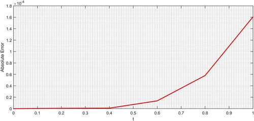
Table 3. Comparison of the numerical results for Test Problem 2.

	$t=0.001$		$t=0.005$		$t=0.009$		$t=0.01$
$x$	Present	TBS [57]	Present	TBS [57]	Present	TBS [57]	Present	TBS [57]
0.1	3.765 E-05	2.509 E-04	2.882 E-04	1.127 E-03	5.187 E-04	1.917 E-03	5.763 E-04	2.108 E-03
0.2	5.744 E-05	3.351 E-04	2.871 E-04	1.715 E-03	5.165 E-04	3.100 E-03	5.738 E-04	3.446 E-03
0.3	5.708 E-05	4.389 E-04	2.852 E-04	2.233 E-03	5.131 E-04	4.085 E-03	5.700E-04	4.555 E-03
0.4	5.658 E-05	5.456 E-04	2.827 E-04	2.768 E-03	5.084 E-04	5.057 E-03	5.648 E-04	5.639 E-03
0.5	5.595 E-05	6.542 E-04	2.795 E-04	3.314 E-03	5.025 E-04	6.042 E-03	5.582 E-04	6.735 E-03
0.6	5.519 E-05	7.626 E-04	2.756 E-04	3.857 E-03	4.956 E-04	7.028 E-03	5.505 E-04	7.830 E-03
0.7	5.432 E-05	8.697 E-04	2.712 E-04	4.399 E-03	4.875 E-04	7.968 E-03	5.415 E-04	8.850 E-03
0.8	5.333 E-05	9.653 E-04	2.662 E-04	4.902 E-03	4.785 E-04	8.510 E-03	5.314 E-04	9.353 E-03
0.9	5.224 E-05	1.161 E-03	2.607 E-04	4.617 E-03	4.685 E-04	7.136 E-03	5.203 E-04	7.685 E-03

Table 4. Comparison of the numerical results for Test Problem 3.

			Approximate solution		Absolute errors
$t$	$x$	Exact Solution	Present	VIM [62]	Present	VIM [62]
0	1	0.159466223943033	0.159466223943033	0.1594662239430331	2.498E−16	0
0.2	1	0.193509037431178	0.193509600917448	0.1935090374311784	5.635E−07	2.1E−06
0.4	1	0.231630452841077	0.231629619298055	0.2316304528410767	8.335E−07	5.3E−05
0.6	1	0.273447260416673	0.273433638969862	0.2734472604166732	1.362E−05	3.2E−04
0.8	1	0.318375189312876	0.318317204172162	0.3183751893128759	5.799E−05	1.1E−02
1	1	0.365661380536344	0.365500671580091	0.3656613805363442	1.607E−04	2.6E−02

3.3. Test Problem 3 (Newell–Whitehead equation)

Consider the Equation (1) with the values of constants as $n=2,\alpha =1\text{and}\text{β}=-1$, which gives the NW equation of the following form (25) $\frac{\mathrm{\partial }v}{\mathrm{\partial }t}=\frac{{\mathrm{\partial }}^{2}v}{\mathrm{\partial }{x}^2}+v-v^2,$(25) having initial condition: $v\left(x,0\right)={\left(1+e^{\frac{x}{\sqrt{6}}}\right)}^{-2}$

and exact solution from [62], which is: (26) $v\left(x,t\right)={\left(1+e^{\frac{x}{\sqrt{6}}-\frac{5}{6}t}\right)}^{-2}.$(26)

By applying MVIA-I, The relation of recurrence of VIM for Equation (25) is given by, (27) $\begin{array}{rl}{v}_{n+1}\left(x,t,h\right)& =v_n\left(x,t,h\right)+h{\int }_0^t\lambda \left(\varsigma \right)\left\{\frac{\mathrm{\partial }{v}_n\left(x,\varsigma ,h\right)}{\mathrm{\partial }\varsigma }\right.\\ & -\stackrel{~}{\frac{{\mathrm{\partial }}^2{v}_n\left(x,\varsigma ,h\right)}{\mathrm{\partial }{x}^2}}-\widetilde{v_n\left(x,\varsigma ,h\right)}\\ & \left.+\widetilde{v_n{\left(x,\varsigma ,h\right)}^2}\right\}d\varsigma ,\end{array}$(27) The value of $\lambda \left(\varsigma \right)$ can be obtained by the variational principle [58–60] or using the optimality condition, $\frac{\mathrm{\partial }{v}_{n+1}\left(x,t,h\right)}{\mathrm{\partial }{v}_n\left(x,t,h\right)}=0$We obtained the value of $\lambda \left(\varsigma \right)$, which is $\lambda \left(\varsigma \right)=-1$. By putting the value of $\lambda \left(\varsigma \right)$ in equation (27) gives in the following iterative structure: (28) $\begin{array}{rl}{v}_{n+1}\left(x,t,h\right)& =v_n\left(x,t,h\right)-h{\int }_0^t\left\{\frac{\mathrm{\partial }{v}_n\left(x,\varsigma ,h\right)}{\mathrm{\partial }\varsigma }\right.\\ & -\frac{{\mathrm{\partial }}^2{v}_n\left(x,\varsigma ,h\right)}{\mathrm{\partial }{x}^2}-v_n\left(x,\varsigma ,h\right)\\ & +\left.v_n{\left(x,\varsigma ,h\right)}^2\phantom{\frac{{\mathrm{\partial }}^2{v}_n\left(x,\varsigma ,h\right)}{\mathrm{\partial }{x}^2}}\right\}d\varsigma .\end{array}$(28) According to our proposed scheme (10), the following iterative formula is obtained (29) $\begin{array}{rl}{v}_{n+1}\left(x,t,h\right)& =v_0\left(x,t,h\right)+h{\int }_0^t\lambda \left(\varsigma \right)\left\{-\frac{{\mathrm{\partial }}^2{v}_n\left(x,\varsigma ,h\right)}{\mathrm{\partial }{x}^2}\right.\\ & \left.-v_n\left(x,\varsigma ,h\right)+v_n{\left(x,\varsigma ,h\right)}^2\phantom{\frac{{\mathrm{\partial }}^2{v}_n\left(x,\varsigma ,h\right)}{\mathrm{\partial }{x}^2}}\right\}d\varsigma ,\end{array}$(29) We consider the initial approximation $v_0\left(x,t\right)$ as, $v_0\left(x,t\right)=\frac{1}{{\left(1+e^{\frac{x}{\sqrt{6}}}\right)}^2}.$Then from The relation of recurrence of VIM (29), we get the following other iterations, $\begin{array}{rl}{v}_1\left(x,t,h\right)& =(3\ast exp(\left(6^{\wedge }\left(1/2\right)\ast x\right)/6)+5\ast h\ast t\\ & \ast exp\left(\left(6^{\wedge }\left(1/2\right)\ast x\right)/6\right)+3)/\\ & \times \left(3\ast (exp\left(\left(6^{\wedge }\left(1/2\right)\ast x\right)/6\right)+1{)}^{\wedge }3\right),\end{array}$ $\begin{array}{rl}{v}_2(x,t,h)& =1/\left(\text{exp}\right(\left(6^{\wedge }\right(1/2)\ast x)/6)+1{)}^{\wedge }2\\ & +(h\ast ((5\ast t\ast \text{exp}(\left(6^{\wedge }\right(1/2)\ast x)/6)\\ & \ast (36\ast \text{exp}(\left(6^{\wedge }\right(1/2)\ast x)/2)\\ & +108\ast \text{exp}\left(\right(6^{\wedge }\left(1/2\right)\ast x\left)/3\right)\\ & -15\ast h\ast t+30\ast h\ast t\ast \text{exp}\left(\right(6^{\wedge }\left(1/2\right)\\ & \ast x\left)/2\right)+45\ast h\ast t\ast \text{exp}\left(\right(6^{\wedge }\left(1/2\right)\\ & \ast x\left)/3\right)+36\left)\right)/108-(5\ast t\ast \text{exp}((6^{\wedge }\\ & \times \left(1/2\right)\ast x\left)/3\right)\ast (20\ast h^{\wedge }2\ast t^{\wedge }2\\ & -108\left)\right)/108\left)\right)/\left(\text{exp}\right(\left(6^{\wedge }\right(1/2)\ast x)/6)\\ & +1{)}^{\wedge }6,\end{array}$ $⋮$ $⋮$

For obtained approximate solution $v_4\left(x,t,h\right)$, the following residual function can be used to find a valid value of h, (30) $\begin{array}{rl}{r}_4\left(x,t,h\right)& =\frac{\mathrm{\partial }{v}_4\left(x,t,h\right)}{\mathrm{\partial }t}-\frac{{\mathrm{\partial }}^2{v}_4\left(x,t,h\right)}{\mathrm{\partial }{x}^2}-v_4\left(x,t,h\right)\\ & +v_4(x,t,h{)}^2\end{array}$(30)

The norm 2 of residual function (30) with respect to $h$ for $\left(x,t\right)ϵ\left[0,1\right]\times \left[0,1\right]$ is: (31) $e_4\left(h\right)={\left[\frac{1}{{11}^2}\sum _{i=0}^{10}\sum _{j=0}^{10}{\left\{r_4\left(\frac{i}{10},\frac{j}{10},h\right)\right\}}^2\right]}^{\frac{1}{2}}$(31) The residual function (31) can be utilized for the approximation of $e_4\left(h\right)$ and an appropriate value of the $h$ can be found out by making the $e_4\left(h\right)$ minimum. The value of the auxiliary parameter is determined to be1.00001765132560 when the minimum value of $e_4\left(h\right)$ is achieved. More precise and accurate results can be obtained when the number of iterations is increased. By means of this value of $h$ in $v_4\left(x,t,h\right)$ in the domain $\left(x,t\right)ϵ\left[0,1\right]\times \left[0,1\right]$, error b/w the exact and MVIA-II solutions can be seen in Figure 4, while the comparison of MVIA-II and exact solutions, as well as Comparison in the form of absolute errors with VIM, is presented in Table 4, which show that the proposed technique can handle the Newell–Whitehead equations precisely.

Table 5. Comparison of the numerical results for Test Problem 4.

	$t=0.1$		$t=0.3$		$t=0.5$
$x$	Present	HPTM [63]	Present	HPTM [63]	Present	HPTM [63]
0.1	9.2588440E-06	1.221229E-4	3.8573053E-05	3.022038E-3	16215066 E-03	1.245533E-2
0.2	1.1350216E-05	1.328287E-4	1.5193154 E-04	3.415236E-3	1.8704859 E-04	1.462723E-2
0.4	1.2689898E-05	1.352957E-4	2.9185887E-04	3.602846E-3	1.6733416E-03	1.597269E-2
0.6	1.3157393E-05	1.296021E-4	3.6312075E-04	3.570756E-3	2.6144372 E-03	1.636664E-2
0.8	1.2819577E-05	1.168616E-4	3.6523601E-04	3.333532E-3	2.9338374 E-03	1.580592E-2
1.0	11888620E-05	9.893015E-5	3.1331675E-04	2.929772E-3	2.7080923 E-03	1.440339E-2

3.4. Test Problem 4 (Newell–Whitehead equation)

Consider the Equation (1) with the values of constants as $n=4,\alpha =1\text{and}\text{β}=-1$, which gives the NW equation of the following form the [63] (32) $\frac{\mathrm{\partial }v}{\mathrm{\partial }t}=\frac{{\mathrm{\partial }}^{2}v}{\mathrm{\partial }{x}^2}+v-v^4,0<x<1,t>0,$(32) having the initial condition: $v\left(x,0\right)={\left(1+e^{\frac{3x}{\sqrt{10}}}\right)}^{-\frac{2}{3}},$and exact solution from [63], which is: (33) $v\left(x,t\right)={\left[\frac{1}{2}\text{tan}h\left\{-\frac{3}{2\sqrt{10}}\left(x-\frac{7}{\sqrt{10}}t\right)\right\}+\frac{1}{2}\right]}^{\frac{2}{3}}$(33)

The relation of recurrence of VIM for Equation (32) is given by, (34) $\begin{array}{rl}{v}_{n+1}\left(x,t,h\right)& =v_n\left(x,t,h\right)+h{\int }_0^t\lambda \left(\varsigma \right)\left\{\phantom{\frac{{\mathrm{\partial }}^2{v}_n\left(x,\varsigma ,h\right)}{\mathrm{\partial }{x}^2}}\frac{\mathrm{\partial }{v}_n\left(x,\varsigma ,h\right)}{\mathrm{\partial }\varsigma }\right.\\ & -\stackrel{~}{\frac{{\mathrm{\partial }}^2{v}_n\left(x,\varsigma ,h\right)}{\mathrm{\partial }{x}^2}}-\widetilde{v_n\left(x,\varsigma ,h\right)}\\ & \left.+\widetilde{v_n{\left(x,\varsigma ,h\right)}^4}\phantom{\frac{{\mathrm{\partial }}^2{v}_n\left(x,\varsigma ,h\right)}{\mathrm{\partial }{x}^2}}\right\}d\varsigma ,\end{array}$(34)

The value of $\lambda \left(\varsigma \right)$ can be obtained by the variational principle [58–60] or using the optimality condition, $\frac{\mathrm{\partial }{v}_{n+1}\left(x,t,h\right)}{\mathrm{\partial }{v}_n\left(x,t,h\right)}=0$We obtained the value of $\lambda \left(\varsigma \right)$, which is $\lambda \left(\varsigma \right)=-1$. By putting the value of $\lambda \left(\varsigma \right)$ in equation (34) gives in the following iterative structure: (35) $\begin{array}{rl}{v}_{n+1}\left(x,t,h\right)& =v_n\left(x,t,h\right)-h{\int }_0^t\\ & \times \left\{\frac{\mathrm{\partial }{v}_n\left(x,\varsigma ,h\right)}{\mathrm{\partial }\varsigma }-\frac{{\mathrm{\partial }}^2{v}_n\left(x,\varsigma ,h\right)}{\mathrm{\partial }{x}^2}\right.\\ & \left.-v_n\left(x,\varsigma ,h\right)+v_n{\left(x,\varsigma ,h\right)}^4\phantom{\frac{{\mathrm{\partial }}^2{v}_n\left(x,\varsigma ,h\right)}{\mathrm{\partial }{x}^2}}\right\}d\varsigma ,\end{array}$(35)

According to our proposed scheme (10), the following iterative formula is obtained (36) $\begin{array}{rl}{v}_{n+1}\left(x,t,h\right)& =v_0\left(x,t,h\right)+h{\int }_0^t\lambda \left(\varsigma \right)\\ & \times \left\{-\frac{{\mathrm{\partial }}^2{v}_n\left(x,\varsigma ,h\right)}{\mathrm{\partial }{x}^2}-v_n\left(x,\varsigma ,h\right)\right.\\ & \left.+v_n{\left(x,\varsigma ,h\right)}^2)\phantom{\frac{{\mathrm{\partial }}^2{v}_n\left(x,\varsigma ,h\right)}{\mathrm{\partial }{x}^2}}\right\}d\varsigma ,\end{array}$(36)

We consider the initial approximation $v_0\left(x,t\right)$ as, $v_0\left(x,t\right)={\left(1+e^{\frac{3x}{\sqrt{10}}}\right)}^{\frac{-2}{3}},$Then from The relation of recurrence of VIM (36), we get the following other iterations, $\begin{array}{rl}{v}_1\left(x,t,h\right)& =\left(\right(1/\left(\text{exp}\right((3\ast {10}^{\wedge }(1/2)\ast x)/10)+1){)}^{\wedge }\\ & \times \left(5/3\right)\ast (5\ast \text{exp}((3\ast {10}^{\wedge }(1/2)\ast x)/10)\\ & +7\ast h\ast t\ast \text{exp}\left(\right(3\ast {10}^{\wedge }\left(1/2\right)\ast x\left)/10\right)\\ & +5\left)\right)/5,\end{array}$ $⋮$ $⋮$

For obtained approximate solution, the following residual function can be used to find a valid value of h (37) $\begin{array}{rl}{r}_4\left(x,t,h\right)& =\frac{\mathrm{\partial }{v}_4\left(x,t,h\right)}{\mathrm{\partial }t}-\frac{{\mathrm{\partial }}^2{v}_4\left(x,t,h\right)}{\mathrm{\partial }{x}^2}-v_4\left(x,t,h\right)\\ & +v_4(x,t,h{)}^4\end{array}$(37)

The norm 2 of residual function (37) for 4th-order approximation with respect to $h$ for $\left(x,t\right)ϵ\left[0,1\right]\times \left[0,1\right]$ is (38) $e_4\left(h\right)={\left[\frac{1}{{11}^2}\sum _{i=0}^{10}\sum _{j=0}^{10}{\left\{r_4\left(\frac{i}{10},\frac{j}{10},h\right)\right\}}^2\right]}^{\frac{1}{2}}$(38)

The residual function (38) can be utilized for the approximation of $e_4\left(h\right)$ and an appropriate value of the $h$ can be found out by making the $e_4\left(h\right)$ minimum. The value of the auxiliary parameter is determined to be 0.999795976281803 when the minimum value of $e_4\left(h\right)$ is 0.347702197150023600e-3. More precise and accurate results can be obtained when the number of iterations is increased.

Utilizing the value of $h$ in $v_4\left(x,t,h\right)$ in the domain $\left(x,t\right)ϵ\left[0,1\right]\times \left[0,1\right]$, the comparison of exact and MVIA-II solutions can be seen in Figure 5 for different values of $t$, while to prove the effectiveness of the suggested technique for various values of $t,x$ and absolute errors in Table 5 along with the results of homotopy perturbation transform technique given in [63]. One can ensure that the results of MVIA-II are more accurate and can be obtained in a very short time.

Figure 5. Comparing the curves of absolute errors for different time levels for the Test Problem 4.

3.5. Test Problem 5 (Fisher equation)

Consider the Equation (1) with the values of constants as $n=2,\alpha =6\text{and}\text{β}=-6$, which gives the Fisher equation of the form [64], (39) $\frac{\mathrm{\partial }v}{\mathrm{\partial }t}=\frac{{\mathrm{\partial }}^{2}v}{\mathrm{\partial }{x}^2}+6v\left(1-v\right),$(39) having the initial condition: $v\left(x,0\right)=(1+e^x{)}^{-2},$And exact solution from [64], which is: (40) $v\left(x,t\right)=(1+e^{x-5t}{)}^{-2}.$(40)

The relation of recurrence of VIM for Equation (39) is given by, (41) $\begin{array}{rl}{v}_{n+1}\left(x,t,h\right)& =v_n\left(x,t,h\right)+h{\int }_0^t\lambda \left(\varsigma \right)\left\{\frac{\mathrm{\partial }{v}_n\left(x,\varsigma ,h\right)}{\mathrm{\partial }\varsigma }\right.\\ & -\stackrel{~}{\frac{{\mathrm{\partial }}^2{v}_n\left(x,\varsigma ,h\right)}{\mathrm{\partial }{x}^2}}-6\widetilde{v_n}\left(x,\varsigma ,h\right)\\ & \times \left.\left(\widetilde{1-v_n}\left(x,\varsigma ,h\right)\right)\phantom{\frac{\mathrm{\partial }{v}_n\left(x,\varsigma ,h\right)}{\mathrm{\partial }\varsigma }}\right\}d\varsigma ,\end{array}$(41)

The value of $\lambda \left(\varsigma \right)$ can be obtained by the variational principle [58–60] or using the optimality condition, $\frac{\mathrm{\partial }{v}_{n+1}\left(x,t,h\right)}{\mathrm{\partial }{v}_n\left(x,t,h\right)}=0$We obtained the value of $\lambda \left(\varsigma \right),$ which is $\lambda \left(\varsigma \right)=-1.$ By putting value of $\lambda \left(\varsigma \right)$ in equation (39) gives (42) $\begin{array}{rl}{v}_{n+1}\left(x,t,h\right)& =v_0\left(x,t,h\right)+h{\int }_0^t\lambda \left(\varsigma \right)\left\{-\frac{{\mathrm{\partial }}^2{v}_n\left(x,\varsigma ,h\right)}{\mathrm{\partial }{x}^2}\right.\\ & \left.-6v_n\left(x,\varsigma ,h\right)\left(1-v_n\left(x,\varsigma ,h\right)\right)\phantom{\frac{{\mathrm{\partial }}^2{v}_n\left(x,\varsigma ,h\right)}{\mathrm{\partial }{x}^2}}\right\}d\varsigma ,\end{array}$(42) According to our proposed scheme (10), the following iterative formula is gained (43) $\begin{array}{rl}{v}_{n+1}\left(x,t,h\right)& =v_0\left(x,t,h\right)+h{\int }_0^t\lambda \left(\varsigma \right)\\ & \times \left\{-\frac{{\mathrm{\partial }}^2{v}_n\left(x,\varsigma ,h\right)}{\mathrm{\partial }{x}^2}-v_n\left(x,\varsigma ,h\right)\right.\\ & \left.\times \left(1-v_n{\left(x,\varsigma ,h\right)}^2\right)\phantom{\frac{{\mathrm{\partial }}^2{v}_n\left(x,\varsigma ,h\right)}{\mathrm{\partial }{x}^2}}\right\}d\varsigma ,\end{array}$(43) We consider the initial approximation $v_0\left(x,t\right)$ as, $v_0\left(x,t\right)=(1+e^x{)}^{-2},$Then from The relation of recurrence of VIM (43), we get the following other iterations, $\begin{array}{rl}{v}_1\left(x,t,h\right)& =\left(exp\left(x\right)+10\ast h\ast t\ast exp\left(x\right)+1\right)/\\ & \times (exp\left(x\right)+1{)}^{\wedge }3,\end{array}$ $\begin{array}{rl}{v}_2\left(x,t,h\right)& =1/\left(\text{exp}\right(x)+1{)}^{\wedge }2-(h\ast (5\ast t\ast \text{exp}\\ & \times (2\ast x)\ast (40\ast h^{\wedge }2\ast t^{\wedge }2-6)\\ & -5\ast t\ast \text{exp}\left(x\right)\ast (6\ast \text{exp}(2\ast x)\\ & +2\ast \text{exp}(3\ast x)-5\ast h\ast t+15\ast h\ast t\\ & \ast \text{exp}(2\ast x)+10\ast h\ast t\ast \text{exp}(3\ast x)+2\left)\right))\\ & /\left(\text{exp}\right(x)+1{)}^{\wedge }6,\end{array}$ $⋮$ $⋮$ For obtained approximate solution, the following residual function can be used to find a valid value of h (44) $\begin{array}{rl}{r}_3\left(x,t,h\right)& =\frac{\mathrm{\partial }{v}_3\left(x,t,h\right)}{\mathrm{\partial }t}-\frac{{\mathrm{\partial }}^2{v}_3\left(x,t,h\right)}{\mathrm{\partial }{x}^2}\\ & -6v_3\left(x,t,h\right)\left(1-v_3\left(x,\varsigma ,h\right)\right).\end{array}$(44) The norm 2 of residual function (44) for 3rd-order approximation with respect to $h$ for $\left(x,t\right)ϵ\left[0,1\right]\times \left[0,1\right]$ is (45) $e_3\left(h\right)={\left[\frac{1}{{\left(11\right)}^2}\sum _{i=0}^{10}\sum _{j=0}^{10}{\left\{r_3\left(\frac{i}{10},\frac{j}{10},h\right)\right\}}^2\right]}^{\frac{1}{2}}$(45) The residual function (45) can be utilized for the approximation of $e_3\left(h\right)$ and an appropriate value of the $h$ can be found out by making the $e_3\left(h\right)$ minimum. The value of the auxiliary parameter is determined to be 0.971647912904180 when the minimum value of $e_3\left(h\right)$ is obtained which is 0.617775361521317526e-1. More precise and accurate results can be obtained when the number of iterations is increased. Utilizing the value of $h$ in $v_3\left(x,t,h\right)$ in the domain $\left(x,t\right)ϵ\left[0,1\right]\times \left[0,1\right]$, the following results are obtained.

Comparison of results of the MVIA-II with the results produced by approaches reported in [64] is shown in Table 5, which demonstrate that the overall results of proposed MVIA-II are either better or same with the results of [64], where modified variational iteration method and Adomian decomposition method are employed. In Figure 6, the absolute error graphs are plotted for $t=0.2$, $t=0.3$ and $t=0.4$. It is cleared from figure and table that the proposed MVIA-II can handle the fisher equation accurately.

Figure 6. Absolute error graph for different times for Test Problem 6.

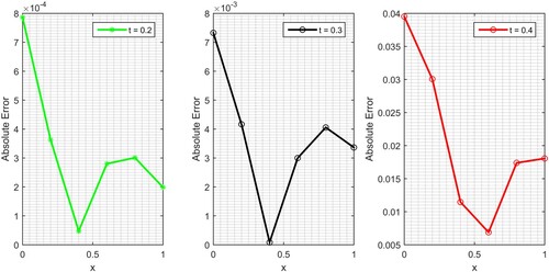
Table 6. Comparison in the form of absolute errors for Test Problem 6.

	$t=0.2$			$t=0.4$
$x$	Present	ADM [64]	MVIM [64]	Present	ADM [64]	MVIM [64]
0	7.8637525 E-04	7.22002 E-03	2.69962 E-03	3.9521338 E-02	5.75298 E-02	5.01844 E-02
0.2	3.6257440 E-04	9.89049 E-03	2.15566 E-03	3.0056850 E-02	1.6115 E-01	5.27127 E-02
0.4	4.7452743 E-05	1.09765 E-02	1.136097 E-03	1.1467670 E-02	1.39113 E-01	4.12072 E-02
0.6	2.7987518 E-04	1.04039 E-02	7.38299 E-04	6.8928130 E-03	1.51579 E-01	2.25459 E-02
0.8	3.0106076 E-04	8.50732 E-03	5.73101 E-04	1.73835851 E-02	1.43529 E-01	5.28693 E-03
1.0	1.9885243 E-04	5.87222 E-03	9.07727 E-04	1.8052646 E-02	1.19333 E-01	4.23672 E-03

4. Conclusions

In this article, we have studied and analyzed an iterative algorithm named as modified variational iteration algorithm-II for solving Allen–Cahn, Newell–Whitehead and Fisher equations with different parameters and presented in great detail, including tabulated numerical results and figures. This modified algorithm makes simple the computational work and results of high degree precision can be gotten in limited iterations as compared to other known approaches like variational iteration method, trigonometric B-spline collocation method, homotopy perturbation transform method, modified variational iteration method and Adomian decomposition method.

The proposed method will be able to use without using discretization, shape parameter, Adomian polynomials, transformation, linearization or restrictive assumptions and thus are particularly perfect with the expanded and flexible nature of the physical problems. Furthermore, the modification based upon the auxiliary parameter is easier to use and is more user friendly. The main advantage is that the auxiliary parameter involved in the MVIA-II is able to control the convergence rate and its optimum value can be determined.

Hence, we infer that the proposed algorithm is a reliable and proficient incredible scientific instrument for tackling nonlinear Parabolic problems in science and engineering.

Disclosure statement

No potential conflict of interest was reported by the author(s).

References

- Ismail HNA, Raslan K, Abd Rabboh AA. Adomian decomposition method for Burger’s–Huxley and Burger’s–Fisher equations. Appl Math Comput. 2004;159(1):291–301.
- Patil HM, Maniyeri R. Finite difference method based analysis of bio-heat transfer in human breast cyst. Therm Sci Eng Prog. 2019;10:42–47.
- Kheiri H, Alipour N, Dehghani R. Homotopy analysis and Homotopy-Pade methods for the modified Burgers-Korteweg-de-Vries and the Newell Whitehead equation. Math Sci. 2011;5(1):33–50.
- He J-H. Variational principle for the generalized KdV-Burgers equation with fractal derivatives for shallow water waves. J Appl Comput Mech. 2020;6(4):735–740.
- Zayed EME, Alurrfi KAE. A new Jacobi elliptic function expansion method for solving a nonlinear PDE describing the nonlinear low-pass electrical lines. Chaos Solitons Fractals. 2015;78:148–155.
- Yang J, Tang T, Song H, et al. Nonlinear stability of the implicit-explicit methods for the Allen-Cahn equation. Inverse Probl Imaging. 2013;7(3):679–695.
- Wazwaz A-M. The tanh–coth method for solitons and kink solutions for nonlinear parabolic equations. Appl Math Comput. 2007;188(2):1467–1475.
- Babolian E, Saeidian J. Analytic approximate solutions to Burgers, Fisher, Huxley equations and two combined forms of these equations. Commun Nonlinear Sci Numer Simul. 2009;14(5):1984–1992.
- Ji B, Zhang L. Error estimates of exponential wave integrator Fourier pseudospectral methods for the nonlinear Schrödinger equation. Appl Math Comput. 2019;343:100–113.
- Wazwaz A-M. The Hirota’s bilinear method and the tanh–coth method for multiple-soliton solutions of the Sawada–Kotera–Kadomtsev–Petviashvili equation. Appl Math Comput. 2008;200(1):160–166.
- Patra A, Saha Ray S. Homotopy perturbation sumudu transform method for solving convective radial fins with temperature-dependent thermal conductivity of fractional order energy balance equation. Int J Heat Mass Transf. 2014;76:162–170.
- Costa R, Nóbrega JM, Clain S, et al. Very high-order accurate finite volume scheme for the convection-diffusion equation with general boundary conditions on arbitrary curved boundaries. Int J Numer Methods Eng. 2019;117(2):188–220.
- Safdari Shadloo M. Numerical simulation of compressible flows by lattice Boltzmann method. Numer Heat Transf Part A Appl. 2019;75(3):167–182.
- Nur Alam M, Ali Akbar M. Some new exact traveling wave solutions to the simplified MCH equation and the (1+1)-dimensional combined KdV-mKdV equations. J Assoc Arab Univ Basic Appl Sci. 2015;17:6–13.
- Alam MN. Exact solutions to the foam drainage equation by using the new generalized (G’/G)-expansion method. Results Phys. 2015;5:168–177.
- Rafiq M, Ahmad H, Mohyud-Din ST. Variational iteration method with an auxiliary parameter for solving Volterra’s population model. Nonlinear Sci. 2018;4:835–839.
- Hariharan G, Kannan K. Haar wavelet method for solving some nonlinear parabolic equations. J Math Chem. 2010;48(4):1044–1061.
- Hariharan G. An efficient Legendre wavelet-based approximation method for a few Newell–Whitehead and Allen–Cahn equations. J Membr Biol. 2014;247(5):371–380.
- Yokus A, Bulut H. On the numerical investigations to the Cahn-Allen equation by using finite difference method. An Int J Optim Control Theor Appl. 2018;9(1):18.
- Bulut H, Atas SS, Baskonus HM. Some novel exponential function structures to the Cahn-Allen equation. Cogent Phys. 2016;3(1).
- Gui C, Zhao M. Traveling wave solutions of Allen–Cahn equation with a fractional Laplacian. Ann l’Institut Henri Poincare Non Linear Anal. 2015;32(4):785–812.
- Jeong D, Kim J. An explicit hybrid finite difference scheme for the Allen–Cahn equation. J Comput Appl Math. 2018;340:247–255.
- Niu J, Xu M, Yao G. An efficient reproducing kernel method for solving the Allen–Cahn equation. Appl Math Lett. 2019;89:78–84.
- Chen Y, Huang Y, Yi N. Recovery type a posteriori error estimation of adaptive finite element method for Allen–Cahn equation. J Comput Appl Math. 2019;361: 112574.
- Ezzati R, Shakibi K. Using adomian’s decomposition and multiquadric quasi-interpolation methods for solving Newell–Whitehead equation. Procedia Comput Sci. 2011;3:1043–1048.
- Sakaguchi H. Zigzag instability and reorientation of roll pattern in the Newell-Whitehead equation. Prog Theor Phys. 1991;86(4):759–763.
- Antoniou SM. The Riccati equation method with variable expansion coefficients. III. Solving the Newell-Whitehead equation. Differ Equations Appl. 2009;369(1):93–132.
- Fisher RA. The wave of advance of advantageous genes. Ann Eugen. 1937;7(4):355–369.
- Frank-Kamenetskii DA. Diffusion and heat exchange in chemical kinetics. Oxford: Princeton University Press; 2016.
- Tuckwell HC. Introduction to theoretical neurobiology. Cambridge: Cambridge University Press; 1988.
- Brazhnik PK, Tyson JJ. On traveling wave solutions of Fisher’s equation in two spatial dimensions. SIAM J Appl Math. 2000;60(2):371–391.
- Hariharan G, Kannan K, Sharma KR. Haar wavelet method for solving Fisher’s equation. Appl Math Comput. 2009;211(2):284–292.
- Zhang R, Yu X, Zhao G. The local discontinuous Galerkin method for Burger’s–Huxley and Burger’s–Fisher equations. Appl Math Comput. 2012;218(17):8773–8778.
- Moghimi M, Hejazi FSA. Variational iteration method for solving generalized Burger–Fisher and Burger equations. Chaos Solitons Fractals. 2007;33(5):1756–1761.
- Javidi M. Modified pseudospectral method for generalized Burger’s-Fisher equation. Int Math Forum. 2006;1(29–32):1555–1564.
- Triki H, Wazwaz A-M. Trial equation method for solving the generalized Fisher equation with variable coefficients. Phys Lett A. 2016;380(13):1260–1262.
- Wazwaz A-M, Gorguis A. An analytic study of Fisher’s equation by using Adomian decomposition method. Appl Math Comput. 2004;154(3):609–620.
- Ahmad H, Khan TA. Variational iteration algorithm-I with an auxiliary parameter for wave-like vibration equations. J Low Freq Noise Vib Act Control. 2019;38(3–4):1113–1124.
- Ahmad H, Khan TA, Cesarano C. Numerical solutions of coupled Burgers’ equations. Axioms. 2019;8(4):119.
- Ahmad H, Seadawy AR, Khan TA. Numerical solution of Korteweg-de Vries-Burgers equation by the modified variational iteration algorithm-II arising in shallow water waves. Physica Scripta. 2020;95:045210.
- Ahmad H. Auxiliary parameter in the variational iteration algorithm-II and its optimal determination. Nonlinear Sci Lett A. 2018;9(1):62–72.
- Nadeem M, Li F, Ahmad H. Modified Laplace variational iteration method for solving fourth-order parabolic partial differential equation with variable coefficients. Comput Math Appl. 2019;87:2025.
- Seadawy AR, Lu D, Yue C. Travelling wave solutions of the generalized nonlinear fifth-order KdV water wave equations and its stability. Journal of Taibah University for Science. 2017;11:623–633.
- Seadawy AR, Alamri SZ. Mathematical methods via the nonlinear two-dimensional water waves of Olver dynamical equation and its exact solitary wave solutions. Results Phys. 2018;8:286–291.
- Seadawy AR, Iqbal M, Lu D. Nonlinear wave solutions of the Kudryashov–Sinelshchikov dynamical equation in mixtures liquid-gas bubbles under the consideration of heat transfer and viscosity. J Taibah Univ Sci. 2019;13(1):1060–1072.
- Seadawy AR, El-Rashidy K. Dispersive solitary wave solutions of Kadomtsev-Petviashvili and modified Kadomtsev-Petviashvili dynamical equations in unmagnetized dust plasma. Results Phys. 2018;8:1216–1222.
- Seadawy AR, Manafian J. New soliton solution to the longitudinal wave equation in a magneto-electro-elastic circular rod. Results Phys. 2018;8:1158–1167.
- Alam MN, Alam MM. An analytical method for solving exact solutions of a nonlinear evolution equation describing the dynamics of ionic currents along microtubules. J Taibah Univ Sci. 2017;11(6):939–948.
- Seadawy AR. Three-dimensional weakly nonlinear shallow water waves regime and its traveling wave solutions. Int J Comput Methods. 2018;15(3):1850017.
- Alam MN, Tunc C. An analytical method for solving exact solutions of the nonlinear Bogoyavlenskii equation and the nonlinear diffusive predator-prey system. Alexandria Eng J. 2016;55(2):1855–1865.
- Alam MN, Li X. Exact traveling wave solutions to higher order nonlinear equations. J Ocean Eng Sci. 2019;4(3):276–288.
- Nur Alam M, Hafez MG, Ali Akbar M, et al. Exact traveling wave solutions to the (3+1)-dimensional mKdV-ZK and the (2+1)-dimensional Burgers equations via exp(-Φ(η))-expansion method. Alexandria Eng J. 2015;54(3):635–644.
- Seadawy AR. Solitary wave solutions of tow-dimensional nonlinear Kadomtsev-Petviashvili dynamic equation in a dust acoustic plasmas. Pramana. 2017;89:1–11, article no. 49.
- Inokuti M, Sekine H, Mura T. General use of the Lagrange multiplier in nonlinear mathematical physics. Oxford: Pergamon Press; 1978.
- He J-H, Wu G-C, Austin F. The variational iteration method which should be followed. Nonlinear Sci Lett A. 2010;1(1):1–30.
- He J-H, Wu X-H. Variational iteration method: New development and applications. Comput Math Appl. 2007;54(7–8):881–894.
- Zahra WK. Trigonometric B-spline collocation method for solving PHI-four and Allen–Cahn equations. Mediterr J Math. 2017;14(3):122.
- He J-H. A modified Li-He’s variational principle for plasma. Int J Numer Methods Heat Fluid Flow. 2019;82:481.
- He J-H. Lagrange crisis and generalized variational principle for 3D unsteady flow. Int J Numer Methods Heat Fluid Flow. 2019;27:427.
- He J-H, Sun C. A variational principle for a thin film equation. J Math Chem. 2019;57(9):2075–2081.
- Gürarslan G. Numerical modelling of linear and nonlinear diffusion equations by compact finite difference method. Appl Math Comput. 2010;216(8):2472–2478.
- Prakash A, Kumar M. He’s variational iteration method for the solution of nonlinear Newell–Whitehead–Segel equation. J Appl Anal Comput. 2016;6(3):738–748.
- Zellal M, Belghaba K. Applications of homotopy perturbation transform method for solving Newell-Whitehead-Segel equation. Gen Lett Math. 2017;3(1):258.
- Mohyud-Din ST, Noor MA. Modified variational iteration method for solving Fisher’s equations. J Appl Math Comput. 2009;31(1–2):295–308.