Global dynamics of an exponential system by a discrete-time Lyapunov function

Abstract

In this paper, we explore the boundedness and persistence of positive solution, existence as well as uniqueness of positive equilibrium point, existence of invariant rectangle, local and global dynamics, and rate of convergence of three-directional discrete-time exponential system. Finally, numerical simulations are given to verify not only obtained results but also to have the appearance of stable invariant close curves. The appearance of close curves grantee the fact that the system undergoes a supercritical hopf bifurcation.

Keywords:

• Discrete-time exponential system
• stability
• discrete-time Lyapunov function
• numerical simulations

Mathematics Subject Classifications:

• 39A30
• 37G35
• 39A33
• 37D45

1. Introduction

Difference equations manifest themselves as mathematical models describing real-life situations in queuing problems, stochastic time series, statistical problems, number theory, geometry, combinatorial analysis, genetics in biology, quanta in radiation, economics, electrical networks, sociology, probability theory, psychology, etc. Generally, difference equations are considered as approximations of differential equations but fascinating on their own. Historically, difference equations were occurred before differential equations and have played a major role in the development of the later. During last few decades, theory of difference equations received attention for mathematicians and users of mathematics, and developed impressively because of its internal mathematical beauty and applicability in almost all branches of modern science. Examining the qualitative nature of such equations, especially an exponential difference equation, is very interesting and attracted many researchers in recent times. In this regard, El-Metwally et al. [1] have explored global dynamics of the following exponential difference equation: (1) $\begin{array}{r}{x}_{n+1}={\alpha }_1+{\alpha }_2{x}_{n-1}{\mathrm{e}}^{-x_n},\end{array}$(1) where ${\alpha }_s(s=1,2)$ and $x_s(s=-1,0)$ are +ve real numbers. Ozturk et al. [2] have explored global dynamics of the following exponential difference equation: (2) $\begin{array}{r}{x}_{n+1}=\frac{{\alpha }_1+{\alpha }_2{\mathrm{e}}^{-x_n}}{{\alpha }_3+x_{n-1}},\end{array}$(2) where ${\alpha }_s(s=1,2,3)$ and $x_s(s=-1,0)$ are +ve real numbers. Papaschinopoulos et al. [3] have explored global dynamics of the following systems of the exponential difference equation: (3) $\begin{array}{rl}{x}_{n+1}& =\frac{{\alpha }_1+{\alpha }_2{\mathrm{e}}^{-y_n}}{{\alpha }_3+y_{n-1}},y_{n+1}=\frac{{\alpha }_4+{\alpha }_5{\mathrm{e}}^{-x_n}}{{\alpha }_6+x_{n-1}},\\ x_{n+1}& =\frac{{\alpha }_1+{\alpha }_2{\mathrm{e}}^{-y_n}}{{\alpha }_3+x_{n-1}},y_{n+1}=\frac{{\alpha }_4+{\alpha }_5{\mathrm{e}}^{-x_n}}{{\alpha }_6+y_{n-1}},\\ x_{n+1}& =\frac{{\alpha }_1+{\alpha }_2{\mathrm{e}}^{-x_n}}{{\alpha }_3+y_{n-1}},y_{n+1}=\frac{{\alpha }_4+{\alpha }_5{\mathrm{e}}^{-y_n}}{{\alpha }_6+x_{n-1}},\end{array}$(3) where ${\alpha }_s(s=1,\dots ,6)$ and $x_s,y_s(s=-1,0)$ are +ve real numbers. Khan [4] has explored global dynamics of the following systems of exponential difference equations: (4) $\begin{array}{rl}{x}_{n+1}& =\frac{{\alpha }_1+{\alpha }_2{\mathrm{e}}^{-y_n}}{{\alpha }_3+z_{n-1}},y_{n+1}=\frac{{\alpha }_4+{\alpha }_5{\mathrm{e}}^{-z_n}}{{\alpha }_6+x_{n-1}},\\ z_{n+1}& =\frac{{\alpha }_7+{\alpha }_8{\mathrm{e}}^{-x_n}}{{\alpha }_9+y_{n-1}},x_{n+1}=\frac{{\alpha }_1+{\alpha }_2{\mathrm{e}}^{-y_n}}{{\alpha }_3+z_{n-1}},\\ y_{n+1}& =\frac{{\alpha }_4+{\alpha }_5{\mathrm{e}}^{-x_n}}{{\alpha }_6+y_{n-1}},z_{n+1}=\frac{{\alpha }_7+{\alpha }_8{\mathrm{e}}^{-y_n}}{{\alpha }_9+z_{n-1}},\end{array}$(4) where ${\alpha }_s(s=1,\dots ,9)$ and $x_s,y_s(s=-1,0)$ are +ve real numbers. Bozkurt [5] has explored the global dynamics of the following difference equation: (5) $\begin{array}{r}{x}_{n+1}=\frac{{\alpha }_1{\mathrm{e}}^{-x_n}+{\alpha }_2{\mathrm{e}}^{-x_n-1}}{{\alpha }_3+{\alpha }_1{x}_n+{\alpha }_2{x}_{n-1}},\end{array}$(5) where ${\alpha }_s(s=1,2,3)$ and $x_s(s=-1,0)$ are +ve real numbers. Khan and Qureshi [6] have explored the global dynamics of the following exponential system: (6) $\begin{array}{rl}{x}_{n+1}& =\frac{{\alpha }_1{\mathrm{e}}^{-y_n}+{\alpha }_2{\mathrm{e}}^{-y_{n-1}}}{{\alpha }_3+{\alpha }_1{x}_n+{\alpha }_2{x}_{n-1}},\\ y_{n+1}& =\frac{{\alpha }_4{\mathrm{e}}^{-x_n}+{\alpha }_5{\mathrm{e}}^{-x_{n-1}}}{{\alpha }_6+{\alpha }_4{y}_n+{\alpha }_5{y}_{n-1}},\end{array}$(6) where ${\alpha }_s(s=1,\dots ,6)$ and $x_s(s=-1,0)$ are +ve real numbers. Motivation from above existing studies, here our purpose is to explore the global dynamical properties of the following three-directional exponential system, that is, the extension of the work of Bozkurt [5] and Khan and Qureshi [6]: (7) $\begin{array}{rl}{x}_{n+1}& =\frac{{\alpha }_1{\mathrm{e}}^{-x_n}+{\alpha }_2{\mathrm{e}}^{-x_{n-1}}}{{\alpha }_3+{\alpha }_1{y}_n+{\alpha }_2{y}_{n-1}},\\ y_{n+1}& =\frac{{\alpha }_4{\mathrm{e}}^{-y_n}+{\alpha }_5{\mathrm{e}}^{-y_{n-1}}}{{\alpha }_6+{\alpha }_4{z}_n+{\alpha }_5{z}_{n-1}},\\ z_{n+1}& =\frac{{\alpha }_7{\mathrm{e}}^{-z_n}+{\alpha }_8{\mathrm{e}}^{-z_{n-1}}}{{\alpha }_9+{\alpha }_7{x}_n+{\alpha }_8{x}_{n-1}},\end{array}$(7) where ${\alpha }_s(s=1,\dots ,9)$ and $x_s,y_s,z_s(s=-1,0)$ are +ve real numbers.

The remaining paper is organized as follows: in Section 2, we investigate that every +ve solution $\left\{\right(x_n,y_n,z_n){\}}_{n=-1}^{\mathrm{\infty }}$ of (7(7) $\begin{array}{rl}{x}_{n+1}& =\frac{{\alpha }_1{\mathrm{e}}^{-x_n}+{\alpha }_2{\mathrm{e}}^{-x_{n-1}}}{{\alpha }_3+{\alpha }_1{y}_n+{\alpha }_2{y}_{n-1}},\\ y_{n+1}& =\frac{{\alpha }_4{\mathrm{e}}^{-y_n}+{\alpha }_5{\mathrm{e}}^{-y_{n-1}}}{{\alpha }_6+{\alpha }_4{z}_n+{\alpha }_5{z}_{n-1}},\\ z_{n+1}& =\frac{{\alpha }_7{\mathrm{e}}^{-z_n}+{\alpha }_8{\mathrm{e}}^{-z_{n-1}}}{{\alpha }_9+{\alpha }_7{x}_n+{\alpha }_8{x}_{n-1}},\end{array}$(7) ) is bounded and persists, whereas construction of invariant rectangle is explored in Section 3. In Section 4, we explore the existence as well as uniqueness of the +ve equilibrium point of (7(7) $\begin{array}{rl}{x}_{n+1}& =\frac{{\alpha }_1{\mathrm{e}}^{-x_n}+{\alpha }_2{\mathrm{e}}^{-x_{n-1}}}{{\alpha }_3+{\alpha }_1{y}_n+{\alpha }_2{y}_{n-1}},\\ y_{n+1}& =\frac{{\alpha }_4{\mathrm{e}}^{-y_n}+{\alpha }_5{\mathrm{e}}^{-y_{n-1}}}{{\alpha }_6+{\alpha }_4{z}_n+{\alpha }_5{z}_{n-1}},\\ z_{n+1}& =\frac{{\alpha }_7{\mathrm{e}}^{-z_n}+{\alpha }_8{\mathrm{e}}^{-z_{n-1}}}{{\alpha }_9+{\alpha }_7{x}_n+{\alpha }_8{x}_{n-1}},\end{array}$(7) ). In Section 5, we explore the local dynamical properties about the unique +ve equilibrium point of (7(7) $\begin{array}{rl}{x}_{n+1}& =\frac{{\alpha }_1{\mathrm{e}}^{-x_n}+{\alpha }_2{\mathrm{e}}^{-x_{n-1}}}{{\alpha }_3+{\alpha }_1{y}_n+{\alpha }_2{y}_{n-1}},\\ y_{n+1}& =\frac{{\alpha }_4{\mathrm{e}}^{-y_n}+{\alpha }_5{\mathrm{e}}^{-y_{n-1}}}{{\alpha }_6+{\alpha }_4{z}_n+{\alpha }_5{z}_{n-1}},\\ z_{n+1}& =\frac{{\alpha }_7{\mathrm{e}}^{-z_n}+{\alpha }_8{\mathrm{e}}^{-z_{n-1}}}{{\alpha }_9+{\alpha }_7{x}_n+{\alpha }_8{x}_{n-1}},\end{array}$(7) ). In Section 6, we investigate the global dynamics about the +ve equilibrium by a discrete-time Lyapunov function. We study the rate of convergence in Section 7, whereas numerical simulation is given in Section 8. A brief summary is given in the last section.

2. Boundedness and persistence

Theorem 2.1

Every positive solution $\{{\mathrm{\Omega }}_n{\}}_{n=-1}^{\mathrm{\infty }}$ of (7(7) $\begin{array}{rl}{x}_{n+1}& =\frac{{\alpha }_1{\mathrm{e}}^{-x_n}+{\alpha }_2{\mathrm{e}}^{-x_{n-1}}}{{\alpha }_3+{\alpha }_1{y}_n+{\alpha }_2{y}_{n-1}},\\ y_{n+1}& =\frac{{\alpha }_4{\mathrm{e}}^{-y_n}+{\alpha }_5{\mathrm{e}}^{-y_{n-1}}}{{\alpha }_6+{\alpha }_4{z}_n+{\alpha }_5{z}_{n-1}},\\ z_{n+1}& =\frac{{\alpha }_7{\mathrm{e}}^{-z_n}+{\alpha }_8{\mathrm{e}}^{-z_{n-1}}}{{\alpha }_9+{\alpha }_7{x}_n+{\alpha }_8{x}_{n-1}},\end{array}$(7) ) is bounded and persists.

Proof.

If $\{{\mathrm{\Omega }}_n{\}}_{n=-1}^{\mathrm{\infty }}$ is a +ve solution of (7(7) $\begin{array}{rl}{x}_{n+1}& =\frac{{\alpha }_1{\mathrm{e}}^{-x_n}+{\alpha }_2{\mathrm{e}}^{-x_{n-1}}}{{\alpha }_3+{\alpha }_1{y}_n+{\alpha }_2{y}_{n-1}},\\ y_{n+1}& =\frac{{\alpha }_4{\mathrm{e}}^{-y_n}+{\alpha }_5{\mathrm{e}}^{-y_{n-1}}}{{\alpha }_6+{\alpha }_4{z}_n+{\alpha }_5{z}_{n-1}},\\ z_{n+1}& =\frac{{\alpha }_7{\mathrm{e}}^{-z_n}+{\alpha }_8{\mathrm{e}}^{-z_{n-1}}}{{\alpha }_9+{\alpha }_7{x}_n+{\alpha }_8{x}_{n-1}},\end{array}$(7) ), then (8) $\begin{array}{rl}{x}_n& \le \frac{{\alpha }_1+{\alpha }_2}{{\alpha }_3}=U_1,\\ y_n& \le \frac{{\alpha }_4+{\alpha }_5}{{\alpha }_6}=U_2,\\ z_n& \le \frac{{\alpha }_7+{\alpha }_8}{{\alpha }_9}=U_3,n=1,2,\dots \end{array}$(8) From (7(7) $\begin{array}{rl}{x}_{n+1}& =\frac{{\alpha }_1{\mathrm{e}}^{-x_n}+{\alpha }_2{\mathrm{e}}^{-x_{n-1}}}{{\alpha }_3+{\alpha }_1{y}_n+{\alpha }_2{y}_{n-1}},\\ y_{n+1}& =\frac{{\alpha }_4{\mathrm{e}}^{-y_n}+{\alpha }_5{\mathrm{e}}^{-y_{n-1}}}{{\alpha }_6+{\alpha }_4{z}_n+{\alpha }_5{z}_{n-1}},\\ z_{n+1}& =\frac{{\alpha }_7{\mathrm{e}}^{-z_n}+{\alpha }_8{\mathrm{e}}^{-z_{n-1}}}{{\alpha }_9+{\alpha }_7{x}_n+{\alpha }_8{x}_{n-1}},\end{array}$(7) ) and (8(8) $\begin{array}{rl}{x}_n& \le \frac{{\alpha }_1+{\alpha }_2}{{\alpha }_3}=U_1,\\ y_n& \le \frac{{\alpha }_4+{\alpha }_5}{{\alpha }_6}=U_2,\\ z_n& \le \frac{{\alpha }_7+{\alpha }_8}{{\alpha }_9}=U_3,n=1,2,\dots \end{array}$(8) ), one gets (9) $\begin{array}{rl}{x}_n& \ge \frac{\left({\alpha }_1+{\alpha }_2\right){\mathrm{e}}^{-\left(\right({\alpha }_1+{\alpha }_2\left)/{\alpha }_3\right)}}{{\alpha }_3+\left({\alpha }_1+{\alpha }_2\right)\left(\left({\alpha }_4+{\alpha }_5\right)/{\alpha }_6\right)}=L_1,\\ y_n& \ge \frac{\left({\alpha }_4+{\alpha }_5\right){\mathrm{e}}^{-\left(\right({\alpha }_4+{\alpha }_5\left)/{\alpha }_6\right)}}{{\alpha }_6+\left({\alpha }_4+{\alpha }_5\right)\left(({\alpha }_7+{\alpha }_8)/{\alpha }_9\right)}=L_2,\\ z_n& \ge \frac{\left({\alpha }_7+{\alpha }_8\right){\mathrm{e}}^{-\left(\right({\alpha }_7+{\alpha }_8\left)/{\alpha }_9\right)}}{{\alpha }_9+\left({\alpha }_7+{\alpha }_8\right)\left(({\alpha }_1+{\alpha }_2)/{\alpha }_3\right)}=L_3,\\ & n=2,3,\dots \end{array}$(9) From (8(8) $\begin{array}{rl}{x}_n& \le \frac{{\alpha }_1+{\alpha }_2}{{\alpha }_3}=U_1,\\ y_n& \le \frac{{\alpha }_4+{\alpha }_5}{{\alpha }_6}=U_2,\\ z_n& \le \frac{{\alpha }_7+{\alpha }_8}{{\alpha }_9}=U_3,n=1,2,\dots \end{array}$(8) ) and (9(9) $\begin{array}{rl}{x}_n& \ge \frac{\left({\alpha }_1+{\alpha }_2\right){\mathrm{e}}^{-\left(\right({\alpha }_1+{\alpha }_2\left)/{\alpha }_3\right)}}{{\alpha }_3+\left({\alpha }_1+{\alpha }_2\right)\left(\left({\alpha }_4+{\alpha }_5\right)/{\alpha }_6\right)}=L_1,\\ y_n& \ge \frac{\left({\alpha }_4+{\alpha }_5\right){\mathrm{e}}^{-\left(\right({\alpha }_4+{\alpha }_5\left)/{\alpha }_6\right)}}{{\alpha }_6+\left({\alpha }_4+{\alpha }_5\right)\left(({\alpha }_7+{\alpha }_8)/{\alpha }_9\right)}=L_2,\\ z_n& \ge \frac{\left({\alpha }_7+{\alpha }_8\right){\mathrm{e}}^{-\left(\right({\alpha }_7+{\alpha }_8\left)/{\alpha }_9\right)}}{{\alpha }_9+\left({\alpha }_7+{\alpha }_8\right)\left(({\alpha }_1+{\alpha }_2)/{\alpha }_3\right)}=L_3,\\ & n=2,3,\dots \end{array}$(9) ), we obtain (10) $\begin{array}{rl}{L}_1& \le x_n\le U_1,\\ L_2& \le y_n\le U_2,\\ L_3& \le z_n\le U_3,n=3,4,\dots \end{array}$(10)

3. Invariant rectangle for the system under consideration

Theorem 3.1

If the $+ve$ solution of (7(7) $\begin{array}{rl}{x}_{n+1}& =\frac{{\alpha }_1{\mathrm{e}}^{-x_n}+{\alpha }_2{\mathrm{e}}^{-x_{n-1}}}{{\alpha }_3+{\alpha }_1{y}_n+{\alpha }_2{y}_{n-1}},\\ y_{n+1}& =\frac{{\alpha }_4{\mathrm{e}}^{-y_n}+{\alpha }_5{\mathrm{e}}^{-y_{n-1}}}{{\alpha }_6+{\alpha }_4{z}_n+{\alpha }_5{z}_{n-1}},\\ z_{n+1}& =\frac{{\alpha }_7{\mathrm{e}}^{-z_n}+{\alpha }_8{\mathrm{e}}^{-z_{n-1}}}{{\alpha }_9+{\alpha }_7{x}_n+{\alpha }_8{x}_{n-1}},\end{array}$(7) ) is $\{{\mathrm{\Omega }}_n{\}}_{n=-1}^{\mathrm{\infty }}$, then its corresponding invariant rectangle is $[L_1,U_1]\times [L_2,U_2]\times [L_3,U_3]$.

Proof.

If $\{{\mathrm{\Omega }}_n{\}}_{n=-1}^{\mathrm{\infty }}$ is the +ve solution with $x_0,x_{-1}\in [L_1,U_1],y_0,y_{-1}\in [L_2,U_2]$ and $z_0,z_{-1}\in [L_3,U_3]$, then from (7(7) $\begin{array}{rl}{x}_{n+1}& =\frac{{\alpha }_1{\mathrm{e}}^{-x_n}+{\alpha }_2{\mathrm{e}}^{-x_{n-1}}}{{\alpha }_3+{\alpha }_1{y}_n+{\alpha }_2{y}_{n-1}},\\ y_{n+1}& =\frac{{\alpha }_4{\mathrm{e}}^{-y_n}+{\alpha }_5{\mathrm{e}}^{-y_{n-1}}}{{\alpha }_6+{\alpha }_4{z}_n+{\alpha }_5{z}_{n-1}},\\ z_{n+1}& =\frac{{\alpha }_7{\mathrm{e}}^{-z_n}+{\alpha }_8{\mathrm{e}}^{-z_{n-1}}}{{\alpha }_9+{\alpha }_7{x}_n+{\alpha }_8{x}_{n-1}},\end{array}$(7) ), one has (11) $\begin{array}{rl}{x}_1& =\frac{{\alpha }_1{\mathrm{e}}^{-x_0}+{\alpha }_2{\mathrm{e}}^{-x_{-1}}}{{\alpha }_3+{\alpha }_1{y}_0+{\alpha }_2{y}_{-1}}\le \frac{{\alpha }_1+{\alpha }_2}{{\alpha }_3},\\ x_1& =\frac{{\alpha }_1{\mathrm{e}}^{-x_0}+{\alpha }_2{\mathrm{e}}^{-x_{-1}}}{{\alpha }_3+{\alpha }_1{y}_0+{\alpha }_2{y}_{-1}},\\ & \ge \frac{\left({\alpha }_1+{\alpha }_2\right){\mathrm{e}}^{-\left(\right({\alpha }_1+{\alpha }_2\left)/{\alpha }_3\right)}}{{\alpha }_3+\left({\alpha }_1+{\alpha }_2\right)\left(\left({\alpha }_4+{\alpha }_5\right)/{\alpha }_6\right)},\\ y_1& =\frac{{\alpha }_4{\mathrm{e}}^{-y_0}+{\alpha }_5{\mathrm{e}}^{-y_{-1}}}{{\alpha }_6+{\alpha }_4{z}_0+{\alpha }_5{z}_{-1}}\le \frac{{\alpha }_4+{\alpha }_5}{{\alpha }_6},\\ y_1& =\frac{{\alpha }_4{\mathrm{e}}^{-y_0}+{\alpha }_5{\mathrm{e}}^{-y_{-1}}}{{\alpha }_6+{\alpha }_4{z}_0+{\alpha }_5{z}_{-1}},\\ & \ge \frac{\left({\alpha }_4+{\alpha }_5\right){\mathrm{e}}^{-\left(\right({\alpha }_4+{\alpha }_5\left)/{\alpha }_6\right)}}{{\alpha }_6+\left({\alpha }_4+{\alpha }_5\right)\left(\left({\alpha }_7+{\alpha }_8\right)/{\alpha }_9\right)},\\ z_1& =\frac{{\alpha }_7{\mathrm{e}}^{-z_0}+{\alpha }_8{\mathrm{e}}^{-z_{-1}}}{{\alpha }_9+{\alpha }_7{x}_0+{\alpha }_8{x}_{-1}}\le \frac{{\alpha }_7+{\alpha }_8}{{\alpha }_9},\\ z_1& =\frac{{\alpha }_7{\mathrm{e}}^{-z_0}+{\alpha }_8{\mathrm{e}}^{-z_{-1}}}{{\alpha }_9+{\alpha }_7{x}_0+{\alpha }_8{x}_{-1}},\\ & \ge \frac{\left({\alpha }_7+{\alpha }_8\right){\mathrm{e}}^{-\left(\right({\alpha }_7+{\alpha }_8\left)/{\alpha }_9\right)}}{{\alpha }_9+\left({\alpha }_7+{\alpha }_8\right)\left(\left({\alpha }_1+{\alpha }_2\right)/{\alpha }_3\right)}.\end{array}$(11) Hence, (11(11) $\begin{array}{rl}{x}_1& =\frac{{\alpha }_1{\mathrm{e}}^{-x_0}+{\alpha }_2{\mathrm{e}}^{-x_{-1}}}{{\alpha }_3+{\alpha }_1{y}_0+{\alpha }_2{y}_{-1}}\le \frac{{\alpha }_1+{\alpha }_2}{{\alpha }_3},\\ x_1& =\frac{{\alpha }_1{\mathrm{e}}^{-x_0}+{\alpha }_2{\mathrm{e}}^{-x_{-1}}}{{\alpha }_3+{\alpha }_1{y}_0+{\alpha }_2{y}_{-1}},\\ & \ge \frac{\left({\alpha }_1+{\alpha }_2\right){\mathrm{e}}^{-\left(\right({\alpha }_1+{\alpha }_2\left)/{\alpha }_3\right)}}{{\alpha }_3+\left({\alpha }_1+{\alpha }_2\right)\left(\left({\alpha }_4+{\alpha }_5\right)/{\alpha }_6\right)},\\ y_1& =\frac{{\alpha }_4{\mathrm{e}}^{-y_0}+{\alpha }_5{\mathrm{e}}^{-y_{-1}}}{{\alpha }_6+{\alpha }_4{z}_0+{\alpha }_5{z}_{-1}}\le \frac{{\alpha }_4+{\alpha }_5}{{\alpha }_6},\\ y_1& =\frac{{\alpha }_4{\mathrm{e}}^{-y_0}+{\alpha }_5{\mathrm{e}}^{-y_{-1}}}{{\alpha }_6+{\alpha }_4{z}_0+{\alpha }_5{z}_{-1}},\\ & \ge \frac{\left({\alpha }_4+{\alpha }_5\right){\mathrm{e}}^{-\left(\right({\alpha }_4+{\alpha }_5\left)/{\alpha }_6\right)}}{{\alpha }_6+\left({\alpha }_4+{\alpha }_5\right)\left(\left({\alpha }_7+{\alpha }_8\right)/{\alpha }_9\right)},\\ z_1& =\frac{{\alpha }_7{\mathrm{e}}^{-z_0}+{\alpha }_8{\mathrm{e}}^{-z_{-1}}}{{\alpha }_9+{\alpha }_7{x}_0+{\alpha }_8{x}_{-1}}\le \frac{{\alpha }_7+{\alpha }_8}{{\alpha }_9},\\ z_1& =\frac{{\alpha }_7{\mathrm{e}}^{-z_0}+{\alpha }_8{\mathrm{e}}^{-z_{-1}}}{{\alpha }_9+{\alpha }_7{x}_0+{\alpha }_8{x}_{-1}},\\ & \ge \frac{\left({\alpha }_7+{\alpha }_8\right){\mathrm{e}}^{-\left(\right({\alpha }_7+{\alpha }_8\left)/{\alpha }_9\right)}}{{\alpha }_9+\left({\alpha }_7+{\alpha }_8\right)\left(\left({\alpha }_1+{\alpha }_2\right)/{\alpha }_3\right)}.\end{array}$(11) ) then implies that $x_1\in [L_1,U_1],y_1\in [L_2,U_2]$ and $z_1\in [L_3,U_3]$. Finally from (7(7) $\begin{array}{rl}{x}_{n+1}& =\frac{{\alpha }_1{\mathrm{e}}^{-x_n}+{\alpha }_2{\mathrm{e}}^{-x_{n-1}}}{{\alpha }_3+{\alpha }_1{y}_n+{\alpha }_2{y}_{n-1}},\\ y_{n+1}& =\frac{{\alpha }_4{\mathrm{e}}^{-y_n}+{\alpha }_5{\mathrm{e}}^{-y_{n-1}}}{{\alpha }_6+{\alpha }_4{z}_n+{\alpha }_5{z}_{n-1}},\\ z_{n+1}& =\frac{{\alpha }_7{\mathrm{e}}^{-z_n}+{\alpha }_8{\mathrm{e}}^{-z_{n-1}}}{{\alpha }_9+{\alpha }_7{x}_n+{\alpha }_8{x}_{n-1}},\end{array}$(7) ), it is easy to establish that $x_{k+1}\in [L_1,U_1]$ $(\mathrm{r}\mathrm{e}\mathrm{s}\mathrm{p}\mathrm{e}\mathrm{c}\mathrm{t}\mathrm{i}\mathrm{v}\mathrm{e}\mathrm{l}\mathrm{y},y_{k+1}\in [L_2,U_2]\mathrm{a}\mathrm{n}\mathrm{d}{z}_{k+1}\in [L_3,U_3\left]\right)$ if $x_k\in [L_1,U_1]$ $(\mathrm{r}\mathrm{e}\mathrm{s}\mathrm{p}\mathrm{e}\mathrm{c}\mathrm{t}\mathrm{i}\mathrm{v}\mathrm{e}\mathrm{l}\mathrm{y},y_k\in [L_2,U_2]\mathrm{a}\mathrm{n}\mathrm{d}{z}_k\in [L_3,U_3\left]\right)$.

4. Existence as well as uniqueness of the +ve fixed point

Theorem 4.1

System (7(7) $\begin{array}{rl}{x}_{n+1}& =\frac{{\alpha }_1{\mathrm{e}}^{-x_n}+{\alpha }_2{\mathrm{e}}^{-x_{n-1}}}{{\alpha }_3+{\alpha }_1{y}_n+{\alpha }_2{y}_{n-1}},\\ y_{n+1}& =\frac{{\alpha }_4{\mathrm{e}}^{-y_n}+{\alpha }_5{\mathrm{e}}^{-y_{n-1}}}{{\alpha }_6+{\alpha }_4{z}_n+{\alpha }_5{z}_{n-1}},\\ z_{n+1}& =\frac{{\alpha }_7{\mathrm{e}}^{-z_n}+{\alpha }_8{\mathrm{e}}^{-z_{n-1}}}{{\alpha }_9+{\alpha }_7{x}_n+{\alpha }_8{x}_{n-1}},\end{array}$(7) ) has a unique $+ve$ fixed point: $\mathrm{{\rm Y}}=(\overline{x},\overline{y},\overline{z})\in [L_1,U_1]\times [L_2,U_2]\times [L_3,U_3]$ if (12) $\begin{array}{rl}& \frac{\begin{array}{c}{\mathrm{e}}^{-\left(\left({\mathrm{e}}^{-U_3}/L_3\right)-\left({\alpha }_9/\right({\alpha }_7+{\alpha }_8\left)\right)\right)}\\ \left(U_3+1\right){\mathrm{e}}^{-L_3}\left(\frac{{\alpha }_9}{{\alpha }_7+{\alpha }_8}-\frac{{\mathrm{e}}^{-U_3}}{L_3}-1\right)\end{array}}{U_3^2{\left(\frac{{\mathrm{e}}^{-L_3}}{L_3}-\frac{{\alpha }_9}{{\alpha }_7+{\alpha }_8}\right)}^2}\\ & \times {\mathrm{e}}^{-\left(\frac{{\mathrm{e}}^{-\left(\left({\mathrm{e}}^{-L_3}/U_3\right)-\left({\alpha }_9/\right({\alpha }_7+{\alpha }_8\left)\right)\right)}}{\left({\mathrm{e}}^{-L_3}/L_3\right)-\left({\alpha }_9/\right({\alpha }_7+{\alpha }_8\left)\right)}-\frac{{\alpha }_3}{{\alpha }_1+{\alpha }_2}\right)}\\ & \times \left(\mathrm{\Lambda }+1\right)<{\mathrm{\Lambda }}^2,\end{array}$(12) where Λ is defined in (21(21) $\begin{array}{r}\mathrm{\Lambda }=\frac{{\mathrm{e}}^{-\left(\left({\mathrm{e}}^{-U_3}/L_3\right)-\left({\alpha }_9/\right({\alpha }_7+{\alpha }_8\left)\right)\right)}}{\left({\mathrm{e}}^{-L_3}/L_3\right)-\left({\alpha }_9/\right({\alpha }_7+{\alpha }_8\left)\right)}-\frac{{\alpha }_3}{{\alpha }_1+{\alpha }_2}.\end{array}$(21) ).

Proof.

From (7(7) $\begin{array}{rl}{x}_{n+1}& =\frac{{\alpha }_1{\mathrm{e}}^{-x_n}+{\alpha }_2{\mathrm{e}}^{-x_{n-1}}}{{\alpha }_3+{\alpha }_1{y}_n+{\alpha }_2{y}_{n-1}},\\ y_{n+1}& =\frac{{\alpha }_4{\mathrm{e}}^{-y_n}+{\alpha }_5{\mathrm{e}}^{-y_{n-1}}}{{\alpha }_6+{\alpha }_4{z}_n+{\alpha }_5{z}_{n-1}},\\ z_{n+1}& =\frac{{\alpha }_7{\mathrm{e}}^{-z_n}+{\alpha }_8{\mathrm{e}}^{-z_{n-1}}}{{\alpha }_9+{\alpha }_7{x}_n+{\alpha }_8{x}_{n-1}},\end{array}$(7) ), one has (13) $\begin{array}{rl}x& =\frac{\left({\alpha }_1+{\alpha }_2\right){\mathrm{e}}^{-x}}{{\alpha }_3+\left({\alpha }_1+{\alpha }_2\right)y},y=\frac{\left({\alpha }_4+{\alpha }_5\right){\mathrm{e}}^{-y}}{{\alpha }_6+\left({\alpha }_4+{\alpha }_5\right)z},\\ z& =\frac{\left({\alpha }_7+{\alpha }_8\right){\mathrm{e}}^{-z}}{{\alpha }_9+\left({\alpha }_7+{\alpha }_8\right)x}.\end{array}$(13) From (13(13) $\begin{array}{rl}x& =\frac{\left({\alpha }_1+{\alpha }_2\right){\mathrm{e}}^{-x}}{{\alpha }_3+\left({\alpha }_1+{\alpha }_2\right)y},y=\frac{\left({\alpha }_4+{\alpha }_5\right){\mathrm{e}}^{-y}}{{\alpha }_6+\left({\alpha }_4+{\alpha }_5\right)z},\\ z& =\frac{\left({\alpha }_7+{\alpha }_8\right){\mathrm{e}}^{-z}}{{\alpha }_9+\left({\alpha }_7+{\alpha }_8\right)x}.\end{array}$(13) ), one obtains (14) $\begin{array}{rl}y& =\frac{{\mathrm{e}}^{-x}}{x}-\frac{{\alpha }_3}{{\alpha }_1+{\alpha }_2},z=\frac{{\mathrm{e}}^{-y}}{y}-\frac{{\alpha }_6}{{\alpha }_4+{\alpha }_5},\\ x& =\frac{{\mathrm{e}}^{-z}}{z}-\frac{{\alpha }_9}{{\alpha }_7+{\alpha }_8}.\end{array}$(14) From (14(14) $\begin{array}{rl}y& =\frac{{\mathrm{e}}^{-x}}{x}-\frac{{\alpha }_3}{{\alpha }_1+{\alpha }_2},z=\frac{{\mathrm{e}}^{-y}}{y}-\frac{{\alpha }_6}{{\alpha }_4+{\alpha }_5},\\ x& =\frac{{\mathrm{e}}^{-z}}{z}-\frac{{\alpha }_9}{{\alpha }_7+{\alpha }_8}.\end{array}$(14) ), set (15) $\begin{array}{rl}y& =h\left(x\right)=\frac{{\mathrm{e}}^{-x}}{x}-\frac{{\alpha }_3}{{\alpha }_1+{\alpha }_2},\\ x& =g\left(z\right)=\frac{{\mathrm{e}}^{-z}}{z}-\frac{{\alpha }_9}{{\alpha }_7+{\alpha }_8}.\end{array}$(15) Denote (16) $\begin{array}{r}F\left(z\right):=\frac{{\mathrm{e}}^{-k\left(z\right)}}{k\left(z\right)}-\frac{{\alpha }_6}{{\alpha }_4+{\alpha }_5}-z,\end{array}$(16) where (17) $\begin{array}{rl}k\left(z\right):=y& =h\left(g\right(z\left)\right)\\ & =h\left(\frac{{\mathrm{e}}^{-z}}{z}-\frac{{\alpha }_9}{{\alpha }_7+{\alpha }_8}\right)\\ & =\frac{{\mathrm{e}}^{-\left(({\mathrm{e}}^{-z}/z)-({\alpha }_9/({\alpha }_7+{\alpha }_8))\right)}}{\left({\mathrm{e}}^{-z}/z\right)-\left({\alpha }_9/\right({\alpha }_7+{\alpha }_8\left)\right)}-\frac{{\alpha }_3}{{\alpha }_1+{\alpha }_2}\end{array}$(17) and $z\in [L_3,U_3]$. Here, one need to prove if $z\in [L_3,U_3]$, then $F\left(z\right)=0$. From (16(16) $\begin{array}{r}F\left(z\right):=\frac{{\mathrm{e}}^{-k\left(z\right)}}{k\left(z\right)}-\frac{{\alpha }_6}{{\alpha }_4+{\alpha }_5}-z,\end{array}$(16) ) and (17(17) $\begin{array}{rl}k\left(z\right):=y& =h\left(g\right(z\left)\right)\\ & =h\left(\frac{{\mathrm{e}}^{-z}}{z}-\frac{{\alpha }_9}{{\alpha }_7+{\alpha }_8}\right)\\ & =\frac{{\mathrm{e}}^{-\left(({\mathrm{e}}^{-z}/z)-({\alpha }_9/({\alpha }_7+{\alpha }_8))\right)}}{\left({\mathrm{e}}^{-z}/z\right)-\left({\alpha }_9/\right({\alpha }_7+{\alpha }_8\left)\right)}-\frac{{\alpha }_3}{{\alpha }_1+{\alpha }_2}\end{array}$(17) ), one obtains (18) $\begin{array}{r}{F}^{\prime }\left(z\right)=-\frac{k^{\prime }\left(z\right){\mathrm{e}}^{-k\left(z\right)}\left(k\left(z\right)+1\right)}{\left(k\right(z){)}^2}-1,\end{array}$(18) where (19) $\begin{array}{r}{k}^{\prime }\left(z\right)=-\frac{\begin{array}{c}{\mathrm{e}}^{-\left(\left({\mathrm{e}}^{-z}/z\right)-\left({\alpha }_9/\right({\alpha }_7+{\alpha }_8\left)\right)\right)}\left(z+1\right)\\ {\mathrm{e}}^{-z}\left(\left({\alpha }_9/\right({\alpha }_7+{\alpha }_8\left)\right)-\left({\mathrm{e}}^{-z}/z\right)-1\right)\end{array}}{z^2{\left(\left({\mathrm{e}}^{-z}/z\right)-\left({\alpha }_9/\right({\alpha }_7+{\alpha }_8\left)\right)\right)}^2}.\end{array}$(19) Using (17(17) $\begin{array}{rl}k\left(z\right):=y& =h\left(g\right(z\left)\right)\\ & =h\left(\frac{{\mathrm{e}}^{-z}}{z}-\frac{{\alpha }_9}{{\alpha }_7+{\alpha }_8}\right)\\ & =\frac{{\mathrm{e}}^{-\left(({\mathrm{e}}^{-z}/z)-({\alpha }_9/({\alpha }_7+{\alpha }_8))\right)}}{\left({\mathrm{e}}^{-z}/z\right)-\left({\alpha }_9/\right({\alpha }_7+{\alpha }_8\left)\right)}-\frac{{\alpha }_3}{{\alpha }_1+{\alpha }_2}\end{array}$(17) ) and (19(19) $\begin{array}{r}{k}^{\prime }\left(z\right)=-\frac{\begin{array}{c}{\mathrm{e}}^{-\left(\left({\mathrm{e}}^{-z}/z\right)-\left({\alpha }_9/\right({\alpha }_7+{\alpha }_8\left)\right)\right)}\left(z+1\right)\\ {\mathrm{e}}^{-z}\left(\left({\alpha }_9/\right({\alpha }_7+{\alpha }_8\left)\right)-\left({\mathrm{e}}^{-z}/z\right)-1\right)\end{array}}{z^2{\left(\left({\mathrm{e}}^{-z}/z\right)-\left({\alpha }_9/\right({\alpha }_7+{\alpha }_8\left)\right)\right)}^2}.\end{array}$(19) ) in (18(18) $\begin{array}{r}{F}^{\prime }\left(z\right)=-\frac{k^{\prime }\left(z\right){\mathrm{e}}^{-k\left(z\right)}\left(k\left(z\right)+1\right)}{\left(k\right(z){)}^2}-1,\end{array}$(18) ), we obtain (20) $\begin{array}{rl}{F}^{\prime }\left(z\right)& =\frac{\begin{array}{c}\frac{{\mathrm{e}}^{-\left(\frac{{\mathrm{e}}^{-z}}{z}-\frac{{\alpha }_9}{{\alpha }_7+{\alpha }_8}\right)}\left(z+1\right){\mathrm{e}}^{-z}\left(\frac{{\alpha }_9}{{\alpha }_7+{\alpha }_8}-\frac{{\mathrm{e}}^{-z}}{z}-1\right)}{z^2{\left(\frac{{\mathrm{e}}^{-z}}{z}-\frac{{\alpha }_9}{{\alpha }_7+{\alpha }_8}\right)}^2}\\ {\mathrm{e}}^{-\left(\frac{{\mathrm{e}}^{-\left(\frac{{\mathrm{e}}^{-z}}{z}-\frac{{\alpha }_9}{{\alpha }_7+{\alpha }_8}\right)}}{\frac{{\mathrm{e}}^{-z}}{z}-\frac{{\alpha }_9}{{\alpha }_7+{\alpha }_8}}-\frac{{\alpha }_3}{{\alpha }_1+{\alpha }_2}\right)}\\ \left(\frac{{\mathrm{e}}^{-\left(\frac{{\mathrm{e}}^{-z}}{z}-\frac{{\alpha }_9}{{\alpha }_7+{\alpha }_8}\right)}}{\frac{{\mathrm{e}}^{-z}}{z}-\frac{{\alpha }_9}{{\alpha }_7+{\alpha }_8}}-\frac{{\alpha }_3}{{\alpha }_1+{\alpha }_2}+1\right)\end{array}}{{\left(\frac{{\mathrm{e}}^{-\left(\frac{{\mathrm{e}}^{-z}}{z}-\frac{{\alpha }_9}{{\alpha }_7+{\alpha }_8}\right)}}{\frac{{\mathrm{e}}^{-z}}{z}-\frac{{\alpha }_9}{{\alpha }_7+{\alpha }_8}}-\frac{{\alpha }_3}{{\alpha }_1+{\alpha }_2}\right)}^2}\\ & -1,\\ & \le \frac{\begin{array}{c}\frac{{\mathrm{e}}^{-\left(\frac{{\mathrm{e}}^{-U_3}}{L_3}-\frac{{\alpha }_9}{{\alpha }_7+{\alpha }_8}\right)}\left(U_3+1\right){\mathrm{e}}^{-L_3}\left(\frac{{\alpha }_9}{{\alpha }_7+{\alpha }_8}-\frac{{\mathrm{e}}^{-U_3}}{L_3}-1\right)}{U_3^2{\left(\frac{{\mathrm{e}}^{-L_3}}{L_3}-\frac{{\alpha }_9}{{\alpha }_7+{\alpha }_8}\right)}^2}\\ {\mathrm{e}}^{-\left(\frac{{\mathrm{e}}^{-\left(\frac{{\mathrm{e}}^{-L_3}}{U_3}-\frac{{\alpha }_9}{{\alpha }_7+{\alpha }_8}\right)}}{\frac{{\mathrm{e}}^{-L_3}}{L_3}-\frac{{\alpha }_9}{{\alpha }_7+{\alpha }_8}}-\frac{{\alpha }_3}{{\alpha }_1+{\alpha }_2}\right)}\left(\mathrm{\Lambda }+1\right)\end{array}}{{\mathrm{\Lambda }}^2}-1,\end{array}$(20) where (21) $\begin{array}{r}\mathrm{\Lambda }=\frac{{\mathrm{e}}^{-\left(\left({\mathrm{e}}^{-U_3}/L_3\right)-\left({\alpha }_9/\right({\alpha }_7+{\alpha }_8\left)\right)\right)}}{\left({\mathrm{e}}^{-L_3}/L_3\right)-\left({\alpha }_9/\right({\alpha }_7+{\alpha }_8\left)\right)}-\frac{{\alpha }_3}{{\alpha }_1+{\alpha }_2}.\end{array}$(21) Now assuming that if (12(12) $\begin{array}{rl}& \frac{\begin{array}{c}{\mathrm{e}}^{-\left(\left({\mathrm{e}}^{-U_3}/L_3\right)-\left({\alpha }_9/\right({\alpha }_7+{\alpha }_8\left)\right)\right)}\\ \left(U_3+1\right){\mathrm{e}}^{-L_3}\left(\frac{{\alpha }_9}{{\alpha }_7+{\alpha }_8}-\frac{{\mathrm{e}}^{-U_3}}{L_3}-1\right)\end{array}}{U_3^2{\left(\frac{{\mathrm{e}}^{-L_3}}{L_3}-\frac{{\alpha }_9}{{\alpha }_7+{\alpha }_8}\right)}^2}\\ & \times {\mathrm{e}}^{-\left(\frac{{\mathrm{e}}^{-\left(\left({\mathrm{e}}^{-L_3}/U_3\right)-\left({\alpha }_9/\right({\alpha }_7+{\alpha }_8\left)\right)\right)}}{\left({\mathrm{e}}^{-L_3}/L_3\right)-\left({\alpha }_9/\right({\alpha }_7+{\alpha }_8\left)\right)}-\frac{{\alpha }_3}{{\alpha }_1+{\alpha }_2}\right)}\\ & \times \left(\mathrm{\Lambda }+1\right)<{\mathrm{\Lambda }}^2,\end{array}$(12) ) and (21(21) $\begin{array}{r}\mathrm{\Lambda }=\frac{{\mathrm{e}}^{-\left(\left({\mathrm{e}}^{-U_3}/L_3\right)-\left({\alpha }_9/\right({\alpha }_7+{\alpha }_8\left)\right)\right)}}{\left({\mathrm{e}}^{-L_3}/L_3\right)-\left({\alpha }_9/\right({\alpha }_7+{\alpha }_8\left)\right)}-\frac{{\alpha }_3}{{\alpha }_1+{\alpha }_2}.\end{array}$(21) ) hold from (20(20) $\begin{array}{rl}{F}^{\prime }\left(z\right)& =\frac{\begin{array}{c}\frac{{\mathrm{e}}^{-\left(\frac{{\mathrm{e}}^{-z}}{z}-\frac{{\alpha }_9}{{\alpha }_7+{\alpha }_8}\right)}\left(z+1\right){\mathrm{e}}^{-z}\left(\frac{{\alpha }_9}{{\alpha }_7+{\alpha }_8}-\frac{{\mathrm{e}}^{-z}}{z}-1\right)}{z^2{\left(\frac{{\mathrm{e}}^{-z}}{z}-\frac{{\alpha }_9}{{\alpha }_7+{\alpha }_8}\right)}^2}\\ {\mathrm{e}}^{-\left(\frac{{\mathrm{e}}^{-\left(\frac{{\mathrm{e}}^{-z}}{z}-\frac{{\alpha }_9}{{\alpha }_7+{\alpha }_8}\right)}}{\frac{{\mathrm{e}}^{-z}}{z}-\frac{{\alpha }_9}{{\alpha }_7+{\alpha }_8}}-\frac{{\alpha }_3}{{\alpha }_1+{\alpha }_2}\right)}\\ \left(\frac{{\mathrm{e}}^{-\left(\frac{{\mathrm{e}}^{-z}}{z}-\frac{{\alpha }_9}{{\alpha }_7+{\alpha }_8}\right)}}{\frac{{\mathrm{e}}^{-z}}{z}-\frac{{\alpha }_9}{{\alpha }_7+{\alpha }_8}}-\frac{{\alpha }_3}{{\alpha }_1+{\alpha }_2}+1\right)\end{array}}{{\left(\frac{{\mathrm{e}}^{-\left(\frac{{\mathrm{e}}^{-z}}{z}-\frac{{\alpha }_9}{{\alpha }_7+{\alpha }_8}\right)}}{\frac{{\mathrm{e}}^{-z}}{z}-\frac{{\alpha }_9}{{\alpha }_7+{\alpha }_8}}-\frac{{\alpha }_3}{{\alpha }_1+{\alpha }_2}\right)}^2}\\ & -1,\\ & \le \frac{\begin{array}{c}\frac{{\mathrm{e}}^{-\left(\frac{{\mathrm{e}}^{-U_3}}{L_3}-\frac{{\alpha }_9}{{\alpha }_7+{\alpha }_8}\right)}\left(U_3+1\right){\mathrm{e}}^{-L_3}\left(\frac{{\alpha }_9}{{\alpha }_7+{\alpha }_8}-\frac{{\mathrm{e}}^{-U_3}}{L_3}-1\right)}{U_3^2{\left(\frac{{\mathrm{e}}^{-L_3}}{L_3}-\frac{{\alpha }_9}{{\alpha }_7+{\alpha }_8}\right)}^2}\\ {\mathrm{e}}^{-\left(\frac{{\mathrm{e}}^{-\left(\frac{{\mathrm{e}}^{-L_3}}{U_3}-\frac{{\alpha }_9}{{\alpha }_7+{\alpha }_8}\right)}}{\frac{{\mathrm{e}}^{-L_3}}{L_3}-\frac{{\alpha }_9}{{\alpha }_7+{\alpha }_8}}-\frac{{\alpha }_3}{{\alpha }_1+{\alpha }_2}\right)}\left(\mathrm{\Lambda }+1\right)\end{array}}{{\mathrm{\Lambda }}^2}-1,\end{array}$(20) ), we obtain $F^{\prime }\left(z\right)<0$.

5. Local dynamics about the unique +ve equilibrium point

Theorem 5.1

For equilibrium Υ of (7(7) $\begin{array}{rl}{x}_{n+1}& =\frac{{\alpha }_1{\mathrm{e}}^{-x_n}+{\alpha }_2{\mathrm{e}}^{-x_{n-1}}}{{\alpha }_3+{\alpha }_1{y}_n+{\alpha }_2{y}_{n-1}},\\ y_{n+1}& =\frac{{\alpha }_4{\mathrm{e}}^{-y_n}+{\alpha }_5{\mathrm{e}}^{-y_{n-1}}}{{\alpha }_6+{\alpha }_4{z}_n+{\alpha }_5{z}_{n-1}},\\ z_{n+1}& =\frac{{\alpha }_7{\mathrm{e}}^{-z_n}+{\alpha }_8{\mathrm{e}}^{-z_{n-1}}}{{\alpha }_9+{\alpha }_7{x}_n+{\alpha }_8{x}_{n-1}},\end{array}$(7) ), the following holds:

1. Υ is a sink if (22) $\begin{array}{rl}& \frac{\left({\alpha }_1+{\alpha }_2\right){\mathrm{e}}^{-L_1}}{{\alpha }_3+\left({\alpha }_1+{\alpha }_2\right)L_2}+\frac{\left({\alpha }_7+{\alpha }_8\right){\mathrm{e}}^{-L_3}}{{\alpha }_9+\left({\alpha }_7+{\alpha }_8\right)L_1}\\ & +\frac{\left({\alpha }_4+{\alpha }_5\right){\mathrm{e}}^{-L_2}}{{\alpha }_6+\left({\alpha }_4+{\alpha }_5\right)L_3}\\ & +\frac{\left({\alpha }_1{\alpha }_4+{\alpha }_1{\alpha }_5\right){\mathrm{e}}^{-L_1-L_2}}{({\alpha }_6+({\alpha }_4+{\alpha }_5\left)L_3\right)({\alpha }_3+({\alpha }_1+{\alpha }_2\left)L_2\right)}\\ & +\frac{\left({\alpha }_4{\alpha }_7+{\alpha }_5{\alpha }_7+{\alpha }_4{\alpha }_8\right){\mathrm{e}}^{-L_2-L_3}}{({\alpha }_6+({\alpha }_4+{\alpha }_5\left)L_3\right)({\alpha }_9+({\alpha }_7+{\alpha }_8\left)L_1\right)}\\ & +\frac{{\alpha }_1{\alpha }_7{\mathrm{e}}^{-L_1-L_3}}{({\alpha }_9+({\alpha }_7+{\alpha }_8\left)L_1\right)({\alpha }_3+({\alpha }_1+{\alpha }_2\left)L_2\right)}\\ & +\frac{{\alpha }_1{\alpha }_8{\mathrm{e}}^{-L_1-L_2}}{({\alpha }_9+({\alpha }_7+{\alpha }_8\left)L_1\right)({\alpha }_3+({\alpha }_1+{\alpha }_2\left)L_2\right)}\\ & +\frac{\begin{array}{c}\left({\alpha }_2{\alpha }_5{\alpha }_8+{\alpha }_1{\alpha }_4{\alpha }_7+{\alpha }_1{\alpha }_5{\alpha }_8\right.\\ +\left.{\alpha }_2{\alpha }_5{\alpha }_7+{\alpha }_2{\alpha }_4{\alpha }_8\right){\mathrm{e}}^{-L_1-L_2-L_3}\end{array}}{\begin{array}{c}({\alpha }_9+({\alpha }_7+{\alpha }_8\left)L_1\right)({\alpha }_3+({\alpha }_1\\ +{\alpha }_2\left)L_2\right)({\alpha }_6+({\alpha }_4+{\alpha }_5\left)L_3\right)\end{array}}\\ & +\frac{\begin{array}{c}\left({\alpha }_2{\alpha }_5{\alpha }_8+{\alpha }_1{\alpha }_5{\alpha }_8\right.\\ +\left.{\alpha }_2{\alpha }_5{\alpha }_7+{\alpha }_5{\alpha }_1{\alpha }_7\right)U_1{U}_2{U}_3\end{array}}{\begin{array}{c}({\alpha }_9+({\alpha }_7+{\alpha }_8\left)L_1\right)({\alpha }_3+({\alpha }_1\\ +{\alpha }_2\left)L_2\right)({\alpha }_6+({\alpha }_4+{\alpha }_5\left)L_3\right)\end{array}}<1;\end{array}$(22)

2. Υ is a source if (23) $\begin{array}{rl}& \frac{\left({\alpha }_1+{\alpha }_2\right){\mathrm{e}}^{-U_1}}{{\alpha }_3+\left({\alpha }_1+{\alpha }_2\right)U_2}+\frac{\left({\alpha }_7+{\alpha }_8\right){\mathrm{e}}^{-U_3}}{{\alpha }_9+\left({\alpha }_7+{\alpha }_8\right)U_1}\\ & +\frac{\left({\alpha }_4+{\alpha }_5\right){\mathrm{e}}^{-U_2}}{{\alpha }_6+\left({\alpha }_4+{\alpha }_5\right)U_3}\\ & +\frac{\left({\alpha }_1{\alpha }_4+{\alpha }_1{\alpha }_5\right){\mathrm{e}}^{-U_1-U_2}}{({\alpha }_6+({\alpha }_4+{\alpha }_5\left)U_3\right)({\alpha }_3+({\alpha }_1+{\alpha }_2\left)U_2\right)}\\ & +\frac{\left({\alpha }_4{\alpha }_7+{\alpha }_5{\alpha }_7+{\alpha }_4{\alpha }_8\right){\mathrm{e}}^{-U_2-U_3}}{({\alpha }_6+({\alpha }_4+{\alpha }_5\left)U_3\right)({\alpha }_9+({\alpha }_7+{\alpha }_8\left)U_1\right)}\\ & +\frac{{\alpha }_1{\alpha }_7{\mathrm{e}}^{-U_1-U_3}}{({\alpha }_9+({\alpha }_7+{\alpha }_8\left)U_1\right)({\alpha }_3+({\alpha }_1+{\alpha }_2\left)U_2\right)}\\ & +\frac{{\alpha }_1{\alpha }_8{\mathrm{e}}^{-U_1-U_2}}{({\alpha }_9+({\alpha }_7+{\alpha }_8\left)U_1\right)({\alpha }_3+({\alpha }_1+{\alpha }_2\left)U_2\right)}\\ & +\frac{\begin{array}{c}\left({\alpha }_2{\alpha }_5{\alpha }_8+{\alpha }_1{\alpha }_4{\alpha }_7+{\alpha }_1{\alpha }_5{\alpha }_8\right.\\ +\left.{\alpha }_2{\alpha }_5{\alpha }_7+{\alpha }_2{\alpha }_4{\alpha }_8\right){\mathrm{e}}^{-U_1-U_2-U_3}\end{array}}{\begin{array}{c}({\alpha }_9+({\alpha }_7+{\alpha }_8\left)U_1\right)({\alpha }_3+({\alpha }_1\\ +{\alpha }_2\left)U_2\right)({\alpha }_6+({\alpha }_4+{\alpha }_5\left)U_3\right)\end{array}}\\ & +\frac{\begin{array}{c}\left({\alpha }_2{\alpha }_5{\alpha }_8+{\alpha }_1{\alpha }_5{\alpha }_8+{\alpha }_2{\alpha }_5{\alpha }_7\right.\\ +\left.{\alpha }_5{\alpha }_1{\alpha }_7\right)L_1{L}_2{L}_3\end{array}}{\begin{array}{c}({\alpha }_9+({\alpha }_7+{\alpha }_8\left)U_1\right)({\alpha }_3+({\alpha }_1\\ +{\alpha }_2\left)U_2\right)({\alpha }_6+({\alpha }_4+{\alpha }_5\left)U_3\right)\end{array}}>1.\end{array}$(23)

Proof.

$\left(i\right)$ If Υ is an equilibrium point of (7(7) $\begin{array}{rl}{x}_{n+1}& =\frac{{\alpha }_1{\mathrm{e}}^{-x_n}+{\alpha }_2{\mathrm{e}}^{-x_{n-1}}}{{\alpha }_3+{\alpha }_1{y}_n+{\alpha }_2{y}_{n-1}},\\ y_{n+1}& =\frac{{\alpha }_4{\mathrm{e}}^{-y_n}+{\alpha }_5{\mathrm{e}}^{-y_{n-1}}}{{\alpha }_6+{\alpha }_4{z}_n+{\alpha }_5{z}_{n-1}},\\ z_{n+1}& =\frac{{\alpha }_7{\mathrm{e}}^{-z_n}+{\alpha }_8{\mathrm{e}}^{-z_{n-1}}}{{\alpha }_9+{\alpha }_7{x}_n+{\alpha }_8{x}_{n-1}},\end{array}$(7) ), then (24) $\begin{array}{rl}\overline{x}& =\frac{\left({\alpha }_1+{\alpha }_2\right){\mathrm{e}}^{-\overline{x}}}{{\alpha }_3+\left({\alpha }_1+{\alpha }_2\right)\overline{y}},\\ \overline{y}& =\frac{\left({\alpha }_4+{\alpha }_5\right){\mathrm{e}}^{-\overline{y}}}{{\alpha }_6+\left({\alpha }_4+{\alpha }_5\right)\overline{z}},\\ \overline{z}& =\frac{\left({\alpha }_7+{\alpha }_8\right){\mathrm{e}}^{-\overline{z}}}{{\alpha }_9+\left({\alpha }_7+{\alpha }_8\right)\overline{x}}.\end{array}$(24) Moreover, we have the following map for constructing the corresponding linearized form of (7(7) $\begin{array}{rl}{x}_{n+1}& =\frac{{\alpha }_1{\mathrm{e}}^{-x_n}+{\alpha }_2{\mathrm{e}}^{-x_{n-1}}}{{\alpha }_3+{\alpha }_1{y}_n+{\alpha }_2{y}_{n-1}},\\ y_{n+1}& =\frac{{\alpha }_4{\mathrm{e}}^{-y_n}+{\alpha }_5{\mathrm{e}}^{-y_{n-1}}}{{\alpha }_6+{\alpha }_4{z}_n+{\alpha }_5{z}_{n-1}},\\ z_{n+1}& =\frac{{\alpha }_7{\mathrm{e}}^{-z_n}+{\alpha }_8{\mathrm{e}}^{-z_{n-1}}}{{\alpha }_9+{\alpha }_7{x}_n+{\alpha }_8{x}_{n-1}},\end{array}$(7) ): (25) $\begin{array}{r}\left(x_{n+1},x_n,y_{n+1},y_n,z_{n+1},z_n\right)\to (f,f_1,g,g_1,h,h_1),\end{array}$(25) with (26) $\begin{array}{rl}f& =\frac{{\alpha }_1{\mathrm{e}}^{-x_n}+{\alpha }_2{\mathrm{e}}^{-x_{n-1}}}{{\alpha }_3+{\alpha }_1{y}_n+{\alpha }_2{y}_{n-1}},f_1=x_n,\\ g& =\frac{{\alpha }_4{\mathrm{e}}^{-y_n}+{\alpha }_5{\mathrm{e}}^{-y_{n-1}}}{{\alpha }_6+{\alpha }_4{z}_n+{\alpha }_5{z}_{n-1}},g_1=y_n,\\ h& =\frac{{\alpha }_7{\mathrm{e}}^{-z_n}+{\alpha }_8{\mathrm{e}}^{-z_{n-1}}}{{\alpha }_9+{\alpha }_7{x}_n+{\alpha }_8{x}_{n-1}},h_1=z_n.\end{array}$(26) The $J{|}_{\mathrm{{\rm Y}}}$ about Υ subject to map (25(25) $\begin{array}{r}\left(x_{n+1},x_n,y_{n+1},y_n,z_{n+1},z_n\right)\to (f,f_1,g,g_1,h,h_1),\end{array}$(25) ) is (27) $\begin{array}{r}J{|}_{\mathrm{{\rm Y}}}=\left(\begin{array}{cccccc}{a}_{11}& a_{12}& a_{13}& a_{14}& 0& 0\\ 1& 0& 0& 0& 0& 0\\ 0& 0& a_{33}& a_{34}& a_{35}& a_{36}\\ 0& 0& 1& 0& 0& 0\\ a_{51}& a_{52}& 0& 0& a_{55}& a_{56}\\ 0& 0& 0& 0& 1& 0\end{array}\right),\end{array}$(27) where (28) $\begin{array}{rl}{a}_{11}& =-\frac{{\alpha }_1{\mathrm{e}}^{-\overline{x}}}{{\alpha }_3+\left({\alpha }_1+{\alpha }_2\right)\overline{y}},a_{12}=-\frac{{\alpha }_2{\mathrm{e}}^{-\overline{x}}}{{\alpha }_3+\left({\alpha }_1+{\alpha }_2\right)\overline{y}},\\ a_{13}& =-\frac{{\alpha }_1\overline{x}}{{\alpha }_3+\left({\alpha }_1+{\alpha }_2\right)\overline{y}},a_{14}=-\frac{{\alpha }_2\overline{x}}{{\alpha }_3+\left({\alpha }_1+{\alpha }_2\right)\overline{y}},\\ a_{33}& =-\frac{{\alpha }_4{\mathrm{e}}^{-\overline{y}}}{{\alpha }_6+\left({\alpha }_4+{\alpha }_5\right)\overline{z}},a_{34}=-\frac{{\alpha }_5{\mathrm{e}}^{-\overline{y}}}{{\alpha }_6+\left({\alpha }_4+{\alpha }_5\right)\overline{z}},\\ a_{35}& =-\frac{{\alpha }_4\overline{y}}{{\alpha }_6+\left({\alpha }_4+{\alpha }_5\right)\overline{z}},a_{36}=-\frac{{\alpha }_5\overline{y}}{{\alpha }_6+\left({\alpha }_4+{\alpha }_5\right)\overline{z}},\\ a_{51}& =-\frac{{\alpha }_7\overline{z}}{{\alpha }_9+\left({\alpha }_7+{\alpha }_8\right)\overline{x}},a_{52}=-\frac{{\alpha }_8\overline{z}}{{\alpha }_9+\left({\alpha }_7+{\alpha }_8\right)\overline{x}},\\ a_{55}& =-\frac{{\alpha }_7{\mathrm{e}}^{-\overline{z}}}{{\alpha }_9+\left({\alpha }_7+{\alpha }_8\right)\overline{x}},a_{56}=-\frac{{\alpha }_8{\mathrm{e}}^{-\overline{z}}}{{\alpha }_9+\left({\alpha }_7+{\alpha }_8\right)\overline{x}}.\end{array}$(28) The auxiliary equation of $J{|}_{\mathrm{{\rm Y}}}$ about Υ is (29) $\begin{array}{rl}P\left(\lambda \right)& ={\lambda }^6+{\mathrm{\Gamma }}_1{\lambda }^5+{\mathrm{\Gamma }}_2{\lambda }^4+{\mathrm{\Gamma }}_3{\lambda }^3\\ & +{\mathrm{\Gamma }}_4{\lambda }^2+{\mathrm{\Gamma }}_5{\lambda }^1+{\mathrm{\Gamma }}_6=0,\end{array}$(29) where (30) $\begin{array}{rl}{\mathrm{\Gamma }}_1& =-a_{11}-a_{33}-a_{55},\\ {\mathrm{\Gamma }}_2& =a_{33}{a}_{11}+a_{55}{a}_{11}+a_{33}{a}_{55}-a_{34}-a_{12}-a_{56},\\ {\mathrm{\Gamma }}_3& =-a_{11}{a}_{33}{a}_{56}+a_{11}{a}_{34}+a_{34}{a}_{55}+a_{12}{a}_{33}\\ & +a_{12}{a}_{55}-a_{51}{a}_{13}{a}_{35}+a_{11}{a}_{56}+a_{33}{a}_{56},\\ {\mathrm{\Gamma }}_4& =a_{12}{a}_{34}-a_{12}{a}_{33}{a}_{55}-a_{13}{a}_{35}{a}_{52}\\ & -a_{51}{a}_{14}{a}_{35}-a_{11}{a}_{34}{a}_{55}-a_{51}{a}_{13}{a}_{36}\\ & +a_{12}{a}_{56}-a_{11}{a}_{33}{a}_{56}+a_{34}{a}_{56},\\ {\mathrm{\Gamma }}_5& =-a_{11}{a}_{34}{a}_{56}-a_{12}{a}_{34}{a}_{55}-a_{12}{a}_{33}{a}_{56}\\ & -a_{52}{a}_{14}{a}_{35}-a_{52}{a}_{13}{a}_{36}-a_{51}{a}_{14}{a}_{36},\\ {\mathrm{\Gamma }}_6& =-a_{52}{a}_{14}{a}_{36}-a_{12}{a}_{34}{a}_{56},\end{array}$(30)

Assuming that (22(22) $\begin{array}{rl}& \frac{\left({\alpha }_1+{\alpha }_2\right){\mathrm{e}}^{-L_1}}{{\alpha }_3+\left({\alpha }_1+{\alpha }_2\right)L_2}+\frac{\left({\alpha }_7+{\alpha }_8\right){\mathrm{e}}^{-L_3}}{{\alpha }_9+\left({\alpha }_7+{\alpha }_8\right)L_1}\\ & +\frac{\left({\alpha }_4+{\alpha }_5\right){\mathrm{e}}^{-L_2}}{{\alpha }_6+\left({\alpha }_4+{\alpha }_5\right)L_3}\\ & +\frac{\left({\alpha }_1{\alpha }_4+{\alpha }_1{\alpha }_5\right){\mathrm{e}}^{-L_1-L_2}}{({\alpha }_6+({\alpha }_4+{\alpha }_5\left)L_3\right)({\alpha }_3+({\alpha }_1+{\alpha }_2\left)L_2\right)}\\ & +\frac{\left({\alpha }_4{\alpha }_7+{\alpha }_5{\alpha }_7+{\alpha }_4{\alpha }_8\right){\mathrm{e}}^{-L_2-L_3}}{({\alpha }_6+({\alpha }_4+{\alpha }_5\left)L_3\right)({\alpha }_9+({\alpha }_7+{\alpha }_8\left)L_1\right)}\\ & +\frac{{\alpha }_1{\alpha }_7{\mathrm{e}}^{-L_1-L_3}}{({\alpha }_9+({\alpha }_7+{\alpha }_8\left)L_1\right)({\alpha }_3+({\alpha }_1+{\alpha }_2\left)L_2\right)}\\ & +\frac{{\alpha }_1{\alpha }_8{\mathrm{e}}^{-L_1-L_2}}{({\alpha }_9+({\alpha }_7+{\alpha }_8\left)L_1\right)({\alpha }_3+({\alpha }_1+{\alpha }_2\left)L_2\right)}\\ & +\frac{\begin{array}{c}\left({\alpha }_2{\alpha }_5{\alpha }_8+{\alpha }_1{\alpha }_4{\alpha }_7+{\alpha }_1{\alpha }_5{\alpha }_8\right.\\ +\left.{\alpha }_2{\alpha }_5{\alpha }_7+{\alpha }_2{\alpha }_4{\alpha }_8\right){\mathrm{e}}^{-L_1-L_2-L_3}\end{array}}{\begin{array}{c}({\alpha }_9+({\alpha }_7+{\alpha }_8\left)L_1\right)({\alpha }_3+({\alpha }_1\\ +{\alpha }_2\left)L_2\right)({\alpha }_6+({\alpha }_4+{\alpha }_5\left)L_3\right)\end{array}}\\ & +\frac{\begin{array}{c}\left({\alpha }_2{\alpha }_5{\alpha }_8+{\alpha }_1{\alpha }_5{\alpha }_8\right.\\ +\left.{\alpha }_2{\alpha }_5{\alpha }_7+{\alpha }_5{\alpha }_1{\alpha }_7\right)U_1{U}_2{U}_3\end{array}}{\begin{array}{c}({\alpha }_9+({\alpha }_7+{\alpha }_8\left)L_1\right)({\alpha }_3+({\alpha }_1\\ +{\alpha }_2\left)L_2\right)({\alpha }_6+({\alpha }_4+{\alpha }_5\left)L_3\right)\end{array}}<1;\end{array}$(22) ) holds, then from (31), one obtains: $\sum _{i=1}^6|{\mathrm{\Gamma }}_i|<1$. Hence, Υ of (7(7) $\begin{array}{rl}{x}_{n+1}& =\frac{{\alpha }_1{\mathrm{e}}^{-x_n}+{\alpha }_2{\mathrm{e}}^{-x_{n-1}}}{{\alpha }_3+{\alpha }_1{y}_n+{\alpha }_2{y}_{n-1}},\\ y_{n+1}& =\frac{{\alpha }_4{\mathrm{e}}^{-y_n}+{\alpha }_5{\mathrm{e}}^{-y_{n-1}}}{{\alpha }_6+{\alpha }_4{z}_n+{\alpha }_5{z}_{n-1}},\\ z_{n+1}& =\frac{{\alpha }_7{\mathrm{e}}^{-z_n}+{\alpha }_8{\mathrm{e}}^{-z_{n-1}}}{{\alpha }_9+{\alpha }_7{x}_n+{\alpha }_8{x}_{n-1}},\end{array}$(7) ) is locally asymptotically stable.

$\left(ii\right)$ By similar manipulation as for the proof of $\left(i\right)$, we obtain (32) $\begin{array}{rl}\sum _{i=1}^6|{\mathrm{\Gamma }}_i|& \ge \frac{\left({\alpha }_1+{\alpha }_2\right){\mathrm{e}}^{-U_1}}{{\alpha }_3+\left({\alpha }_1+{\alpha }_2\right)U_2}+\frac{\left({\alpha }_7+{\alpha }_8\right){\mathrm{e}}^{-U_3}}{{\alpha }_9+\left({\alpha }_7+{\alpha }_8\right)U_1}\\ & +\frac{\left({\alpha }_4+{\alpha }_5\right){\mathrm{e}}^{-U_2}}{{\alpha }_6+\left({\alpha }_4+{\alpha }_5\right)U_3}\\ & +\frac{\left({\alpha }_1{\alpha }_4+{\alpha }_1{\alpha }_5\right){\mathrm{e}}^{-U_1-U_2}}{({\alpha }_6+({\alpha }_4+{\alpha }_5\left)L_3\right)({\alpha }_3+({\alpha }_1+{\alpha }_2\left)U_2\right)}\\ & +\frac{\left({\alpha }_4{\alpha }_7+{\alpha }_5{\alpha }_7+{\alpha }_4{\alpha }_8\right){\mathrm{e}}^{-U_2-U_3}}{({\alpha }_6+({\alpha }_4+{\alpha }_5\left)U_3\right)({\alpha }_9+({\alpha }_7+{\alpha }_8\left)U_1\right)}\\ & +\frac{{\alpha }_1{\alpha }_7{\mathrm{e}}^{-U_1-L_3}}{({\alpha }_9+({\alpha }_7+{\alpha }_8\left)U_1\right)({\alpha }_3+({\alpha }_1+{\alpha }_2\left)U_2\right)}\\ & +\frac{{\alpha }_1{\alpha }_8{\mathrm{e}}^{-U_1-L_2}}{({\alpha }_9+({\alpha }_7+{\alpha }_8\left)U_1\right)({\alpha }_3+({\alpha }_1+{\alpha }_2\left)U_2\right)}\\ & +\frac{\begin{array}{c}\left({\alpha }_2{\alpha }_5{\alpha }_8+{\alpha }_1{\alpha }_4{\alpha }_7+{\alpha }_1{\alpha }_5{\alpha }_8\right.\\ +\left.{\alpha }_2{\alpha }_5{\alpha }_7+{\alpha }_2{\alpha }_4{\alpha }_8\right){\mathrm{e}}^{-U_1-U_2-U_3}\end{array}}{\begin{array}{c}({\alpha }_9+({\alpha }_7+{\alpha }_8\left)U_1\right)({\alpha }_3+({\alpha }_1+{\alpha }_2\left)U_2\right)\\ ({\alpha }_6+({\alpha }_4+{\alpha }_5\left)U_3\right)\end{array}}\\ & +\frac{\begin{array}{c}\left({\alpha }_2{\alpha }_5{\alpha }_8+{\alpha }_1{\alpha }_5{\alpha }_8+{\alpha }_2{\alpha }_5{\alpha }_7\right)L_1{L}_2{L}_3\end{array}}{\begin{array}{c}({\alpha }_9+({\alpha }_7+{\alpha }_8\left)U_1\right)({\alpha }_3+({\alpha }_1\\ +{\alpha }_2\left)U_2\right)({\alpha }_6+({\alpha }_4+{\alpha }_5\left)U_3\right)\end{array}}\\ & +\frac{{\alpha }_5{\alpha }_1{\alpha }_7{L}_1{L}_2{L}_3}{\begin{array}{c}({\alpha }_9+({\alpha }_7+{\alpha }_8\left)U_1\right)({\alpha }_3+({\alpha }_1+{\alpha }_2\left)U_2\right)\\ ({\alpha }_6+({\alpha }_4+{\alpha }_5\left)U_3\right)\end{array}}\\ & =\frac{\left({\alpha }_1+{\alpha }_2\right){\mathrm{e}}^{-U_1}}{{\alpha }_3+\left({\alpha }_1+{\alpha }_2\right)U_2}+\frac{\left({\alpha }_7+{\alpha }_8\right){\mathrm{e}}^{-U_3}}{{\alpha }_9+\left({\alpha }_7+{\alpha }_8\right)U_1}\\ & +\frac{\left({\alpha }_4+{\alpha }_5\right){\mathrm{e}}^{-U_2}}{{\alpha }_6+\left({\alpha }_4+{\alpha }_5\right)U_3}\\ & +\frac{\left({\alpha }_1{\alpha }_4+{\alpha }_1{\alpha }_5\right){\mathrm{e}}^{-U_1-U_2}}{({\alpha }_6+({\alpha }_4+{\alpha }_5\left)U_3\right)({\alpha }_3+({\alpha }_1+{\alpha }_2\left)U_2\right)}\\ & +\frac{\left({\alpha }_4{\alpha }_7+{\alpha }_5{\alpha }_7+{\alpha }_4{\alpha }_8\right){\mathrm{e}}^{-U_2-U_3}}{({\alpha }_6+({\alpha }_4+{\alpha }_5\left)U_3\right)({\alpha }_9+({\alpha }_7+{\alpha }_8\left)U_1\right)}+\\ & +\frac{{\alpha }_1{\alpha }_7{\mathrm{e}}^{-U_1-U_3}}{({\alpha }_9+({\alpha }_7+{\alpha }_8\left)U_1\right)({\alpha }_3+({\alpha }_1+{\alpha }_2\left)U_2\right)}\\ & +\frac{{\alpha }_1{\alpha }_8{\mathrm{e}}^{-U_1-U_2}}{({\alpha }_9+({\alpha }_7+{\alpha }_8\left)U_1\right)({\alpha }_3+({\alpha }_1+{\alpha }_2\left)U_2\right)}\\ & +\frac{\begin{array}{c}\left({\alpha }_2{\alpha }_5{\alpha }_8+{\alpha }_1{\alpha }_4{\alpha }_7+{\alpha }_1{\alpha }_5{\alpha }_8\right.\\ +\left.{\alpha }_2{\alpha }_5{\alpha }_7+{\alpha }_2{\alpha }_4{\alpha }_8\right){\mathrm{e}}^{-U_1-U_2-U_3}\end{array}}{\begin{array}{c}({\alpha }_9+({\alpha }_7+{\alpha }_8\left)U_1\right)({\alpha }_3+({\alpha }_1+{\alpha }_2\left)U_2\right)\\ ({\alpha }_6+({\alpha }_4+{\alpha }_5\left)U_3\right)\end{array}}\\ & +\frac{\begin{array}{c}\left({\alpha }_2{\alpha }_5{\alpha }_8+{\alpha }_1{\alpha }_5{\alpha }_8+{\alpha }_2{\alpha }_5{\alpha }_7\right.\\ +\left.{\alpha }_5{\alpha }_1{\alpha }_7\right)L_1{L}_2{L}_3\end{array}}{\begin{array}{c}({\alpha }_9+({\alpha }_7+{\alpha }_8\left)U_1\right)({\alpha }_3\\ +({\alpha }_1+{\alpha }_2)U_2\left)\right({\alpha }_6+({\alpha }_4+{\alpha }_5)U_3)\end{array}}.\end{array}$(32) Assuming that (23(23) $\begin{array}{rl}& \frac{\left({\alpha }_1+{\alpha }_2\right){\mathrm{e}}^{-U_1}}{{\alpha }_3+\left({\alpha }_1+{\alpha }_2\right)U_2}+\frac{\left({\alpha }_7+{\alpha }_8\right){\mathrm{e}}^{-U_3}}{{\alpha }_9+\left({\alpha }_7+{\alpha }_8\right)U_1}\\ & +\frac{\left({\alpha }_4+{\alpha }_5\right){\mathrm{e}}^{-U_2}}{{\alpha }_6+\left({\alpha }_4+{\alpha }_5\right)U_3}\\ & +\frac{\left({\alpha }_1{\alpha }_4+{\alpha }_1{\alpha }_5\right){\mathrm{e}}^{-U_1-U_2}}{({\alpha }_6+({\alpha }_4+{\alpha }_5\left)U_3\right)({\alpha }_3+({\alpha }_1+{\alpha }_2\left)U_2\right)}\\ & +\frac{\left({\alpha }_4{\alpha }_7+{\alpha }_5{\alpha }_7+{\alpha }_4{\alpha }_8\right){\mathrm{e}}^{-U_2-U_3}}{({\alpha }_6+({\alpha }_4+{\alpha }_5\left)U_3\right)({\alpha }_9+({\alpha }_7+{\alpha }_8\left)U_1\right)}\\ & +\frac{{\alpha }_1{\alpha }_7{\mathrm{e}}^{-U_1-U_3}}{({\alpha }_9+({\alpha }_7+{\alpha }_8\left)U_1\right)({\alpha }_3+({\alpha }_1+{\alpha }_2\left)U_2\right)}\\ & +\frac{{\alpha }_1{\alpha }_8{\mathrm{e}}^{-U_1-U_2}}{({\alpha }_9+({\alpha }_7+{\alpha }_8\left)U_1\right)({\alpha }_3+({\alpha }_1+{\alpha }_2\left)U_2\right)}\\ & +\frac{\begin{array}{c}\left({\alpha }_2{\alpha }_5{\alpha }_8+{\alpha }_1{\alpha }_4{\alpha }_7+{\alpha }_1{\alpha }_5{\alpha }_8\right.\\ +\left.{\alpha }_2{\alpha }_5{\alpha }_7+{\alpha }_2{\alpha }_4{\alpha }_8\right){\mathrm{e}}^{-U_1-U_2-U_3}\end{array}}{\begin{array}{c}({\alpha }_9+({\alpha }_7+{\alpha }_8\left)U_1\right)({\alpha }_3+({\alpha }_1\\ +{\alpha }_2\left)U_2\right)({\alpha }_6+({\alpha }_4+{\alpha }_5\left)U_3\right)\end{array}}\\ & +\frac{\begin{array}{c}\left({\alpha }_2{\alpha }_5{\alpha }_8+{\alpha }_1{\alpha }_5{\alpha }_8+{\alpha }_2{\alpha }_5{\alpha }_7\right.\\ +\left.{\alpha }_5{\alpha }_1{\alpha }_7\right)L_1{L}_2{L}_3\end{array}}{\begin{array}{c}({\alpha }_9+({\alpha }_7+{\alpha }_8\left)U_1\right)({\alpha }_3+({\alpha }_1\\ +{\alpha }_2\left)U_2\right)({\alpha }_6+({\alpha }_4+{\alpha }_5\left)U_3\right)\end{array}}>1.\end{array}$(23) ) holds, then from (32(32) $\begin{array}{rl}\sum _{i=1}^6|{\mathrm{\Gamma }}_i|& \ge \frac{\left({\alpha }_1+{\alpha }_2\right){\mathrm{e}}^{-U_1}}{{\alpha }_3+\left({\alpha }_1+{\alpha }_2\right)U_2}+\frac{\left({\alpha }_7+{\alpha }_8\right){\mathrm{e}}^{-U_3}}{{\alpha }_9+\left({\alpha }_7+{\alpha }_8\right)U_1}\\ & +\frac{\left({\alpha }_4+{\alpha }_5\right){\mathrm{e}}^{-U_2}}{{\alpha }_6+\left({\alpha }_4+{\alpha }_5\right)U_3}\\ & +\frac{\left({\alpha }_1{\alpha }_4+{\alpha }_1{\alpha }_5\right){\mathrm{e}}^{-U_1-U_2}}{({\alpha }_6+({\alpha }_4+{\alpha }_5\left)L_3\right)({\alpha }_3+({\alpha }_1+{\alpha }_2\left)U_2\right)}\\ & +\frac{\left({\alpha }_4{\alpha }_7+{\alpha }_5{\alpha }_7+{\alpha }_4{\alpha }_8\right){\mathrm{e}}^{-U_2-U_3}}{({\alpha }_6+({\alpha }_4+{\alpha }_5\left)U_3\right)({\alpha }_9+({\alpha }_7+{\alpha }_8\left)U_1\right)}\\ & +\frac{{\alpha }_1{\alpha }_7{\mathrm{e}}^{-U_1-L_3}}{({\alpha }_9+({\alpha }_7+{\alpha }_8\left)U_1\right)({\alpha }_3+({\alpha }_1+{\alpha }_2\left)U_2\right)}\\ & +\frac{{\alpha }_1{\alpha }_8{\mathrm{e}}^{-U_1-L_2}}{({\alpha }_9+({\alpha }_7+{\alpha }_8\left)U_1\right)({\alpha }_3+({\alpha }_1+{\alpha }_2\left)U_2\right)}\\ & +\frac{\begin{array}{c}\left({\alpha }_2{\alpha }_5{\alpha }_8+{\alpha }_1{\alpha }_4{\alpha }_7+{\alpha }_1{\alpha }_5{\alpha }_8\right.\\ +\left.{\alpha }_2{\alpha }_5{\alpha }_7+{\alpha }_2{\alpha }_4{\alpha }_8\right){\mathrm{e}}^{-U_1-U_2-U_3}\end{array}}{\begin{array}{c}({\alpha }_9+({\alpha }_7+{\alpha }_8\left)U_1\right)({\alpha }_3+({\alpha }_1+{\alpha }_2\left)U_2\right)\\ ({\alpha }_6+({\alpha }_4+{\alpha }_5\left)U_3\right)\end{array}}\\ & +\frac{\begin{array}{c}\left({\alpha }_2{\alpha }_5{\alpha }_8+{\alpha }_1{\alpha }_5{\alpha }_8+{\alpha }_2{\alpha }_5{\alpha }_7\right)L_1{L}_2{L}_3\end{array}}{\begin{array}{c}({\alpha }_9+({\alpha }_7+{\alpha }_8\left)U_1\right)({\alpha }_3+({\alpha }_1\\ +{\alpha }_2\left)U_2\right)({\alpha }_6+({\alpha }_4+{\alpha }_5\left)U_3\right)\end{array}}\\ & +\frac{{\alpha }_5{\alpha }_1{\alpha }_7{L}_1{L}_2{L}_3}{\begin{array}{c}({\alpha }_9+({\alpha }_7+{\alpha }_8\left)U_1\right)({\alpha }_3+({\alpha }_1+{\alpha }_2\left)U_2\right)\\ ({\alpha }_6+({\alpha }_4+{\alpha }_5\left)U_3\right)\end{array}}\\ & =\frac{\left({\alpha }_1+{\alpha }_2\right){\mathrm{e}}^{-U_1}}{{\alpha }_3+\left({\alpha }_1+{\alpha }_2\right)U_2}+\frac{\left({\alpha }_7+{\alpha }_8\right){\mathrm{e}}^{-U_3}}{{\alpha }_9+\left({\alpha }_7+{\alpha }_8\right)U_1}\\ & +\frac{\left({\alpha }_4+{\alpha }_5\right){\mathrm{e}}^{-U_2}}{{\alpha }_6+\left({\alpha }_4+{\alpha }_5\right)U_3}\\ & +\frac{\left({\alpha }_1{\alpha }_4+{\alpha }_1{\alpha }_5\right){\mathrm{e}}^{-U_1-U_2}}{({\alpha }_6+({\alpha }_4+{\alpha }_5\left)U_3\right)({\alpha }_3+({\alpha }_1+{\alpha }_2\left)U_2\right)}\\ & +\frac{\left({\alpha }_4{\alpha }_7+{\alpha }_5{\alpha }_7+{\alpha }_4{\alpha }_8\right){\mathrm{e}}^{-U_2-U_3}}{({\alpha }_6+({\alpha }_4+{\alpha }_5\left)U_3\right)({\alpha }_9+({\alpha }_7+{\alpha }_8\left)U_1\right)}+\\ & +\frac{{\alpha }_1{\alpha }_7{\mathrm{e}}^{-U_1-U_3}}{({\alpha }_9+({\alpha }_7+{\alpha }_8\left)U_1\right)({\alpha }_3+({\alpha }_1+{\alpha }_2\left)U_2\right)}\\ & +\frac{{\alpha }_1{\alpha }_8{\mathrm{e}}^{-U_1-U_2}}{({\alpha }_9+({\alpha }_7+{\alpha }_8\left)U_1\right)({\alpha }_3+({\alpha }_1+{\alpha }_2\left)U_2\right)}\\ & +\frac{\begin{array}{c}\left({\alpha }_2{\alpha }_5{\alpha }_8+{\alpha }_1{\alpha }_4{\alpha }_7+{\alpha }_1{\alpha }_5{\alpha }_8\right.\\ +\left.{\alpha }_2{\alpha }_5{\alpha }_7+{\alpha }_2{\alpha }_4{\alpha }_8\right){\mathrm{e}}^{-U_1-U_2-U_3}\end{array}}{\begin{array}{c}({\alpha }_9+({\alpha }_7+{\alpha }_8\left)U_1\right)({\alpha }_3+({\alpha }_1+{\alpha }_2\left)U_2\right)\\ ({\alpha }_6+({\alpha }_4+{\alpha }_5\left)U_3\right)\end{array}}\\ & +\frac{\begin{array}{c}\left({\alpha }_2{\alpha }_5{\alpha }_8+{\alpha }_1{\alpha }_5{\alpha }_8+{\alpha }_2{\alpha }_5{\alpha }_7\right.\\ +\left.{\alpha }_5{\alpha }_1{\alpha }_7\right)L_1{L}_2{L}_3\end{array}}{\begin{array}{c}({\alpha }_9+({\alpha }_7+{\alpha }_8\left)U_1\right)({\alpha }_3\\ +({\alpha }_1+{\alpha }_2)U_2\left)\right({\alpha }_6+({\alpha }_4+{\alpha }_5)U_3)\end{array}}.\end{array}$(32) ), one obtains: $\sum _{i=1}^6|{\mathrm{\Gamma }}_i|>1$. Hence, Υ of (7(7) $\begin{array}{rl}{x}_{n+1}& =\frac{{\alpha }_1{\mathrm{e}}^{-x_n}+{\alpha }_2{\mathrm{e}}^{-x_{n-1}}}{{\alpha }_3+{\alpha }_1{y}_n+{\alpha }_2{y}_{n-1}},\\ y_{n+1}& =\frac{{\alpha }_4{\mathrm{e}}^{-y_n}+{\alpha }_5{\mathrm{e}}^{-y_{n-1}}}{{\alpha }_6+{\alpha }_4{z}_n+{\alpha }_5{z}_{n-1}},\\ z_{n+1}& =\frac{{\alpha }_7{\mathrm{e}}^{-z_n}+{\alpha }_8{\mathrm{e}}^{-z_{n-1}}}{{\alpha }_9+{\alpha }_7{x}_n+{\alpha }_8{x}_{n-1}},\end{array}$(7) ) is a source.

6. Global dynamics of (7) about the +ve equilibrium point

Hereafter, global dynamical properties of (7(7) $\begin{array}{rl}{x}_{n+1}& =\frac{{\alpha }_1{\mathrm{e}}^{-x_n}+{\alpha }_2{\mathrm{e}}^{-x_{n-1}}}{{\alpha }_3+{\alpha }_1{y}_n+{\alpha }_2{y}_{n-1}},\\ y_{n+1}& =\frac{{\alpha }_4{\mathrm{e}}^{-y_n}+{\alpha }_5{\mathrm{e}}^{-y_{n-1}}}{{\alpha }_6+{\alpha }_4{z}_n+{\alpha }_5{z}_{n-1}},\\ z_{n+1}& =\frac{{\alpha }_7{\mathrm{e}}^{-z_n}+{\alpha }_8{\mathrm{e}}^{-z_{n-1}}}{{\alpha }_9+{\alpha }_7{x}_n+{\alpha }_8{x}_{n-1}},\end{array}$(7) ) are explored about Υ by constructing a discrete-time Lyapunov function motivated from the exiting work [5].

Theorem 6.1

Equilibrium Υ of (7(7) $\begin{array}{rl}{x}_{n+1}& =\frac{{\alpha }_1{\mathrm{e}}^{-x_n}+{\alpha }_2{\mathrm{e}}^{-x_{n-1}}}{{\alpha }_3+{\alpha }_1{y}_n+{\alpha }_2{y}_{n-1}},\\ y_{n+1}& =\frac{{\alpha }_4{\mathrm{e}}^{-y_n}+{\alpha }_5{\mathrm{e}}^{-y_{n-1}}}{{\alpha }_6+{\alpha }_4{z}_n+{\alpha }_5{z}_{n-1}},\\ z_{n+1}& =\frac{{\alpha }_7{\mathrm{e}}^{-z_n}+{\alpha }_8{\mathrm{e}}^{-z_{n-1}}}{{\alpha }_9+{\alpha }_7{x}_n+{\alpha }_8{x}_{n-1}},\end{array}$(7) ) is globally asymptotically stable if (33) $\begin{array}{rl}& \left({\alpha }_1+{\alpha }_2\right){\mathrm{e}}^{-L_1}<\left(2\overline{x}-U_1\right)\left({\alpha }_3+\left({\alpha }_1+{\alpha }_2\right)L_2\right),\\ & \left({\alpha }_4+{\alpha }_5\right){\mathrm{e}}^{-L_2}<\left(2\overline{y}-U_2\right)\left({\alpha }_6+\left({\alpha }_4+{\alpha }_5\right)L_3\right),\\ & \left({\alpha }_7+{\alpha }_8\right){\mathrm{e}}^{-L_3}<\left(2\overline{z}-U_3\right)\left({\alpha }_9+\left({\alpha }_7+{\alpha }_8\right)L_1\right).\end{array}$(33)

Proof.

Consider the following discrete-time Lyapunov function: (34) $\begin{array}{r}{\mathrm{\Gamma }}_n={\left(x_n-\overline{x}\right)}^2+{\left(y_n-\overline{y}\right)}^2+{\left(z_n-\overline{z}\right)}^2.\end{array}$(34) Now, (35) $\begin{array}{rl}\mathrm{\Delta }{\mathrm{\Gamma }}_n& ={\mathrm{\Gamma }}_{n+1}-{\mathrm{\Gamma }}_n\\ & =\left(x_{n+1}-x_n\right)\left(x_{n+1}+x_n-2\overline{x}\right)\\ & +\left(y_{n+1}-y_n\right)\left(y_{n+1}+y_n-2\overline{y}\right)\\ & +\left(z_{n+1}-z_n\right)\left(z_{n+1}+z_n-2\overline{z}\right)\\ & =(x_{n+1}-x_n)\left(\frac{{\alpha }_1{\mathrm{e}}^{-x_n}+{\alpha }_2{\mathrm{e}}^{-x_{n-1}}}{{\alpha }_3+{\alpha }_1{y}_n+{\alpha }_2{y}_{n-1}}+x_n-2\overline{x}\right)\\ & +(y_{n+1}-y_n)\left(\frac{{\alpha }_4{\mathrm{e}}^{-y_n}+{\alpha }_5{\mathrm{e}}^{-y_{n-1}}}{{\alpha }_6+{\alpha }_4{z}_n+{\alpha }_5{z}_{n-1}}+y_n-2\overline{y}\right)\\ & +(z_{n+1}-z_n)\left(\frac{{\alpha }_7{\mathrm{e}}^{-z_n}+{\alpha }_8{\mathrm{e}}^{-z_{n-1}}}{{\alpha }_9+{\alpha }_7{x}_n+{\alpha }_8{x}_{n-1}}+z_n-2\overline{z}\right)\\ & \le (U_1-L_1)\left(\frac{\left({\alpha }_1+{\alpha }_2\right){\mathrm{e}}^{-L_1}}{{\alpha }_3+\left({\alpha }_1+{\alpha }_2\right)L_2}+U_1-2\overline{x}\right)\\ & +(U_2-L_2)\left(\frac{\left({\alpha }_4+{\alpha }_5\right){\mathrm{e}}^{-L_2}}{{\alpha }_6+\left({\alpha }_4+{\alpha }_5\right)L_3}+U_2-2\overline{y}\right)\\ & +(U_3-L_3)\left(\frac{\left({\alpha }_7+{\alpha }_8\right){\mathrm{e}}^{-L_3}}{{\alpha }_9+\left({\alpha }_7+{\alpha }_8\right)L_1}+U_3-2\overline{z}\right)\\ & =\left(U_1-L_1\right)(\frac{\begin{array}{c}\left({\alpha }_1+{\alpha }_2\right){\mathrm{e}}^{-L_1}+U_1\left({\alpha }_3+\right({\alpha }_1+{\alpha }_2)\\ L_2)-2\overline{x}({\alpha }_3+\left({\alpha }_1+{\alpha }_2\right)L_2)\end{array}}{{\alpha }_3+\left({\alpha }_1+{\alpha }_2\right)L_2})\\ & +\left(U_2-L_2\right)(\frac{\begin{array}{c}\left({\alpha }_4+{\alpha }_5\right){\mathrm{e}}^{-L_2}+U_2\left({\alpha }_6+\right({\alpha }_4+{\alpha }_5)\\ L_3)-2\overline{y}({\alpha }_6+\left({\alpha }_4+{\alpha }_5\right)L_3)\end{array}}{{\alpha }_6+\left({\alpha }_4+{\alpha }_5\right)L_3})\\ & +\left(U_3-L_3\right)(\frac{\begin{array}{c}\left({\alpha }_7+{\alpha }_8\right){\mathrm{e}}^{-L_3}+U_3\left({\alpha }_9+\right({\alpha }_7+{\alpha }_8)\\ L_1)-2\overline{z}({\alpha }_9+\left({\alpha }_7+{\alpha }_8\right)L_1)\end{array}}{{\alpha }_9+\left({\alpha }_7+{\alpha }_8\right)L_1}).\end{array}$(35) From (33(33) $\begin{array}{rl}& \left({\alpha }_1+{\alpha }_2\right){\mathrm{e}}^{-L_1}<\left(2\overline{x}-U_1\right)\left({\alpha }_3+\left({\alpha }_1+{\alpha }_2\right)L_2\right),\\ & \left({\alpha }_4+{\alpha }_5\right){\mathrm{e}}^{-L_2}<\left(2\overline{y}-U_2\right)\left({\alpha }_6+\left({\alpha }_4+{\alpha }_5\right)L_3\right),\\ & \left({\alpha }_7+{\alpha }_8\right){\mathrm{e}}^{-L_3}<\left(2\overline{z}-U_3\right)\left({\alpha }_9+\left({\alpha }_7+{\alpha }_8\right)L_1\right).\end{array}$(33) ) and (35(35) $\begin{array}{rl}\mathrm{\Delta }{\mathrm{\Gamma }}_n& ={\mathrm{\Gamma }}_{n+1}-{\mathrm{\Gamma }}_n\\ & =\left(x_{n+1}-x_n\right)\left(x_{n+1}+x_n-2\overline{x}\right)\\ & +\left(y_{n+1}-y_n\right)\left(y_{n+1}+y_n-2\overline{y}\right)\\ & +\left(z_{n+1}-z_n\right)\left(z_{n+1}+z_n-2\overline{z}\right)\\ & =(x_{n+1}-x_n)\left(\frac{{\alpha }_1{\mathrm{e}}^{-x_n}+{\alpha }_2{\mathrm{e}}^{-x_{n-1}}}{{\alpha }_3+{\alpha }_1{y}_n+{\alpha }_2{y}_{n-1}}+x_n-2\overline{x}\right)\\ & +(y_{n+1}-y_n)\left(\frac{{\alpha }_4{\mathrm{e}}^{-y_n}+{\alpha }_5{\mathrm{e}}^{-y_{n-1}}}{{\alpha }_6+{\alpha }_4{z}_n+{\alpha }_5{z}_{n-1}}+y_n-2\overline{y}\right)\\ & +(z_{n+1}-z_n)\left(\frac{{\alpha }_7{\mathrm{e}}^{-z_n}+{\alpha }_8{\mathrm{e}}^{-z_{n-1}}}{{\alpha }_9+{\alpha }_7{x}_n+{\alpha }_8{x}_{n-1}}+z_n-2\overline{z}\right)\\ & \le (U_1-L_1)\left(\frac{\left({\alpha }_1+{\alpha }_2\right){\mathrm{e}}^{-L_1}}{{\alpha }_3+\left({\alpha }_1+{\alpha }_2\right)L_2}+U_1-2\overline{x}\right)\\ & +(U_2-L_2)\left(\frac{\left({\alpha }_4+{\alpha }_5\right){\mathrm{e}}^{-L_2}}{{\alpha }_6+\left({\alpha }_4+{\alpha }_5\right)L_3}+U_2-2\overline{y}\right)\\ & +(U_3-L_3)\left(\frac{\left({\alpha }_7+{\alpha }_8\right){\mathrm{e}}^{-L_3}}{{\alpha }_9+\left({\alpha }_7+{\alpha }_8\right)L_1}+U_3-2\overline{z}\right)\\ & =\left(U_1-L_1\right)(\frac{\begin{array}{c}\left({\alpha }_1+{\alpha }_2\right){\mathrm{e}}^{-L_1}+U_1\left({\alpha }_3+\right({\alpha }_1+{\alpha }_2)\\ L_2)-2\overline{x}({\alpha }_3+\left({\alpha }_1+{\alpha }_2\right)L_2)\end{array}}{{\alpha }_3+\left({\alpha }_1+{\alpha }_2\right)L_2})\\ & +\left(U_2-L_2\right)(\frac{\begin{array}{c}\left({\alpha }_4+{\alpha }_5\right){\mathrm{e}}^{-L_2}+U_2\left({\alpha }_6+\right({\alpha }_4+{\alpha }_5)\\ L_3)-2\overline{y}({\alpha }_6+\left({\alpha }_4+{\alpha }_5\right)L_3)\end{array}}{{\alpha }_6+\left({\alpha }_4+{\alpha }_5\right)L_3})\\ & +\left(U_3-L_3\right)(\frac{\begin{array}{c}\left({\alpha }_7+{\alpha }_8\right){\mathrm{e}}^{-L_3}+U_3\left({\alpha }_9+\right({\alpha }_7+{\alpha }_8)\\ L_1)-2\overline{z}({\alpha }_9+\left({\alpha }_7+{\alpha }_8\right)L_1)\end{array}}{{\alpha }_9+\left({\alpha }_7+{\alpha }_8\right)L_1}).\end{array}$(35) ), one obtains: $\mathrm{\Delta }{\mathrm{\Gamma }}_n<0$ for all $n\ge 0$. Hence, we obtain that $\underset{n\to \mathrm{\infty }}{lim}({\mathrm{\Gamma }}_{n+1}-{\mathrm{\Gamma }}_n)=0$, and thus Υ of (7(7) $\begin{array}{rl}{x}_{n+1}& =\frac{{\alpha }_1{\mathrm{e}}^{-x_n}+{\alpha }_2{\mathrm{e}}^{-x_{n-1}}}{{\alpha }_3+{\alpha }_1{y}_n+{\alpha }_2{y}_{n-1}},\\ y_{n+1}& =\frac{{\alpha }_4{\mathrm{e}}^{-y_n}+{\alpha }_5{\mathrm{e}}^{-y_{n-1}}}{{\alpha }_6+{\alpha }_4{z}_n+{\alpha }_5{z}_{n-1}},\\ z_{n+1}& =\frac{{\alpha }_7{\mathrm{e}}^{-z_n}+{\alpha }_8{\mathrm{e}}^{-z_{n-1}}}{{\alpha }_9+{\alpha }_7{x}_n+{\alpha }_8{x}_{n-1}},\end{array}$(7) ) is globally asymptotically stable.

7. Rate of convergence

We will explore the convergence result about Υ motivated from the work of Garić-Demirović and Kulenović [7] in this section.

Theorem 7.1

If the $+ve$ solution of (7(7) $\begin{array}{rl}{x}_{n+1}& =\frac{{\alpha }_1{\mathrm{e}}^{-x_n}+{\alpha }_2{\mathrm{e}}^{-x_{n-1}}}{{\alpha }_3+{\alpha }_1{y}_n+{\alpha }_2{y}_{n-1}},\\ y_{n+1}& =\frac{{\alpha }_4{\mathrm{e}}^{-y_n}+{\alpha }_5{\mathrm{e}}^{-y_{n-1}}}{{\alpha }_6+{\alpha }_4{z}_n+{\alpha }_5{z}_{n-1}},\\ z_{n+1}& =\frac{{\alpha }_7{\mathrm{e}}^{-z_n}+{\alpha }_8{\mathrm{e}}^{-z_{n-1}}}{{\alpha }_9+{\alpha }_7{x}_n+{\alpha }_8{x}_{n-1}},\end{array}$(7) ) is $\{{\mathrm{\Omega }}_n{\}}_{n=-1}^{\mathrm{\infty }}$, $s.t.$, (36) $\begin{array}{r}\underset{n_{\to }\mathrm{\infty }}{lim}{x}_n=\overline{x},\\ \underset{n_{\to }\mathrm{\infty }}{lim}{y}_n=\overline{y},\\ \underset{n_{\to }\mathrm{\infty }}{lim}{z}_n=\overline{z}\end{array}$(36) with (37) $\begin{array}{r}\overline{x}\in [L_1,U_1],\\ \overline{y}\in [L_2,U_2],\\ \overline{z}\in [L_3,U_3],\end{array}$(37) then error vector, i.e. ${\vartheta }_n=({\vartheta }_n^1,{\vartheta }_{n-1}^1,{\vartheta }_n^2,{\vartheta }_{n-1}^2,{\vartheta }_n^3,{\vartheta }_{n-1}^3{)}^T$ satisfies (38) $\begin{array}{r}\underset{n_{\to }\mathrm{\infty }}{lim}{\left(\parallel {\vartheta }_n\parallel \right)}^{1/n}=|{\lambda }_{1,\dots ,6}J{|}_{\mathrm{{\rm Y}}}|,\\ \underset{n\to \mathrm{\infty }}{lim}\frac{\parallel {\vartheta }_{n+1}\parallel }{\parallel e_n\parallel }=|{\lambda }_{1,\dots ,6}J{|}_{\mathrm{{\rm Y}}}|,\end{array}$(38) where $|{\lambda }_{1,\dots ,6}J{|}_{\mathrm{{\rm Y}}}|$ are root of $J{|}_{\mathrm{{\rm Y}}}$.

Proof.

If the +ve solution of (7(7) $\begin{array}{rl}{x}_{n+1}& =\frac{{\alpha }_1{\mathrm{e}}^{-x_n}+{\alpha }_2{\mathrm{e}}^{-x_{n-1}}}{{\alpha }_3+{\alpha }_1{y}_n+{\alpha }_2{y}_{n-1}},\\ y_{n+1}& =\frac{{\alpha }_4{\mathrm{e}}^{-y_n}+{\alpha }_5{\mathrm{e}}^{-y_{n-1}}}{{\alpha }_6+{\alpha }_4{z}_n+{\alpha }_5{z}_{n-1}},\\ z_{n+1}& =\frac{{\alpha }_7{\mathrm{e}}^{-z_n}+{\alpha }_8{\mathrm{e}}^{-z_{n-1}}}{{\alpha }_9+{\alpha }_7{x}_n+{\alpha }_8{x}_{n-1}},\end{array}$(7) ) is $\{{\mathrm{\Omega }}_n{\}}_{n=-1}^{\mathrm{\infty }}$, s.t., (36(36) $\begin{array}{r}\underset{n_{\to }\mathrm{\infty }}{lim}{x}_n=\overline{x},\\ \underset{n_{\to }\mathrm{\infty }}{lim}{y}_n=\overline{y},\\ \underset{n_{\to }\mathrm{\infty }}{lim}{z}_n=\overline{z}\end{array}$(36) ) along (37(37) $\begin{array}{r}\overline{x}\in [L_1,U_1],\\ \overline{y}\in [L_2,U_2],\\ \overline{z}\in [L_3,U_3],\end{array}$(37) ) hold, then (39) $\begin{array}{rl}{x}_{n+1}-\overline{x}& =\frac{{\alpha }_1{\mathrm{e}}^{-x_n}+{\alpha }_2{\mathrm{e}}^{-x_{n-1}}}{{\alpha }_3+{\alpha }_1{y}_n+{\alpha }_2{y}_{n-1}}-\frac{\left({\alpha }_1+{\alpha }_2\right){\mathrm{e}}^{-\overline{x}}}{{\alpha }_3+\left({\alpha }_1+{\alpha }_2\right)\overline{y}}\\ & =\frac{{\alpha }_1({\mathrm{e}}^{-x_n}-{\mathrm{e}}^{-\overline{x}})}{\left({\alpha }_3+{\alpha }_1{y}_n+{\alpha }_2{y}_{n-1}\right)(x_n-\overline{x})}(x_n-\overline{x})\\ & +\frac{{\alpha }_2({\mathrm{e}}^{-x_{n-1}}-{\mathrm{e}}^{-\overline{x}})}{\left({\alpha }_3+{\alpha }_1{y}_n+{\alpha }_2{y}_{n-1}\right)\left(x_{n-1}-\overline{x}\right)}\left(x_{n-1}-\overline{x}\right)\\ & -\frac{{\alpha }_1\overline{x}}{{\alpha }_3+{\alpha }_1{y}_n+{\alpha }_2{y}_{n-1}}(y_n-\overline{y})\\ & -\frac{{\alpha }_2\overline{x}}{{\alpha }_3+{\alpha }_1{y}_n+{\alpha }_2{y}_{n-1}}(y_{n-1}-\overline{y}),\\ y_{n+1}-\overline{y}& =\frac{{\alpha }_4{\mathrm{e}}^{-y_n}+{\alpha }_5{\mathrm{e}}^{-y_{n-1}}}{{\alpha }_6+{\alpha }_4{z}_n+{\alpha }_5{z}_{n-1}}-\frac{\left({\alpha }_4+{\alpha }_5\right){\mathrm{e}}^{-\overline{y}}}{{\alpha }_6+\left({\alpha }_4+{\alpha }_5\right)\overline{z}},\\ & =\frac{{\alpha }_4({\mathrm{e}}^{-y_n}-{\mathrm{e}}^{-\overline{y}})}{\left({\alpha }_6+{\alpha }_4{z}_n+{\alpha }_5{z}_{n-1}\right)(y_n-\overline{y})}(y_n-\overline{y})\\ & +\frac{{\alpha }_5({\mathrm{e}}^{-y_{n-1}}-{\mathrm{e}}^{-\overline{y}})}{\left({\alpha }_6+{\alpha }_4{z}_n+{\alpha }_5{z}_{n-1}\right)(y_{n-1}-\overline{y})}(y_{n-1}-\overline{y})\\ & -\frac{{\alpha }_4\overline{y}}{{\alpha }_6+{\alpha }_4{z}_n+{\alpha }_5{z}_{n-1}}(z_n-\overline{z})\\ & -\frac{{\alpha }_5\overline{y}}{{\alpha }_6+{\alpha }_4{z}_n+{\alpha }_5{z}_{n-1}}(z_{n-1}-\overline{z}),\\ z_{n+1}-\overline{z}& =\frac{{\alpha }_7{\mathrm{e}}^{-y_n}+{\alpha }_8{\mathrm{e}}^{-y_{n-1}}}{{\alpha }_9+{\alpha }_7{z}_n+{\alpha }_8{z}_{n-1}}-\frac{\left({\alpha }_7+{\alpha }_8\right){\mathrm{e}}^{-\overline{z}}}{{\alpha }_9+\left({\alpha }_7+{\alpha }_8\right)\overline{x}}\\ & =-\frac{{\alpha }_7\overline{z}}{{\alpha }_9+{\alpha }_7{x}_n+{\alpha }_8{x}_{n-1}}(x_n-\overline{x})\\ & -\frac{{\alpha }_8\overline{z}}{{\alpha }_9+{\alpha }_7{x}_n+{\alpha }_8{x}_{n-1}}(x_{n-1}-\overline{x})\\ & +\frac{{\alpha }_7({\mathrm{e}}^{-z_n}-{\mathrm{e}}^{-\overline{z}})}{\left({\alpha }_9+{\alpha }_7{x}_n+{\alpha }_8{x}_{n-1}\right)(z_n-\overline{z})}(z_n-\overline{z})\\ & +\frac{{\alpha }_8({\mathrm{e}}^{-z_{n-1}}-{\mathrm{e}}^{-\overline{z}})}{\left({\alpha }_9+{\alpha }_7{x}_n+{\alpha }_8{x}_{n-1}\right)(z_{n-1}-\overline{z})}(z_{n-1}-\overline{z}).\end{array}$(39) Denote (40) $\begin{array}{r}{\vartheta }_n^1=x_n-\overline{x},\\ {\vartheta }_n^2=y_n-\overline{y},\\ {\vartheta }_n^3=z_n-\overline{z}.\end{array}$(40) From (40(40) $\begin{array}{r}{\vartheta }_n^1=x_n-\overline{x},\\ {\vartheta }_n^2=y_n-\overline{y},\\ {\vartheta }_n^3=z_n-\overline{z}.\end{array}$(40) ), (39(39) $\begin{array}{rl}{x}_{n+1}-\overline{x}& =\frac{{\alpha }_1{\mathrm{e}}^{-x_n}+{\alpha }_2{\mathrm{e}}^{-x_{n-1}}}{{\alpha }_3+{\alpha }_1{y}_n+{\alpha }_2{y}_{n-1}}-\frac{\left({\alpha }_1+{\alpha }_2\right){\mathrm{e}}^{-\overline{x}}}{{\alpha }_3+\left({\alpha }_1+{\alpha }_2\right)\overline{y}}\\ & =\frac{{\alpha }_1({\mathrm{e}}^{-x_n}-{\mathrm{e}}^{-\overline{x}})}{\left({\alpha }_3+{\alpha }_1{y}_n+{\alpha }_2{y}_{n-1}\right)(x_n-\overline{x})}(x_n-\overline{x})\\ & +\frac{{\alpha }_2({\mathrm{e}}^{-x_{n-1}}-{\mathrm{e}}^{-\overline{x}})}{\left({\alpha }_3+{\alpha }_1{y}_n+{\alpha }_2{y}_{n-1}\right)\left(x_{n-1}-\overline{x}\right)}\left(x_{n-1}-\overline{x}\right)\\ & -\frac{{\alpha }_1\overline{x}}{{\alpha }_3+{\alpha }_1{y}_n+{\alpha }_2{y}_{n-1}}(y_n-\overline{y})\\ & -\frac{{\alpha }_2\overline{x}}{{\alpha }_3+{\alpha }_1{y}_n+{\alpha }_2{y}_{n-1}}(y_{n-1}-\overline{y}),\\ y_{n+1}-\overline{y}& =\frac{{\alpha }_4{\mathrm{e}}^{-y_n}+{\alpha }_5{\mathrm{e}}^{-y_{n-1}}}{{\alpha }_6+{\alpha }_4{z}_n+{\alpha }_5{z}_{n-1}}-\frac{\left({\alpha }_4+{\alpha }_5\right){\mathrm{e}}^{-\overline{y}}}{{\alpha }_6+\left({\alpha }_4+{\alpha }_5\right)\overline{z}},\\ & =\frac{{\alpha }_4({\mathrm{e}}^{-y_n}-{\mathrm{e}}^{-\overline{y}})}{\left({\alpha }_6+{\alpha }_4{z}_n+{\alpha }_5{z}_{n-1}\right)(y_n-\overline{y})}(y_n-\overline{y})\\ & +\frac{{\alpha }_5({\mathrm{e}}^{-y_{n-1}}-{\mathrm{e}}^{-\overline{y}})}{\left({\alpha }_6+{\alpha }_4{z}_n+{\alpha }_5{z}_{n-1}\right)(y_{n-1}-\overline{y})}(y_{n-1}-\overline{y})\\ & -\frac{{\alpha }_4\overline{y}}{{\alpha }_6+{\alpha }_4{z}_n+{\alpha }_5{z}_{n-1}}(z_n-\overline{z})\\ & -\frac{{\alpha }_5\overline{y}}{{\alpha }_6+{\alpha }_4{z}_n+{\alpha }_5{z}_{n-1}}(z_{n-1}-\overline{z}),\\ z_{n+1}-\overline{z}& =\frac{{\alpha }_7{\mathrm{e}}^{-y_n}+{\alpha }_8{\mathrm{e}}^{-y_{n-1}}}{{\alpha }_9+{\alpha }_7{z}_n+{\alpha }_8{z}_{n-1}}-\frac{\left({\alpha }_7+{\alpha }_8\right){\mathrm{e}}^{-\overline{z}}}{{\alpha }_9+\left({\alpha }_7+{\alpha }_8\right)\overline{x}}\\ & =-\frac{{\alpha }_7\overline{z}}{{\alpha }_9+{\alpha }_7{x}_n+{\alpha }_8{x}_{n-1}}(x_n-\overline{x})\\ & -\frac{{\alpha }_8\overline{z}}{{\alpha }_9+{\alpha }_7{x}_n+{\alpha }_8{x}_{n-1}}(x_{n-1}-\overline{x})\\ & +\frac{{\alpha }_7({\mathrm{e}}^{-z_n}-{\mathrm{e}}^{-\overline{z}})}{\left({\alpha }_9+{\alpha }_7{x}_n+{\alpha }_8{x}_{n-1}\right)(z_n-\overline{z})}(z_n-\overline{z})\\ & +\frac{{\alpha }_8({\mathrm{e}}^{-z_{n-1}}-{\mathrm{e}}^{-\overline{z}})}{\left({\alpha }_9+{\alpha }_7{x}_n+{\alpha }_8{x}_{n-1}\right)(z_{n-1}-\overline{z})}(z_{n-1}-\overline{z}).\end{array}$(39) ) becomes (41) $\begin{array}{rl}{\vartheta }_{n+1}^1& ={\mathrm{\Pi }}_{1n}{\vartheta }_n^1+{\mathrm{\Pi }}_{2n}{\vartheta }_{n-1}^1+{\mathrm{\Pi }}_{3n}{\vartheta }_n^2+{\mathrm{\Pi }}_{4n}{\vartheta }_{n-1}^2,\\ {\vartheta }_{n+1}^2& ={\mathrm{\Pi }}_{5n}{\vartheta }_n^2+{\mathrm{\Pi }}_{6n}{\vartheta }_{n-1}^2+{\mathrm{\Pi }}_{7n}{\vartheta }_n^3+{\mathrm{\Pi }}_{8n}{\vartheta }_{n-1}^3,\\ {\vartheta }_{n+1}^3& ={\mathrm{\Pi }}_{9n}{\vartheta }_n^1+{\mathrm{\Pi }}_{10n}{\vartheta }_{n-1}^1+{\mathrm{\Pi }}_{11n}{\vartheta }_n^3+{\mathrm{\Pi }}_{12n}{\vartheta }_{n-1}^3,\end{array}$(41) where (42) $\begin{array}{rl}{\mathrm{\Pi }}_{1n}& =\frac{{\alpha }_1({\mathrm{e}}^{-x_n}-{\mathrm{e}}^{-\overline{x}})}{({\alpha }_3+{\alpha }_1{y}_n+{\alpha }_2{y}_{n-1})(x_n-\overline{x})},\\ {\mathrm{\Pi }}_{2n}& =\frac{{\alpha }_2({\mathrm{e}}^{-x_{n-1}}-{\mathrm{e}}^{-\overline{x}})}{({\alpha }_3+{\alpha }_1{y}_n+{\alpha }_2{y}_{n-1})(x_{n-1}-\overline{x})},\\ {\mathrm{\Pi }}_{3n}& =-\frac{{\alpha }_1\overline{x}}{{\alpha }_3+{\alpha }_1{y}_n+{\alpha }_2{y}_{n-1}},\\ {\mathrm{\Pi }}_{4n}& =-\frac{{\alpha }_2\overline{x}}{{\alpha }_3+{\alpha }_1{y}_n+{\alpha }_2{y}_{n-1}},\\ {\mathrm{\Pi }}_{5n}& =\frac{{\alpha }_4({\mathrm{e}}^{-y_n}-{\mathrm{e}}^{-\overline{y}})}{({\alpha }_6+{\alpha }_4{z}_n+{\alpha }_5{z}_{n-1})(y_n-\overline{y})},\\ {\mathrm{\Pi }}_{6n}& =\frac{{\alpha }_5({\mathrm{e}}^{-y_{n-1}}-{\mathrm{e}}^{-\overline{y}})}{({\alpha }_6+{\alpha }_4{z}_n+{\alpha }_5{z}_{n-1})(y_{n-1}-\overline{y})},\\ {\mathrm{\Pi }}_{7n}& =-\frac{{\alpha }_4\overline{y}}{{\alpha }_6+{\alpha }_4{z}_n+{\alpha }_5{z}_{n-1}},\\ {\mathrm{\Pi }}_{8n}& =-\frac{{\alpha }_5\overline{y}}{{\alpha }_6+{\alpha }_4{z}_n+{\alpha }_5{z}_{n-1}},\\ {\mathrm{\Pi }}_{9n}& =-\frac{{\alpha }_7\overline{z}}{{\alpha }_9+{\alpha }_7{x}_n+{\alpha }_8{x}_{n-1}},\\ {\mathrm{\Pi }}_{10n}& =-\frac{{\alpha }_8\overline{z}}{{\alpha }_9+{\alpha }_7{x}_n+{\alpha }_8{x}_{n-1}},\\ {\mathrm{\Pi }}_{11n}& =\frac{{\alpha }_7({\mathrm{e}}^{-z_n}-{\mathrm{e}}^{-\overline{z}})}{({\alpha }_9+{\alpha }_7{x}_n+{\alpha }_8{x}_{n-1})(z_n-\overline{z})},\\ {\mathrm{\Pi }}_{12n}& =\frac{{\alpha }_8({\mathrm{e}}^{-z_{n-1}}-{\mathrm{e}}^{-\overline{z}})}{({\alpha }_9+{\alpha }_7{x}_n+{\alpha }_8{x}_{n-1})(z_{n-1}-\overline{z})}.\end{array}$(42) From (42(42) $\begin{array}{rl}{\mathrm{\Pi }}_{1n}& =\frac{{\alpha }_1({\mathrm{e}}^{-x_n}-{\mathrm{e}}^{-\overline{x}})}{({\alpha }_3+{\alpha }_1{y}_n+{\alpha }_2{y}_{n-1})(x_n-\overline{x})},\\ {\mathrm{\Pi }}_{2n}& =\frac{{\alpha }_2({\mathrm{e}}^{-x_{n-1}}-{\mathrm{e}}^{-\overline{x}})}{({\alpha }_3+{\alpha }_1{y}_n+{\alpha }_2{y}_{n-1})(x_{n-1}-\overline{x})},\\ {\mathrm{\Pi }}_{3n}& =-\frac{{\alpha }_1\overline{x}}{{\alpha }_3+{\alpha }_1{y}_n+{\alpha }_2{y}_{n-1}},\\ {\mathrm{\Pi }}_{4n}& =-\frac{{\alpha }_2\overline{x}}{{\alpha }_3+{\alpha }_1{y}_n+{\alpha }_2{y}_{n-1}},\\ {\mathrm{\Pi }}_{5n}& =\frac{{\alpha }_4({\mathrm{e}}^{-y_n}-{\mathrm{e}}^{-\overline{y}})}{({\alpha }_6+{\alpha }_4{z}_n+{\alpha }_5{z}_{n-1})(y_n-\overline{y})},\\ {\mathrm{\Pi }}_{6n}& =\frac{{\alpha }_5({\mathrm{e}}^{-y_{n-1}}-{\mathrm{e}}^{-\overline{y}})}{({\alpha }_6+{\alpha }_4{z}_n+{\alpha }_5{z}_{n-1})(y_{n-1}-\overline{y})},\\ {\mathrm{\Pi }}_{7n}& =-\frac{{\alpha }_4\overline{y}}{{\alpha }_6+{\alpha }_4{z}_n+{\alpha }_5{z}_{n-1}},\\ {\mathrm{\Pi }}_{8n}& =-\frac{{\alpha }_5\overline{y}}{{\alpha }_6+{\alpha }_4{z}_n+{\alpha }_5{z}_{n-1}},\\ {\mathrm{\Pi }}_{9n}& =-\frac{{\alpha }_7\overline{z}}{{\alpha }_9+{\alpha }_7{x}_n+{\alpha }_8{x}_{n-1}},\\ {\mathrm{\Pi }}_{10n}& =-\frac{{\alpha }_8\overline{z}}{{\alpha }_9+{\alpha }_7{x}_n+{\alpha }_8{x}_{n-1}},\\ {\mathrm{\Pi }}_{11n}& =\frac{{\alpha }_7({\mathrm{e}}^{-z_n}-{\mathrm{e}}^{-\overline{z}})}{({\alpha }_9+{\alpha }_7{x}_n+{\alpha }_8{x}_{n-1})(z_n-\overline{z})},\\ {\mathrm{\Pi }}_{12n}& =\frac{{\alpha }_8({\mathrm{e}}^{-z_{n-1}}-{\mathrm{e}}^{-\overline{z}})}{({\alpha }_9+{\alpha }_7{x}_n+{\alpha }_8{x}_{n-1})(z_{n-1}-\overline{z})}.\end{array}$(42) ), one obtains: (43) $\begin{array}{rl}\underset{n_{\to }\mathrm{\infty }}{lim}{\mathrm{\Pi }}_{1n}& =-\frac{{\alpha }_1{\mathrm{e}}^{-\overline{x}}}{{\alpha }_3+({\alpha }_1+{\alpha }_2)\overline{y}},\\ \underset{n_{\to }\mathrm{\infty }}{lim}{\mathrm{\Pi }}_{2n}& =-\frac{{\alpha }_2{\mathrm{e}}^{-\overline{x}}}{{\alpha }_3+\left({\alpha }_1+{\alpha }_2\right)\overline{y}},\\ \underset{n_{\to }\mathrm{\infty }}{lim}{\mathrm{\Pi }}_{3n}& =-\frac{{\alpha }_1\overline{x}}{{\alpha }_3+\left({\alpha }_1+{\alpha }_2\right)\overline{y}},\\ \underset{n_{\to }\mathrm{\infty }}{lim}{\mathrm{\Pi }}_{4n}& =-\frac{{\alpha }_2\overline{x}}{{\alpha }_3+\left({\alpha }_1+{\alpha }_2\right)\overline{y}},\\ \underset{n_{\to }\mathrm{\infty }}{lim}{\mathrm{\Pi }}_{5n}& =-\frac{{\alpha }_4{\mathrm{e}}^{-\overline{y}}}{{\alpha }_6+\left({\alpha }_4+{\alpha }_5\right)\overline{z}},\\ \underset{n_{\to }\mathrm{\infty }}{lim}{\mathrm{\Pi }}_{6n}& =-\frac{{\alpha }_5{\mathrm{e}}^{-\overline{y}}}{{\alpha }_6+\left({\alpha }_4+{\alpha }_5\right)\overline{z}},\\ \underset{n_{\to }\mathrm{\infty }}{lim}{\mathrm{\Pi }}_{7n}& =-\frac{{\alpha }_4\overline{y}}{{\alpha }_6+\left({\alpha }_4+{\alpha }_5\right)\overline{z}},\\ \underset{n_{\to }\mathrm{\infty }}{lim}{\mathrm{\Pi }}_{8n}& =-\frac{{\alpha }_5\overline{y}}{{\alpha }_6+\left({\alpha }_4+{\alpha }_5\right)\overline{z}},\\ \underset{n_{\to }\mathrm{\infty }}{lim}{\mathrm{\Pi }}_{9n}& =-\frac{{\alpha }_7\overline{z}}{{\alpha }_9+\left({\alpha }_7+{\alpha }_8\right)\overline{x}},\\ \underset{n_{\to }\mathrm{\infty }}{lim}{\mathrm{\Pi }}_{10n}& =-\frac{{\alpha }_8\overline{z}}{{\alpha }_9+\left({\alpha }_7+{\alpha }_8\right)\overline{x}},\\ \underset{n_{\to }\mathrm{\infty }}{lim}{\mathrm{\Pi }}_{11n}& =-\frac{{\alpha }_7{\mathrm{e}}^{-\overline{z}}}{{\alpha }_9+\left({\alpha }_7+{\alpha }_8\right)\overline{x}},\\ \underset{n_{\to }\mathrm{\infty }}{lim}{\mathrm{\Pi }}_{12n}& =-\frac{{\alpha }_8{\mathrm{e}}^{-\overline{z}}}{{\alpha }_9+\left({\alpha }_7+{\alpha }_8\right)\overline{x}},\end{array}$(43) that is (44) $\begin{array}{rl}{\mathrm{\Pi }}_{1n}& =-\frac{{\alpha }_1{\mathrm{e}}^{-\overline{x}}}{{\alpha }_3+({\alpha }_1+{\alpha }_2)\overline{y}}+\alpha 1_n,\\ {\mathrm{\Pi }}_{2n}& =-\frac{{\alpha }_2{\mathrm{e}}^{-\overline{x}}}{{\alpha }_3+\left({\alpha }_1+{\alpha }_2\right)\overline{y}}+\alpha 1_{n-1},\\ {\mathrm{\Pi }}_{3n}& =-\frac{{\alpha }_1\overline{x}}{{\alpha }_3+\left({\alpha }_1+{\alpha }_2\right)\overline{y}}+\alpha 2_n,\\ {\mathrm{\Pi }}_{4n}& =-\frac{{\alpha }_2\overline{x}}{{\alpha }_3+\left({\alpha }_1+{\alpha }_2\right)\overline{y}}+\alpha 2_{n-1},\\ {\mathrm{\Pi }}_{5n}& =-\frac{{\alpha }_4{\mathrm{e}}^{-\overline{y}}}{{\alpha }_6+\left({\alpha }_4+{\alpha }_5\right)\overline{z}}+\alpha 2_n,\\ {\mathrm{\Pi }}_{6n}& =-\frac{{\alpha }_5{\mathrm{e}}^{-\overline{y}}}{{\alpha }_6+\left({\alpha }_4+{\alpha }_5\right)\overline{z}}+\alpha 2_{n-1},\\ {\mathrm{\Pi }}_{7n}& =-\frac{{\alpha }_4\overline{y}}{{\alpha }_6+\left({\alpha }_4+{\alpha }_5\right)\overline{z}}+\alpha 3_n,\\ {\mathrm{\Pi }}_{8n}& =-\frac{{\alpha }_5\overline{y}}{{\alpha }_6+\left({\alpha }_4+{\alpha }_5\right)\overline{z}}+\alpha 3_{n-1},\\ {\mathrm{\Pi }}_{9n}& =-\frac{{\alpha }_7\overline{z}}{{\alpha }_9+\left({\alpha }_7+{\alpha }_8\right)\overline{x}}+\alpha 1_n,\\ {\mathrm{\Pi }}_{10n}& =-\frac{{\alpha }_8\overline{z}}{{\alpha }_9+\left({\alpha }_7+{\alpha }_8\right)\overline{x}}+\alpha 1_{n-1},\\ {\mathrm{\Pi }}_{11n}& =-\frac{{\alpha }_7{\mathrm{e}}^{-\overline{z}}}{{\alpha }_9+\left({\alpha }_7+{\alpha }_8\right)\overline{x}}+\alpha 3_n,\\ {\mathrm{\Pi }}_{12n}& =-\frac{{\alpha }_8{\mathrm{e}}^{-\overline{z}}}{{\alpha }_9+\left({\alpha }_7+{\alpha }_8\right)\overline{x}}+\alpha 3_{n-1},\end{array}$(44) where $\alpha 1_n,\alpha 1_{n-1},\alpha 2_n,\alpha 2_{n-1},\alpha 3_n,\alpha 3_{n-1}\to 0$ as $n\to \mathrm{\infty }$. Now, we have system 1.10 of Ref. [8], where $A=J{|}_{\mathrm{{\rm Y}}}$ and (45) $\begin{array}{r}B\left(n\right)=\left(\begin{array}{cccccc}\alpha 1_n& \alpha 1_{n-1}& \alpha 2_n& \alpha 2_{n-1}& 0& 0\\ 1& 0& 0& 0& 0& 0\\ 0& 0& \alpha 2_n& \alpha 2_{n-1}& \alpha 3_n& \alpha 3_{n-1}\\ 0& 0& 1& 0& 0& 0\\ \alpha 1_n& \alpha 1_{n-1}& 0& 0& \alpha 3_n& \alpha 3_{n-1}\\ 0& 0& 0& 0& 1& 0\end{array}\right),\end{array}$(45) where $\parallel B\left(n\right)\parallel \to \mathrm{\infty },n\to \mathrm{\infty }$. Therefore, about Υ, the limiting system becomes (46) $\begin{array}{r}\left(\begin{array}{c}{\vartheta }_{n+1}^1\\ {\vartheta }_n^1\\ {\vartheta }_{n+1}^2\\ {\vartheta }_n^2\\ {\vartheta }_{n+1}^3\\ {\vartheta }_n^3\end{array}\right)=J{|}_{\mathrm{{\rm Y}}}\left(\begin{array}{c}{\vartheta }_n^1\\ {\vartheta }_{n-1}^1\\ {\vartheta }_n^2\\ {\vartheta }_{n-1}^2\\ {\vartheta }_n^3\\ {\vartheta }_{n-1}^3\end{array}\right),\end{array}$(46) which is as $J{|}_{\mathrm{{\rm Y}}}$ about Υ.

8. Numerical simulations

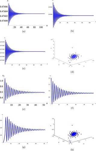
In this section, we will present simulation to verify not only obtained results but also exhibits that (7(7) $\begin{array}{rl}{x}_{n+1}& =\frac{{\alpha }_1{\mathrm{e}}^{-x_n}+{\alpha }_2{\mathrm{e}}^{-x_{n-1}}}{{\alpha }_3+{\alpha }_1{y}_n+{\alpha }_2{y}_{n-1}},\\ y_{n+1}& =\frac{{\alpha }_4{\mathrm{e}}^{-y_n}+{\alpha }_5{\mathrm{e}}^{-y_{n-1}}}{{\alpha }_6+{\alpha }_4{z}_n+{\alpha }_5{z}_{n-1}},\\ z_{n+1}& =\frac{{\alpha }_7{\mathrm{e}}^{-z_n}+{\alpha }_8{\mathrm{e}}^{-z_{n-1}}}{{\alpha }_9+{\alpha }_7{x}_n+{\alpha }_8{x}_{n-1}},\end{array}$(7) ) undergoes a supercritical hopf bifurcation. For instance, if ${\alpha }_i(i=1,\dots ,9)$ are 13, 0.24, 8, 12, 0.1, 5, 5,0.14, 4, then condition (22(22) $\begin{array}{rl}& \frac{\left({\alpha }_1+{\alpha }_2\right){\mathrm{e}}^{-L_1}}{{\alpha }_3+\left({\alpha }_1+{\alpha }_2\right)L_2}+\frac{\left({\alpha }_7+{\alpha }_8\right){\mathrm{e}}^{-L_3}}{{\alpha }_9+\left({\alpha }_7+{\alpha }_8\right)L_1}\\ & +\frac{\left({\alpha }_4+{\alpha }_5\right){\mathrm{e}}^{-L_2}}{{\alpha }_6+\left({\alpha }_4+{\alpha }_5\right)L_3}\\ & +\frac{\left({\alpha }_1{\alpha }_4+{\alpha }_1{\alpha }_5\right){\mathrm{e}}^{-L_1-L_2}}{({\alpha }_6+({\alpha }_4+{\alpha }_5\left)L_3\right)({\alpha }_3+({\alpha }_1+{\alpha }_2\left)L_2\right)}\\ & +\frac{\left({\alpha }_4{\alpha }_7+{\alpha }_5{\alpha }_7+{\alpha }_4{\alpha }_8\right){\mathrm{e}}^{-L_2-L_3}}{({\alpha }_6+({\alpha }_4+{\alpha }_5\left)L_3\right)({\alpha }_9+({\alpha }_7+{\alpha }_8\left)L_1\right)}\\ & +\frac{{\alpha }_1{\alpha }_7{\mathrm{e}}^{-L_1-L_3}}{({\alpha }_9+({\alpha }_7+{\alpha }_8\left)L_1\right)({\alpha }_3+({\alpha }_1+{\alpha }_2\left)L_2\right)}\\ & +\frac{{\alpha }_1{\alpha }_8{\mathrm{e}}^{-L_1-L_2}}{({\alpha }_9+({\alpha }_7+{\alpha }_8\left)L_1\right)({\alpha }_3+({\alpha }_1+{\alpha }_2\left)L_2\right)}\\ & +\frac{\begin{array}{c}\left({\alpha }_2{\alpha }_5{\alpha }_8+{\alpha }_1{\alpha }_4{\alpha }_7+{\alpha }_1{\alpha }_5{\alpha }_8\right.\\ +\left.{\alpha }_2{\alpha }_5{\alpha }_7+{\alpha }_2{\alpha }_4{\alpha }_8\right){\mathrm{e}}^{-L_1-L_2-L_3}\end{array}}{\begin{array}{c}({\alpha }_9+({\alpha }_7+{\alpha }_8\left)L_1\right)({\alpha }_3+({\alpha }_1\\ +{\alpha }_2\left)L_2\right)({\alpha }_6+({\alpha }_4+{\alpha }_5\left)L_3\right)\end{array}}\\ & +\frac{\begin{array}{c}\left({\alpha }_2{\alpha }_5{\alpha }_8+{\alpha }_1{\alpha }_5{\alpha }_8\right.\\ +\left.{\alpha }_2{\alpha }_5{\alpha }_7+{\alpha }_5{\alpha }_1{\alpha }_7\right)U_1{U}_2{U}_3\end{array}}{\begin{array}{c}({\alpha }_9+({\alpha }_7+{\alpha }_8\left)L_1\right)({\alpha }_3+({\alpha }_1\\ +{\alpha }_2\left)L_2\right)({\alpha }_6+({\alpha }_4+{\alpha }_5\left)L_3\right)\end{array}}<1;\end{array}$(22) ) holds, i.e. $\begin{array}{rl}& \frac{({\alpha }_1+{\alpha }_2){\mathrm{e}}^{-L_1}}{{\alpha }_3+({\alpha }_1+{\alpha }_2)L_2}+\frac{({\alpha }_7+{\alpha }_8){\mathrm{e}}^{-L_3}}{{\alpha }_9+({\alpha }_7+{\alpha }_8)L_1}\\ & +\frac{({\alpha }_1{\alpha }_4+{\alpha }_1{\alpha }_5){\mathrm{e}}^{-L_1-L_2}}{({\alpha }_6+({\alpha }_4+{\alpha }_5\left)L_3\right)({\alpha }_3+({\alpha }_1+{\alpha }_2\left)L_2\right)}\\ & +\frac{({\alpha }_4+{\alpha }_5){\mathrm{e}}^{-L_2}}{{\alpha }_6+({\alpha }_4+{\alpha }_5)L_3}\\ & +\frac{({\alpha }_4{\alpha }_7+{\alpha }_5{\alpha }_7+{\alpha }_4{\alpha }_8){\mathrm{e}}^{-L_2-L_3}}{({\alpha }_6+({\alpha }_4+{\alpha }_5\left)L_3\right)({\alpha }_9+({\alpha }_7+{\alpha }_8\left)L_1\right)}\\ & +\frac{{\alpha }_1{\alpha }_7{\mathrm{e}}^{-L_1-L_3}}{({\alpha }_9+({\alpha }_7+{\alpha }_8\left)L_1\right)({\alpha }_3+({\alpha }_1+{\alpha }_2\left)L_2\right)}\\ & +\frac{{\alpha }_1{\alpha }_8{\mathrm{e}}^{-L_1-L_2}}{({\alpha }_9+({\alpha }_7+{\alpha }_8\left)L_1\right)({\alpha }_3+({\alpha }_1+{\alpha }_2\left)L_2\right)}\\ & +\frac{\begin{array}{c}({\alpha }_2{\alpha }_5{\alpha }_8+{\alpha }_1{\alpha }_4{\alpha }_7+{\alpha }_1{\alpha }_5{\alpha }_8\\ +{\alpha }_2{\alpha }_5{\alpha }_7+{\alpha }_2{\alpha }_4{\alpha }_8){\mathrm{e}}^{-L_1-L_2-L_3}\end{array}}{\begin{array}{c}({\alpha }_9+({\alpha }_7+{\alpha }_8\left)L_1\right)({\alpha }_3+({\alpha }_1\\ +{\alpha }_2\left)L_2\right)({\alpha }_6+({\alpha }_4+{\alpha }_5\left)L_3\right)\end{array}}\\ & +\frac{\begin{array}{c}({\alpha }_2{\alpha }_5{\alpha }_8+{\alpha }_1{\alpha }_5{\alpha }_8+{\alpha }_2{\alpha }_5{\alpha }_7\\ +{\alpha }_5{\alpha }_1{\alpha }_7)U_1{U}_2{U}_3\end{array}}{\begin{array}{c}({\alpha }_9+({\alpha }_7+{\alpha }_8\left)L_1\right)({\alpha }_3\\ +({\alpha }_1+{\alpha }_2)L_2\left)\right({\alpha }_6+({\alpha }_4+{\alpha }_5)L_3)\end{array}}\\ & =0.06223205265987121987645<1,\end{array}$ 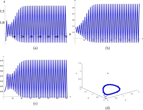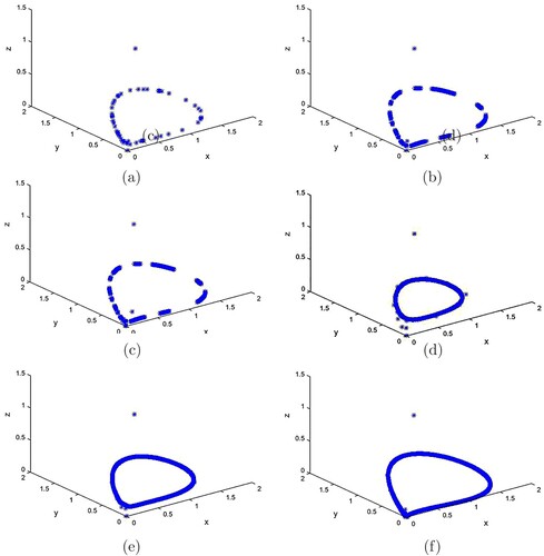which clearly indicate the fact that the unique positive equilibrium point $(0.4760299878571522,0.9249913676665756,0.4718569265705974)$ of (7(7) $\begin{array}{rl}{x}_{n+1}& =\frac{{\alpha }_1{\mathrm{e}}^{-x_n}+{\alpha }_2{\mathrm{e}}^{-x_{n-1}}}{{\alpha }_3+{\alpha }_1{y}_n+{\alpha }_2{y}_{n-1}},\\ y_{n+1}& =\frac{{\alpha }_4{\mathrm{e}}^{-y_n}+{\alpha }_5{\mathrm{e}}^{-y_{n-1}}}{{\alpha }_6+{\alpha }_4{z}_n+{\alpha }_5{z}_{n-1}},\\ z_{n+1}& =\frac{{\alpha }_7{\mathrm{e}}^{-z_n}+{\alpha }_8{\mathrm{e}}^{-z_{n-1}}}{{\alpha }_9+{\alpha }_7{x}_n+{\alpha }_8{x}_{n-1}},\end{array}$(7) ) is locally stable (see Figure 1(a–c)). Moreover, for said values, condition (33(33) $\begin{array}{rl}& \left({\alpha }_1+{\alpha }_2\right){\mathrm{e}}^{-L_1}<\left(2\overline{x}-U_1\right)\left({\alpha }_3+\left({\alpha }_1+{\alpha }_2\right)L_2\right),\\ & \left({\alpha }_4+{\alpha }_5\right){\mathrm{e}}^{-L_2}<\left(2\overline{y}-U_2\right)\left({\alpha }_6+\left({\alpha }_4+{\alpha }_5\right)L_3\right),\\ & \left({\alpha }_7+{\alpha }_8\right){\mathrm{e}}^{-L_3}<\left(2\overline{z}-U_3\right)\left({\alpha }_9+\left({\alpha }_7+{\alpha }_8\right)L_1\right).\end{array}$(33) ) also hold, i.e. $({\alpha }_1+{\alpha }_2){\mathrm{e}}^{-L_1}=6.681696991393797<(2\overline{x}-U_1)({\alpha }_3+({\alpha }_1+{\alpha }_2\left)L_2\right)=12.429286853034514,({\alpha }_4+{\alpha }_5){\mathrm{e}}^{-L_2}=3.6342836498120694<\left(2\overline{y}-U_2\right)({\alpha }_6+({\alpha }_4+{\alpha }_5\left)L_3\right)=10.799584645301376,({\alpha }_7+{\alpha }_8){\mathrm{e}}^{-L_3}=4.587592155111493<(2\overline{z}-U_3)\left({\alpha }_9+\right({\alpha }_7+{\alpha }_8\left)L_1\right)=9.412421234484496$, which indicates that positive equilibrium point is globally stable (see Figure 1(d)), and hence, these computations agree with theoretical results. Similarly, for choosing parameters ${\alpha }_i(i=1,\dots ,9)$ as $18,0.24,8,12,0.1,5,5,0.4,4$, then from Figure 1(e–g), the unique +ve equilibrium point $(0.5869973072136292,0.9252376829323564,0.4861615443150309)$ of (7(7) $\begin{array}{rl}{x}_{n+1}& =\frac{{\alpha }_1{\mathrm{e}}^{-x_n}+{\alpha }_2{\mathrm{e}}^{-x_{n-1}}}{{\alpha }_3+{\alpha }_1{y}_n+{\alpha }_2{y}_{n-1}},\\ y_{n+1}& =\frac{{\alpha }_4{\mathrm{e}}^{-y_n}+{\alpha }_5{\mathrm{e}}^{-y_{n-1}}}{{\alpha }_6+{\alpha }_4{z}_n+{\alpha }_5{z}_{n-1}},\\ z_{n+1}& =\frac{{\alpha }_7{\mathrm{e}}^{-z_n}+{\alpha }_8{\mathrm{e}}^{-z_{n-1}}}{{\alpha }_9+{\alpha }_7{x}_n+{\alpha }_8{x}_{n-1}},\end{array}$(7) ) is stable and its corresponding attractor is shown in Figure 1(h). But if ${\alpha }_i(i=1,\dots ,9)$ are 18, 0.24, 8, 20, 0.1, 5, 5,0.4, 4, then from Figure 2(a–c), the unique positive equilibrium point $(0.12206059150567157,3.3039362385056905,0.33608644648845903)$ of (7(7) $\begin{array}{rl}{x}_{n+1}& =\frac{{\alpha }_1{\mathrm{e}}^{-x_n}+{\alpha }_2{\mathrm{e}}^{-x_{n-1}}}{{\alpha }_3+{\alpha }_1{y}_n+{\alpha }_2{y}_{n-1}},\\ y_{n+1}& =\frac{{\alpha }_4{\mathrm{e}}^{-y_n}+{\alpha }_5{\mathrm{e}}^{-y_{n-1}}}{{\alpha }_6+{\alpha }_4{z}_n+{\alpha }_5{z}_{n-1}},\\ z_{n+1}& =\frac{{\alpha }_7{\mathrm{e}}^{-z_n}+{\alpha }_8{\mathrm{e}}^{-z_{n-1}}}{{\alpha }_9+{\alpha }_7{x}_n+{\alpha }_8{x}_{n-1}},\end{array}$(7) ) is unstable and in the meantime stable closed curve appeared which is depicted in Figure 2(d). The appearance of the stable closed curve implies that (7(7) $\begin{array}{rl}{x}_{n+1}& =\frac{{\alpha }_1{\mathrm{e}}^{-x_n}+{\alpha }_2{\mathrm{e}}^{-x_{n-1}}}{{\alpha }_3+{\alpha }_1{y}_n+{\alpha }_2{y}_{n-1}},\\ y_{n+1}& =\frac{{\alpha }_4{\mathrm{e}}^{-y_n}+{\alpha }_5{\mathrm{e}}^{-y_{n-1}}}{{\alpha }_6+{\alpha }_4{z}_n+{\alpha }_5{z}_{n-1}},\\ z_{n+1}& =\frac{{\alpha }_7{\mathrm{e}}^{-z_n}+{\alpha }_8{\mathrm{e}}^{-z_{n-1}}}{{\alpha }_9+{\alpha }_7{x}_n+{\alpha }_8{x}_{n-1}},\end{array}$(7) ) undergoes a supercritical hopf bifurcation. More bifurcation diagrams subject to $x_{-1}=0.07,x_0=0.2,y_{-1}=1.9,y_0=1.4,z_{-1}=0.9$ and $z_0=0.4$ are plotted in Figure 3.

Figure 1. Trajectories for (7(7) $\begin{array}{rl}{x}_{n+1}& =\frac{{\alpha }_1{\mathrm{e}}^{-x_n}+{\alpha }_2{\mathrm{e}}^{-x_{n-1}}}{{\alpha }_3+{\alpha }_1{y}_n+{\alpha }_2{y}_{n-1}},\\ y_{n+1}& =\frac{{\alpha }_4{\mathrm{e}}^{-y_n}+{\alpha }_5{\mathrm{e}}^{-y_{n-1}}}{{\alpha }_6+{\alpha }_4{z}_n+{\alpha }_5{z}_{n-1}},\\ z_{n+1}& =\frac{{\alpha }_7{\mathrm{e}}^{-z_n}+{\alpha }_8{\mathrm{e}}^{-z_{n-1}}}{{\alpha }_9+{\alpha }_7{x}_n+{\alpha }_8{x}_{n-1}},\end{array}$(7) ) with $x_s,y_s,z_s(s=-1,0)$ are 1.7, 0.2, 0.9, 1.4, 0.9, 0.24.

Figure 2. Trajectories for (7(7) $\begin{array}{rl}{x}_{n+1}& =\frac{{\alpha }_1{\mathrm{e}}^{-x_n}+{\alpha }_2{\mathrm{e}}^{-x_{n-1}}}{{\alpha }_3+{\alpha }_1{y}_n+{\alpha }_2{y}_{n-1}},\\ y_{n+1}& =\frac{{\alpha }_4{\mathrm{e}}^{-y_n}+{\alpha }_5{\mathrm{e}}^{-y_{n-1}}}{{\alpha }_6+{\alpha }_4{z}_n+{\alpha }_5{z}_{n-1}},\\ z_{n+1}& =\frac{{\alpha }_7{\mathrm{e}}^{-z_n}+{\alpha }_8{\mathrm{e}}^{-z_{n-1}}}{{\alpha }_9+{\alpha }_7{x}_n+{\alpha }_8{x}_{n-1}},\end{array}$(7) ) with $x_s,y_s,z_s(s=-1,0)$ are 0.07, 0.2, 1.9, 1.4, 0.9, 0.4.

Figure 3. Supercritical N–S bifurcation for (7(7) $\begin{array}{rl}{x}_{n+1}& =\frac{{\alpha }_1{\mathrm{e}}^{-x_n}+{\alpha }_2{\mathrm{e}}^{-x_{n-1}}}{{\alpha }_3+{\alpha }_1{y}_n+{\alpha }_2{y}_{n-1}},\\ y_{n+1}& =\frac{{\alpha }_4{\mathrm{e}}^{-y_n}+{\alpha }_5{\mathrm{e}}^{-y_{n-1}}}{{\alpha }_6+{\alpha }_4{z}_n+{\alpha }_5{z}_{n-1}},\\ z_{n+1}& =\frac{{\alpha }_7{\mathrm{e}}^{-z_n}+{\alpha }_8{\mathrm{e}}^{-z_{n-1}}}{{\alpha }_9+{\alpha }_7{x}_n+{\alpha }_8{x}_{n-1}},\end{array}$(7) ): (a) ${\alpha }_s(s=1,\dots ,6)$ are 18, 0.24, 13, 20, 0.1, 5, 5,0.4, 4, (b) 18, 0.24, 13, 20.5, 0.1, 5, 5,0.4, 4, (c) 18, 0.24, 13, 20.57, 0.1, 5, 5,0.4, 4, (d) 18, 0.24, 13, 21.5, 0.1, 5, 5,0.4, 4, (e) 18, 0.24, 13, 22.5, 0.1, 5, 5,0.4, 4 and (f) 18, 0.24, 13, 23.125, 0.1, 5, 5,0.4, 4.

9. Conclusion

The presented work is about the dynamical properties of the three-directional system of difference equations, that is the extension of the work studied by Bozkurt [5] and Khan and Qureshi [6]. We have proved that the +ve solution $\{{\mathrm{\Omega }}_n{\}}_{n=-1}^{\mathrm{\infty }}$ of (7(7) $\begin{array}{rl}{x}_{n+1}& =\frac{{\alpha }_1{\mathrm{e}}^{-x_n}+{\alpha }_2{\mathrm{e}}^{-x_{n-1}}}{{\alpha }_3+{\alpha }_1{y}_n+{\alpha }_2{y}_{n-1}},\\ y_{n+1}& =\frac{{\alpha }_4{\mathrm{e}}^{-y_n}+{\alpha }_5{\mathrm{e}}^{-y_{n-1}}}{{\alpha }_6+{\alpha }_4{z}_n+{\alpha }_5{z}_{n-1}},\\ z_{n+1}& =\frac{{\alpha }_7{\mathrm{e}}^{-z_n}+{\alpha }_8{\mathrm{e}}^{-z_{n-1}}}{{\alpha }_9+{\alpha }_7{x}_n+{\alpha }_8{x}_{n-1}},\end{array}$(7) ) is bounded and persists, i.e. $L_1\le {\displaystyle \underset{n\to \mathrm{\infty }}{lim}inf{x}_n\le \underset{n\to \mathrm{\infty }}{lim}sup{x}_n\le U_1}$, $L_2\le {\displaystyle \underset{n\to \mathrm{\infty }}{lim}inf{y}_n\le \underset{n\to \mathrm{\infty }}{lim}sup{y}_n\le U_2}$, $L_3\le {\displaystyle \underset{n\to \mathrm{\infty }}{lim}inf{z}_n\le \underset{n\to \mathrm{\infty }}{lim}sup{z}_n\le U_3}$, and the set $[L_1,U_1]\times [L_2,U_2]\times [L_3,U_3]$ where $\begin{array}{rl}{L}_1& =\frac{({\alpha }_1+{\alpha }_2){\mathrm{e}}^{-\left(\right({\alpha }_1+{\alpha }_2\left)/{\alpha }_3\right)}}{{\alpha }_3+({\alpha }_1+{\alpha }_2)\left(\right({\alpha }_4+{\alpha }_5\left)/{\alpha }_6\right)},U_1=\frac{{\alpha }_1+{\alpha }_2}{{\alpha }_3},\\ L_2& =\frac{({\alpha }_4+{\alpha }_5){\mathrm{e}}^{-\left(\right({\alpha }_4+{\alpha }_5\left)/{\alpha }_6\right)}}{{\alpha }_6+({\alpha }_4+{\alpha }_5)\left(\right({\alpha }_7+{\alpha }_8\left)/{\alpha }_9\right)},\\ U_2& =\frac{{\alpha }_4+{\alpha }_5}{{\alpha }_6},\\ L_3& =\frac{({\alpha }_7+{\alpha }_8){\mathrm{e}}^{-\left(\right({\alpha }_7+{\alpha }_8\left)/{\alpha }_9\right)}}{{\alpha }_9+({\alpha }_7+{\alpha }_8)\left(\right({\alpha }_1+{\alpha }_2\left)/{\alpha }_3\right)},U_3=\frac{{\alpha }_7+{\alpha }_8}{{\alpha }_9}\end{array}$ is invariant rectangle. Furthermore, we have proved that (7(7) $\begin{array}{rl}{x}_{n+1}& =\frac{{\alpha }_1{\mathrm{e}}^{-x_n}+{\alpha }_2{\mathrm{e}}^{-x_{n-1}}}{{\alpha }_3+{\alpha }_1{y}_n+{\alpha }_2{y}_{n-1}},\\ y_{n+1}& =\frac{{\alpha }_4{\mathrm{e}}^{-y_n}+{\alpha }_5{\mathrm{e}}^{-y_{n-1}}}{{\alpha }_6+{\alpha }_4{z}_n+{\alpha }_5{z}_{n-1}},\\ z_{n+1}& =\frac{{\alpha }_7{\mathrm{e}}^{-z_n}+{\alpha }_8{\mathrm{e}}^{-z_{n-1}}}{{\alpha }_9+{\alpha }_7{x}_n+{\alpha }_8{x}_{n-1}},\end{array}$(7) ) has a unique +ve equilibrium point: Υ if $\begin{array}{rl}& \frac{\begin{array}{c}{\mathrm{e}}^{-\left(\right({\mathrm{e}}^{-U_3}/L_3)-({\alpha }_9/({\alpha }_7+{\alpha }_8)\left)\right)}(U_3+1){\mathrm{e}}^{-L_3}\left(\right({\alpha }_9/({\alpha }_7+{\alpha }_8))-\\ \left({\mathrm{e}}^{-U_3}/L_3\right)-1)\end{array}}{U_3^2\left(\right({\mathrm{e}}^{-L_3}/L_3)-({\alpha }_9/({\alpha }_7+{\alpha }_8)){)}^2}\\ & \times {\mathrm{e}}^{-\left(\frac{{\mathrm{e}}^{-\left(\right({\mathrm{e}}^{-L_3}/U_3)-({\alpha }_9/({\alpha }_7+{\alpha }_8)\left)\right)}}{\left({\mathrm{e}}^{-L_3}/L_3\right)-\left({\alpha }_9/\right({\alpha }_7+{\alpha }_8\left)\right)}-\frac{{\alpha }_3}{{\alpha }_1+{\alpha }_2}\right)}(\mathrm{\Lambda }+1)<{\mathrm{\Lambda }}^2,\end{array}$ where Λ is defined in (21(21) $\begin{array}{r}\mathrm{\Lambda }=\frac{{\mathrm{e}}^{-\left(\left({\mathrm{e}}^{-U_3}/L_3\right)-\left({\alpha }_9/\right({\alpha }_7+{\alpha }_8\left)\right)\right)}}{\left({\mathrm{e}}^{-L_3}/L_3\right)-\left({\alpha }_9/\right({\alpha }_7+{\alpha }_8\left)\right)}-\frac{{\alpha }_3}{{\alpha }_1+{\alpha }_2}.\end{array}$(21) ). By linear stability, we have explored the local dynamics about Υ and proved that it is sink (respectively unstable) if (22(22) $\begin{array}{rl}& \frac{\left({\alpha }_1+{\alpha }_2\right){\mathrm{e}}^{-L_1}}{{\alpha }_3+\left({\alpha }_1+{\alpha }_2\right)L_2}+\frac{\left({\alpha }_7+{\alpha }_8\right){\mathrm{e}}^{-L_3}}{{\alpha }_9+\left({\alpha }_7+{\alpha }_8\right)L_1}\\ & +\frac{\left({\alpha }_4+{\alpha }_5\right){\mathrm{e}}^{-L_2}}{{\alpha }_6+\left({\alpha }_4+{\alpha }_5\right)L_3}\\ & +\frac{\left({\alpha }_1{\alpha }_4+{\alpha }_1{\alpha }_5\right){\mathrm{e}}^{-L_1-L_2}}{({\alpha }_6+({\alpha }_4+{\alpha }_5\left)L_3\right)({\alpha }_3+({\alpha }_1+{\alpha }_2\left)L_2\right)}\\ & +\frac{\left({\alpha }_4{\alpha }_7+{\alpha }_5{\alpha }_7+{\alpha }_4{\alpha }_8\right){\mathrm{e}}^{-L_2-L_3}}{({\alpha }_6+({\alpha }_4+{\alpha }_5\left)L_3\right)({\alpha }_9+({\alpha }_7+{\alpha }_8\left)L_1\right)}\\ & +\frac{{\alpha }_1{\alpha }_7{\mathrm{e}}^{-L_1-L_3}}{({\alpha }_9+({\alpha }_7+{\alpha }_8\left)L_1\right)({\alpha }_3+({\alpha }_1+{\alpha }_2\left)L_2\right)}\\ & +\frac{{\alpha }_1{\alpha }_8{\mathrm{e}}^{-L_1-L_2}}{({\alpha }_9+({\alpha }_7+{\alpha }_8\left)L_1\right)({\alpha }_3+({\alpha }_1+{\alpha }_2\left)L_2\right)}\\ & +\frac{\begin{array}{c}\left({\alpha }_2{\alpha }_5{\alpha }_8+{\alpha }_1{\alpha }_4{\alpha }_7+{\alpha }_1{\alpha }_5{\alpha }_8\right.\\ +\left.{\alpha }_2{\alpha }_5{\alpha }_7+{\alpha }_2{\alpha }_4{\alpha }_8\right){\mathrm{e}}^{-L_1-L_2-L_3}\end{array}}{\begin{array}{c}({\alpha }_9+({\alpha }_7+{\alpha }_8\left)L_1\right)({\alpha }_3+({\alpha }_1\\ +{\alpha }_2\left)L_2\right)({\alpha }_6+({\alpha }_4+{\alpha }_5\left)L_3\right)\end{array}}\\ & +\frac{\begin{array}{c}\left({\alpha }_2{\alpha }_5{\alpha }_8+{\alpha }_1{\alpha }_5{\alpha }_8\right.\\ +\left.{\alpha }_2{\alpha }_5{\alpha }_7+{\alpha }_5{\alpha }_1{\alpha }_7\right)U_1{U}_2{U}_3\end{array}}{\begin{array}{c}({\alpha }_9+({\alpha }_7+{\alpha }_8\left)L_1\right)({\alpha }_3+({\alpha }_1\\ +{\alpha }_2\left)L_2\right)({\alpha }_6+({\alpha }_4+{\alpha }_5\left)L_3\right)\end{array}}<1;\end{array}$(22) ) (respectively (23(23) $\begin{array}{rl}& \frac{\left({\alpha }_1+{\alpha }_2\right){\mathrm{e}}^{-U_1}}{{\alpha }_3+\left({\alpha }_1+{\alpha }_2\right)U_2}+\frac{\left({\alpha }_7+{\alpha }_8\right){\mathrm{e}}^{-U_3}}{{\alpha }_9+\left({\alpha }_7+{\alpha }_8\right)U_1}\\ & +\frac{\left({\alpha }_4+{\alpha }_5\right){\mathrm{e}}^{-U_2}}{{\alpha }_6+\left({\alpha }_4+{\alpha }_5\right)U_3}\\ & +\frac{\left({\alpha }_1{\alpha }_4+{\alpha }_1{\alpha }_5\right){\mathrm{e}}^{-U_1-U_2}}{({\alpha }_6+({\alpha }_4+{\alpha }_5\left)U_3\right)({\alpha }_3+({\alpha }_1+{\alpha }_2\left)U_2\right)}\\ & +\frac{\left({\alpha }_4{\alpha }_7+{\alpha }_5{\alpha }_7+{\alpha }_4{\alpha }_8\right){\mathrm{e}}^{-U_2-U_3}}{({\alpha }_6+({\alpha }_4+{\alpha }_5\left)U_3\right)({\alpha }_9+({\alpha }_7+{\alpha }_8\left)U_1\right)}\\ & +\frac{{\alpha }_1{\alpha }_7{\mathrm{e}}^{-U_1-U_3}}{({\alpha }_9+({\alpha }_7+{\alpha }_8\left)U_1\right)({\alpha }_3+({\alpha }_1+{\alpha }_2\left)U_2\right)}\\ & +\frac{{\alpha }_1{\alpha }_8{\mathrm{e}}^{-U_1-U_2}}{({\alpha }_9+({\alpha }_7+{\alpha }_8\left)U_1\right)({\alpha }_3+({\alpha }_1+{\alpha }_2\left)U_2\right)}\\ & +\frac{\begin{array}{c}\left({\alpha }_2{\alpha }_5{\alpha }_8+{\alpha }_1{\alpha }_4{\alpha }_7+{\alpha }_1{\alpha }_5{\alpha }_8\right.\\ +\left.{\alpha }_2{\alpha }_5{\alpha }_7+{\alpha }_2{\alpha }_4{\alpha }_8\right){\mathrm{e}}^{-U_1-U_2-U_3}\end{array}}{\begin{array}{c}({\alpha }_9+({\alpha }_7+{\alpha }_8\left)U_1\right)({\alpha }_3+({\alpha }_1\\ +{\alpha }_2\left)U_2\right)({\alpha }_6+({\alpha }_4+{\alpha }_5\left)U_3\right)\end{array}}\\ & +\frac{\begin{array}{c}\left({\alpha }_2{\alpha }_5{\alpha }_8+{\alpha }_1{\alpha }_5{\alpha }_8+{\alpha }_2{\alpha }_5{\alpha }_7\right.\\ +\left.{\alpha }_5{\alpha }_1{\alpha }_7\right)L_1{L}_2{L}_3\end{array}}{\begin{array}{c}({\alpha }_9+({\alpha }_7+{\alpha }_8\left)U_1\right)({\alpha }_3+({\alpha }_1\\ +{\alpha }_2\left)U_2\right)({\alpha }_6+({\alpha }_4+{\alpha }_5\left)U_3\right)\end{array}}>1.\end{array}$(23) )) holds. By constructing the discrete-time discrete-time Lyapunov function, we explored that Υ of (7(7) $\begin{array}{rl}{x}_{n+1}& =\frac{{\alpha }_1{\mathrm{e}}^{-x_n}+{\alpha }_2{\mathrm{e}}^{-x_{n-1}}}{{\alpha }_3+{\alpha }_1{y}_n+{\alpha }_2{y}_{n-1}},\\ y_{n+1}& =\frac{{\alpha }_4{\mathrm{e}}^{-y_n}+{\alpha }_5{\mathrm{e}}^{-y_{n-1}}}{{\alpha }_6+{\alpha }_4{z}_n+{\alpha }_5{z}_{n-1}},\\ z_{n+1}& =\frac{{\alpha }_7{\mathrm{e}}^{-z_n}+{\alpha }_8{\mathrm{e}}^{-z_{n-1}}}{{\alpha }_9+{\alpha }_7{x}_n+{\alpha }_8{x}_{n-1}},\end{array}$(7) ) is globally asymptotically stable if $({\alpha }_1+{\alpha }_2){\mathrm{e}}^{-L_1}<(2\overline{x}-U_1)({\alpha }_3+({\alpha }_1+{\alpha }_2\left)L_2\right)$, $({\alpha }_4+{\alpha }_5){\mathrm{e}}^{-L_2}<\left(2\overline{y}-U_2\right)\left({\alpha }_6+\right({\alpha }_4+{\alpha }_5\left)L_3\right)$ and $({\alpha }_7+{\alpha }_8){\mathrm{e}}^{-L_3}<(2\overline{z}-U_3)\left({\alpha }_9+\right({\alpha }_7+{\alpha }_8\left)L_1\right)$ hold. We have also explored the rate of convergence that converges to unique +ve equilibrium Υ. Finally, simulations are presented to verify obtained results. These simulations not only verify our obtained results but also proved that (7(7) $\begin{array}{rl}{x}_{n+1}& =\frac{{\alpha }_1{\mathrm{e}}^{-x_n}+{\alpha }_2{\mathrm{e}}^{-x_{n-1}}}{{\alpha }_3+{\alpha }_1{y}_n+{\alpha }_2{y}_{n-1}},\\ y_{n+1}& =\frac{{\alpha }_4{\mathrm{e}}^{-y_n}+{\alpha }_5{\mathrm{e}}^{-y_{n-1}}}{{\alpha }_6+{\alpha }_4{z}_n+{\alpha }_5{z}_{n-1}},\\ z_{n+1}& =\frac{{\alpha }_7{\mathrm{e}}^{-z_n}+{\alpha }_8{\mathrm{e}}^{-z_{n-1}}}{{\alpha }_9+{\alpha }_7{x}_n+{\alpha }_8{x}_{n-1}},\end{array}$(7) ) undergoes a supercritical hopf bifurcation.

Acknowledgments

This work was supported by the Higher Education Commission of Pakistan.

Disclosure statement

No potential conflict of interest was reported by the authors.

Additional information

Funding

.

References

El-Metwally E, Grove EA, Ladas G, et al. On the difference equation xn+1=α1+α2xn−1e−xn. Nonlinear Anal. 2001;47:4623–4634. doi: 10.1016/S0362-546X(01)00575-2
Papaschinopoulos G, Radin M, Schinas CJ. Study of the asymptotic behavior of the solutions of three systems of difference equations of exponential form. Appl Math Comput. 2012;218:5310–5318.
Garić-Demirović M, Kulenović MRS. Dynamics of an anti-competitive two dimensional rational system of difference equations. Sarajevo J Math. 2014;7(19):39–56.
?Mathematical formulae have been encoded as MathML and are displayed in this HTML version using MathJax in order to improve their display. Uncheck the box to turn MathJax off. This feature requires Javascript. Click on a formula to zoom.
(22)
Assuming that (Equation22