Disturbance solutions for the long–short-wave interaction system using bi-random Riccati–Bernoulli sub-ODE method

Abstract

This article applied the Riccati–Bernoulli (RB) sub-ODE method in order to get new exact solutions for the long–short-wave interaction (LS) equations. Namely, we obtain deterministic and random solutions, since we consider the proposed method in deterministic and random cases. The RB sub-ODE technique gives the travelling wave solutions in forms of hyperbolic, trigonometric and rational functions. It is shown that the proposed method gives a robust mathematical tool for solving nonlinear wave equations in applied science. Furthermore, some bi-random variables and some random distributions are used in random case corresponding to the LS system. The stability for the obtained solutions in random case is considered. In addition, there is a display of several numerical simulations, which helps to understand the physical phenomena of these soliton wave solutions.

Keywords:

• Riccati–Bernoulli sub-ODE technique
• long–short-wave interaction equations
• Bäcklund transformation
• travelling wave solutions
• exact solutions
• random distributions
• second-order random variables
• stability

Mathematics Subject Classification (2010):

• 35A99
• 83C15
• 62P99
• 65Z05
• 74J35

1. Introduction

In recent years, many researchers have tried to find exact solutions of the nonlinear partial differential equations (NPDEs), which play an important role in nonlinear science and engineering, for instance, fluid mechanics, meteorology, plasma physics, solid state physics, heat flow and chemical engineering [1–14]. As a result, many new methods have been successfully investigated and proposed like tanh–sech method [15], homogeneous balance method [16], exp-function method [17], Riccati–Bernoulli (RB) sub-ODE method [18–20], sine-cosine method [21], He's variational method [22], homotopy perturbation method [23], trigonometric function series method [24], $\left(G^{\mathrm{\prime }}/G\right)-$expansion method [25], Jacobi elliptic function method [26] and trial solution method [27]. Furthermore, there are further interesting analytical and numerical techniques for obtaining solutions of NPDEs, see [28–32].

Since Riccati differential equations are related to various serious problems of applied science, finding their solutions is a task of great importance, [33–37]. Recently, one of the important method that consider such equations is the RB sub-ODE approach. In this article, the RB sub-ODE scheme is used in investigating the solutions for the long–short-wave interaction (LS) system. This system depicts the interaction between one long longitudinal wave and one short transverse wave propagating in a generalized elastic medium [38]. As a consequence, this technique provides new infinite solutions of NPDEs utilizing a Bäcklund transformation. Moreover, we introduce a new combination between two vital branches of science, namely partial differential equations and applied statistics. In this work we show that how this approach is so interesting and can be generalized to many models of NPDEs.

In this work, we study our new technique in a random case since the wave transportation containing bi-random variables and some random distributions are used. Many papers discussed the random models such as stochastic partial differential Equations [39–41] but in this study we develop the deterministic case for this method to be in random case. Indeed, we introduce the stability and convergence analysis to give their conditions for our method. To the best of our knowledge, no antecedent articles have been achieved utilizing RB sub-ODE method for solving the LS system in deterministic and stochastic cases.

There is no doubt that discussing the real-life applications with some disturbances such as the parameters be random variables is acceptable than in the deterministic case. In this paper, some random distributions are used in order to clarify that the effect of random variables is so interesting. Additionally, using the random distributions open up a wide range of physical meaning for the solutions. Of course, the randomness with in the solutions will be appear on the qualitative study such as stability, convergence, etc. So, we investigate this effect in some distributions such as beta distribution, Poisson distribution, etc.

2. Description of the method

We introduce RB sub-ODE technique to construct the solutions for NPDEs. The main steps of this method are [18]:

Step 1. Consider an NPDE as (1) $\mathrm{\Phi }(\chi ,{\chi }_t,{\chi }_x,{\chi }_{tt},{\chi }_{xx},\dots .)=0.$(1) Utilizing the wave transformation (2) $\chi (x,t)=\chi \left(\eta \right),\eta =kx+vt,$(2) converts Equation (2(2) $\chi (x,t)=\chi \left(\eta \right),\eta =kx+vt,$(2) ) to an ODE (3) $\mathrm{\Psi }(\chi ,{\chi }^{\prime },{\chi }^{″},{\chi }^{‴},\dots ..)=0.$(3)

Step 2. Suppose that the solution $u\left(\eta \right)$ of Equation (3(3) $\mathrm{\Psi }(\chi ,{\chi }^{\prime },{\chi }^{″},{\chi }^{‴},\dots ..)=0.$(3) ) obeys (4) ${\chi }^{\prime }=a{\chi }^{2-r}+b\chi +c{\chi }^r,$(4) in which the constants a, b, c and r are determined later. Using Equation (4(4) ${\chi }^{\prime }=a{\chi }^{2-r}+b\chi +c{\chi }^r,$(4) ), gives (5) $\begin{array}{rl}{\chi }^{″}& =ab(3-r){\chi }^{2-r}+a^2(2-r){\chi }^{3-2r}+r{c}^2{\chi }^{2r-1}\\ & +bc(r+1){\chi }^r+(2ac+b^2)\chi ,\end{array}$(5) (6) $\begin{array}{rl}{\chi }^{‴}& =\left(ab\right(3-r\left)\right(2-r){\chi }^{1-r}+a^2(2-r\left)\right(3-2r){\chi }^{2-2r}\\ & +r(2r-1)c^2{\chi }^{2r-2}+bcr(r+1){\chi }^{r-1}\\ & +(2ac+b^2)){\chi }^{\prime }.\end{array}$(6) The solutions of Equation (4(4) ${\chi }^{\prime }=a{\chi }^{2-r}+b\chi +c{\chi }^r,$(4) ) are

Family 1. At r = 1: (7) $\chi \left(\eta \right)=\mu e^{(a+b+c)\eta }.$(7) Family 2. At $r\ne 1$, b = 0, c = 0: (8) $\chi \left(\eta \right)={\left(a(r-1)(\eta +\mu )\right)}^{1/\left(r-1\right)}.$(8) Family 3. At $r\ne 1$, $b\ne 0$, c = 0: (9) $\chi \left(\eta \right)={\left(\frac{-a}{b}+\mu e^{b(r-1)\eta }\right)}^{r/\left(r-1\right)}.$(9) Family 4. At $r\ne 1$,$a\ne 0$, $b^2-4ac<0$: (10) $\begin{array}{rl}\chi \left(\eta \right)& =\left(\frac{-b}{2a}+\frac{\sqrt{4ac-b^2}}{2a}\right.\\ & {\left.\times \tan \left(\frac{(1-r)\sqrt{4ac-b^2}}{2}(\eta +\mu )\right)\right)}^{1/\left(1-r\right)}\end{array}$(10) and (11) $\begin{array}{rl}\chi \left(\eta \right)& =\left(\frac{-b}{2a}-\frac{\sqrt{4ac-b^2}}{2a}\right.\\ & {\left.\times \cot \left(\frac{(1-r)\sqrt{4ac-b^2}}{2}(\eta +\mu )\right)\right)}^{1/\left(1-r\right)}\end{array}$(11) Family 5. At $r\ne 1$,$a\ne 0$, $b^2-4ac>0$: (12) $\begin{array}{rl}\chi \left(\eta \right)& =\left(\frac{-b}{2a}-\frac{\sqrt{4ac-b^2}}{2a}\right.\\ & {\left.\times \coth \left(\frac{(1-r)\sqrt{b^2-4ac}}{2}(\eta +\mu )\right)\right)}^{1/\left(1-r\right)}\end{array}$(12) and (13) $\begin{array}{rl}\chi \left(\eta \right)& =\left(\frac{-b}{2a}-\frac{\sqrt{4ac-b^2}}{2a}\right.\\ & {\left.\times \tanh \left(\frac{(1-r)\sqrt{b^2-4ac}}{2}(\eta +\mu )\right)\right)}^{1/\left(1-r\right)}\end{array}$(13) Family 6. At $r\ne 1$, $a\ne 0$ and $b^2-4ac=0$: (14) $\chi \left(\eta \right)={\left(\frac{1}{a(r-1)(\eta +\mu )}-\frac{b}{2a}\right)}^{1/\left(1-r\right)},$(14) where μ is an arbitrary constant.

Step 3. Swapping the derivatives of χ into Equation (3(3) $\mathrm{\Psi }(\chi ,{\chi }^{\prime },{\chi }^{″},{\chi }^{‴},\dots ..)=0.$(3) ) affords an algebraic equation of χ that gives the value of r [18]. Comparing the coefficients of ${\chi }^i$ yields some algebraic equations for a, b, c and v. Solving these equations and plugging r, a, b, c, v and $\eta =kx+vt$ into Equations (7(7) $\chi \left(\eta \right)=\mu e^{(a+b+c)\eta }.$(7) )–(14(14) $\chi \left(\eta \right)={\left(\frac{1}{a(r-1)(\eta +\mu )}-\frac{b}{2a}\right)}^{1/\left(1-r\right)},$(14) ), gives the solutions of Equation (1(1) $\mathrm{\Phi }(\chi ,{\chi }_t,{\chi }_x,{\chi }_{tt},{\chi }_{xx},\dots .)=0.$(1) ).

2.1. Bäcklund transformation

If ${\chi }_{n-1}\left(\eta \right)$ and ${\chi }_n\left(\eta \right)\left({\chi }_n\right(\eta )={\chi }_n({\chi }_{n-1}\left(\eta \right)\left)\right)$ are solutions for Equation (4(4) ${\chi }^{\prime }=a{\chi }^{2-r}+b\chi +c{\chi }^r,$(4) ), we get $\begin{array}{rl}\frac{d{\chi }_n\left(\eta \right)}{d\eta }& =\frac{d{\chi }_n\left(\eta \right)}{d{\chi }_{n-1}\left(\eta \right)}\frac{d{\chi }_{n-1}\left(\eta \right)}{d\eta }\\ & =\frac{d{\chi }_n\left(\eta \right)}{d{\chi }_{n-1}\left(\eta \right)}(a{\chi }_{n-1}^{2-r}+b{\chi }_{n-1}+c{\chi }_{n-1}^r),\end{array}$ specifically (15) $\frac{d{\chi }_n\left(\eta \right)}{a{\chi }_n^{2-r}+b{\chi }_n+c{\chi }_n^r}=\frac{d{\chi }_n\left(\eta \right)}{a{\chi }_{n-1}^{2-r}+b{\chi }_{n-1}+c{\chi }_{n-1}^r}.$(15) Integrating Equation (15(15) $\frac{d{\chi }_n\left(\eta \right)}{a{\chi }_n^{2-r}+b{\chi }_n+c{\chi }_n^r}=\frac{d{\chi }_n\left(\eta \right)}{a{\chi }_{n-1}^{2-r}+b{\chi }_{n-1}+c{\chi }_{n-1}^r}.$(15) ) one time, gives a Bäcklund transformation of Equation (4(4) ${\chi }^{\prime }=a{\chi }^{2-r}+b\chi +c{\chi }^r,$(4) ) (16) $\begin{array}{r}{\chi }_n\left(\eta \right)={\left(\frac{-c{\mathrm{\Lambda }}_1+a{\mathrm{\Lambda }}_2{\left({\chi }_{n-1}\left(\eta \right)\right)}^{1-r}}{b{\mathrm{\Lambda }}_1+a{\mathrm{\Lambda }}_2+a{\mathrm{\Lambda }}_1{\left({\chi }_{n-1}\left(\eta \right)\right)}^{1-r}}\right)}^{1/\left(1-r\right)},\end{array}$(16) where ${\mathrm{\Lambda }}_1$ and ${\mathrm{\Lambda }}_2$ are constants. If we obtain a solution of Equation (4(4) ${\chi }^{\prime }=a{\chi }^{2-r}+b\chi +c{\chi }^r,$(4) ), then we get new infinite solutions of it, using Equation (16(16) $\begin{array}{r}{\chi }_n\left(\eta \right)={\left(\frac{-c{\mathrm{\Lambda }}_1+a{\mathrm{\Lambda }}_2{\left({\chi }_{n-1}\left(\eta \right)\right)}^{1-r}}{b{\mathrm{\Lambda }}_1+a{\mathrm{\Lambda }}_2+a{\mathrm{\Lambda }}_1{\left({\chi }_{n-1}\left(\eta \right)\right)}^{1-r}}\right)}^{1/\left(1-r\right)},\end{array}$(16) ). As a result, an infinite solutions of Equation (1(1) $\mathrm{\Phi }(\chi ,{\chi }_t,{\chi }_x,{\chi }_{tt},{\chi }_{xx},\dots .)=0.$(1) ) are obtained.

3. Long–short-wave interaction system

Here, the RB sub-ODE scheme is used in acquiring soliton solutions for LS system: (17) $\begin{array}{rl}& \mathrm{i}{u}_t+u_{xx}-uv=0,\\ & v_t+v_x+(\mid u{\mid }^2{)}_x=0,\end{array}$(17) where $u(x,t)$ and $v(x,t)$ denote, respectively, a complex and a real functions. The function $v(x,t)$ represents the long longitudinal wave and $u(x,t)$ represents slowly varying envelope of the short transverse wave. Using the travelling wave transformation for constants α and β (18) $\begin{array}{r}u(x,t)={\mathrm{e}}^{\mathrm{i}}\eta u\left(\eta \right);v(x,t)=v\left(\eta \right);\eta =\alpha x+\text{β}t+\zeta ,\end{array}$(18) Equation (17(17) $\begin{array}{rl}& \mathrm{i}{u}_t+u_{xx}-uv=0,\\ & v_t+v_x+(\mid u{\mid }^2{)}_x=0,\end{array}$(17) ) transform into the following ODEs: (19) $\begin{array}{rl}& u^{″}-uv-({\alpha }^2+\text{β})u=0.\end{array}$(19) (20) $\begin{array}{rl}& (1-2\alpha )v^{\prime }+2u{u}^{\prime }=0.\end{array}$(20) Integrating Equations (19(19) $\begin{array}{rl}& u^{″}-uv-({\alpha }^2+\text{β})u=0.\end{array}$(19) ) and (20(20) $\begin{array}{rl}& (1-2\alpha )v^{\prime }+2u{u}^{\prime }=0.\end{array}$(20) ) with respect to η one time, and neglecting constant of integration we find (21) $(1-2\alpha )v+u^2=0.$(21) Substituting Equation (21(21) $(1-2\alpha )v+u^2=0.$(21) ) into Equation (19(19) $\begin{array}{rl}& u^{″}-uv-({\alpha }^2+\text{β})u=0.\end{array}$(19) ), we obtain (22) $u^{″}-\frac{1}{2\alpha -1}{u}^3-({\alpha }^2+\text{β})u=0.$(22) Superseding Equation (5(5) $\begin{array}{rl}{\chi }^{″}& =ab(3-r){\chi }^{2-r}+a^2(2-r){\chi }^{3-2r}+r{c}^2{\chi }^{2r-1}\\ & +bc(r+1){\chi }^r+(2ac+b^2)\chi ,\end{array}$(5) ) into Equation (22(22) $u^{″}-\frac{1}{2\alpha -1}{u}^3-({\alpha }^2+\text{β})u=0.$(22) ), yields (23) $\begin{array}{rl}& ab(3-r)u^{2-r}+a^2(2-r)u^{3-2r}+r{c}^2{u}^{2r-1}\\ & +bc(r+1)u^r+(2ac+b^2)u-\frac{1}{2\alpha -1}{u}^3\\ & -({\alpha }^2+\text{β})u=0.\end{array}$(23) Putting r = 0, Equation (23(23) $\begin{array}{rl}& ab(3-r)u^{2-r}+a^2(2-r)u^{3-2r}+r{c}^2{u}^{2r-1}\\ & +bc(r+1)u^r+(2ac+b^2)u-\frac{1}{2\alpha -1}{u}^3\\ & -({\alpha }^2+\text{β})u=0.\end{array}$(23) ) is becomes (24) $\begin{array}{rl}& 3ab{u}^2+2a^2{u}^3+bc+(2ac+b^2)u-\frac{1}{2\alpha -1}{u}^3\\ & -({\alpha }^2+\text{β})u=0.\end{array}$(24) Equating all the coefficients u to zero, gives (25) $\begin{array}{rl}& bc=0,\end{array}$(25) (26) $\begin{array}{rl}& (2ac+b^2)-({\alpha }^2+\text{β})=0,\end{array}$(26) (27) $\begin{array}{rl}& 3ab=0,\end{array}$(27) (28) $\begin{array}{rl}& 2a^2-\frac{1}{2\alpha -1}=0.\end{array}$(28) Solving these equations gives (29) $\begin{array}{rl}b& =0,\end{array}$(29) (30) $\begin{array}{rl}ac& =\frac{{\alpha }^2+\text{β}}{2},\end{array}$(30) (31) $\begin{array}{rl}a& =\pm \sqrt{\frac{1}{2(2\alpha -1)}},\end{array}$(31) Thus the solutions of Equation (17(17) $\begin{array}{rl}& \mathrm{i}{u}_t+u_{xx}-uv=0,\\ & v_t+v_x+(\mid u{\mid }^2{)}_x=0,\end{array}$(17) ) are:

Family I. At $({\alpha }^2+\text{β})>0$, swapping Equations (29(29) $\begin{array}{rl}b& =0,\end{array}$(29) )–(31(31) $\begin{array}{rl}a& =\pm \sqrt{\frac{1}{2(2\alpha -1)}},\end{array}$(31) ) and (18(18) $\begin{array}{r}u(x,t)={\mathrm{e}}^{\mathrm{i}}\eta u\left(\eta \right);v(x,t)=v\left(\eta \right);\eta =\alpha x+\text{β}t+\zeta ,\end{array}$(18) ) into Equations (10(10) $\begin{array}{rl}\chi \left(\eta \right)& =\left(\frac{-b}{2a}+\frac{\sqrt{4ac-b^2}}{2a}\right.\\ & {\left.\times \tan \left(\frac{(1-r)\sqrt{4ac-b^2}}{2}(\eta +\mu )\right)\right)}^{1/\left(1-r\right)}\end{array}$(10) ) and (11(11) $\begin{array}{rl}\chi \left(\eta \right)& =\left(\frac{-b}{2a}-\frac{\sqrt{4ac-b^2}}{2a}\right.\\ & {\left.\times \cot \left(\frac{(1-r)\sqrt{4ac-b^2}}{2}(\eta +\mu )\right)\right)}^{1/\left(1-r\right)}\end{array}$(11) ), yields (32) $\begin{array}{rl}{u}_{1,2}(x,t)& =\pm \sqrt{({\alpha }^2+\text{β})(2\alpha -1)}\\ & \times \tan \left(\sqrt{\frac{{\alpha }^2+\text{β}}{2}}(\alpha x+\text{β}t+\zeta +\mu )\right)\end{array}$(32) and (33) $\begin{array}{rl}{u}_{3,4}(x,t)& =\pm \sqrt{({\alpha }^2+\text{β})(2\alpha -1)}\cot \\ & \times \left(\sqrt{\frac{{\alpha }^2+\text{β}}{2}}(\alpha x+\text{β}t+\zeta +\mu )\right).\end{array}$(3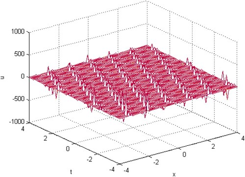3) Figure 1 illustrates the solution $u_1$.

Figure 1. Shape of Equation (32(32) $\begin{array}{rl}{u}_{1,2}(x,t)& =\pm \sqrt{({\alpha }^2+\text{β})(2\alpha -1)}\\ & \times \tan \left(\sqrt{\frac{{\alpha }^2+\text{β}}{2}}(\alpha x+\text{β}t+\zeta +\mu )\right)\end{array}$(32) ) for α = 1.8, β = 2, ζ =0.7, μ = 0.4.

Family II. At $({\alpha }^2+\text{β})<0$, swapping Equations (29(29) $\begin{array}{rl}b& =0,\end{array}$(29) )–(31(31) $\begin{array}{rl}a& =\pm \sqrt{\frac{1}{2(2\alpha -1)}},\end{array}$(31) ) and (18(18) $\begin{array}{r}u(x,t)={\mathrm{e}}^{\mathrm{i}}\eta u\left(\eta \right);v(x,t)=v\left(\eta \right);\eta =\alpha x+\text{β}t+\zeta ,\end{array}$(18) ) into Equations (12(12) $\begin{array}{rl}\chi \left(\eta \right)& =\left(\frac{-b}{2a}-\frac{\sqrt{4ac-b^2}}{2a}\right.\\ & {\left.\times \coth \left(\frac{(1-r)\sqrt{b^2-4ac}}{2}(\eta +\mu )\right)\right)}^{1/\left(1-r\right)}\end{array}$(12) ) and (13(13) $\begin{array}{rl}\chi \left(\eta \right)& =\left(\frac{-b}{2a}-\frac{\sqrt{4ac-b^2}}{2a}\right.\\ & {\left.\times \tanh \left(\frac{(1-r)\sqrt{b^2-4ac}}{2}(\eta +\mu )\right)\right)}^{1/\left(1-r\right)}\end{array}$(13) ), yields (34) $\begin{array}{rl}{u}_{5,6}(x,t)& =\pm \sqrt{-({\alpha }^2+\text{β})(2\alpha -1)}\tanh \\ & \times \left(\sqrt{-\frac{{\alpha }^2+\text{β}}{2}}(\alpha x+\text{β}t+\zeta +\mu )\right)\end{array}$(34) and (35) $\begin{array}{rl}{u}_{7,8}(x,t)& =\pm \sqrt{-({\alpha }^2+\text{β})(2\alpha -1)}\coth \\ & \times \left(\sqrt{-\frac{{\alpha }^2+\text{β}}{2}}(\alpha x+\text{β}t+\zeta +\mu )\right).\end{array}$(3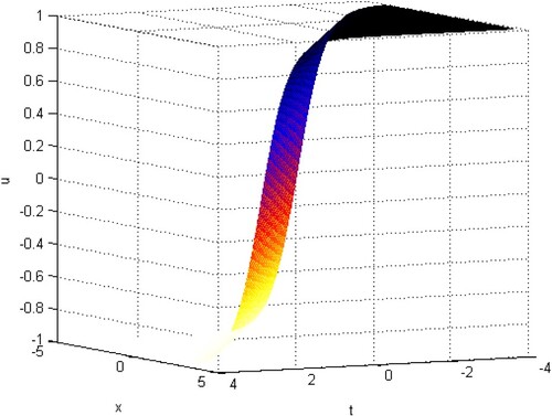5) Figure 2 illustrates the solution $u_5$.

Figure 2. Shape of Equation (34(34) $\begin{array}{rl}{u}_{5,6}(x,t)& =\pm \sqrt{-({\alpha }^2+\text{β})(2\alpha -1)}\tanh \\ & \times \left(\sqrt{-\frac{{\alpha }^2+\text{β}}{2}}(\alpha x+\text{β}t+\zeta +\mu )\right)\end{array}$(34) ) for α = 1.6, $\text{β}=-3$, ζ =0.7, μ = 0.4.

Family III. At b = 0 and c = 0: (36) $\begin{array}{r}{u}_{9,10}(x,t)={\left(\mp \sqrt{\frac{1}{2(2\alpha -1)}}\left(\alpha x+\text{β}t+\zeta +\mu \right)\right)}^{-1}.\end{array}$(36) In summary, it has been noted that the exact solutions for the LS system were achieved in the explicit forms, which have an important contribution in the nonlinear optical systems, bio-physics, plasma physics and hydrodynamics.

Remark 3.1

Using Equations (32(32) $\begin{array}{rl}{u}_{1,2}(x,t)& =\pm \sqrt{({\alpha }^2+\text{β})(2\alpha -1)}\\ & \times \tan \left(\sqrt{\frac{{\alpha }^2+\text{β}}{2}}(\alpha x+\text{β}t+\zeta +\mu )\right)\end{array}$(32) )–(36(36) $\begin{array}{r}{u}_{9,10}(x,t)={\left(\mp \sqrt{\frac{1}{2(2\alpha -1)}}\left(\alpha x+\text{β}t+\zeta +\mu \right)\right)}^{-1}.\end{array}$(36) ) and (18(18) $\begin{array}{r}u(x,t)={\mathrm{e}}^{\mathrm{i}}\eta u\left(\eta \right);v(x,t)=v\left(\eta \right);\eta =\alpha x+\text{β}t+\zeta ,\end{array}$(18) ), then the new explicit exact solution to LS system gained for Equation (17(17) $\begin{array}{rl}& \mathrm{i}{u}_t+u_{xx}-uv=0,\\ & v_t+v_x+(\mid u{\mid }^2{)}_x=0,\end{array}$(17) ).

Remark 3.2

Implementing Equation (16(16) $\begin{array}{r}{\chi }_n\left(\eta \right)={\left(\frac{-c{\mathrm{\Lambda }}_1+a{\mathrm{\Lambda }}_2{\left({\chi }_{n-1}\left(\eta \right)\right)}^{1-r}}{b{\mathrm{\Lambda }}_1+a{\mathrm{\Lambda }}_2+a{\mathrm{\Lambda }}_1{\left({\chi }_{n-1}\left(\eta \right)\right)}^{1-r}}\right)}^{1/\left(1-r\right)},\end{array}$(16) ) for $u_i(x,t)$ $(i=1,2,\dots ,10)$ one time, generates new infinite solutions orf Equation (17(17) $\begin{array}{rl}& \mathrm{i}{u}_t+u_{xx}-uv=0,\\ & v_t+v_x+(\mid u{\mid }^2{)}_x=0,\end{array}$(17) ).

Remark 3.3

The main advantages of RB sub-ODE method over other exiting methods is that it gives many new exact travelling wave solutions with additional free parameters. Remark 3.2 shows that RB sub-ODE method yields an infinite solutions of the LS system. Furthermore, this method is easy, direct and efficacious to get exact solutions for various types of NPDEs.

4. The random Riccati–Bernoulli sub-RODE technique

We consider RB sub-ODE scheme to solve the random models such as random differential equations (RDEs) or random partial differential equations (RPDEs). The randomness input is found by using the random wave transformation due to the random speed of the localized random wave solution of the problem. The important sense for using this method are the consistency, stability and the convergence theorems and so, we can state the stability theory in the next section.

4.1. The bi-random Riccati–Bernoulli sub-RODE technique

In this section, we consider the random case of the RB sub-RODE scheme. Recall the PDE (37) $P(\chi ,{\chi }_t,{\chi }_x,{\chi }_{tt},{\chi }_{xx},\dots )=0.$(37) Utilizing the random wave transformation (38) $\chi (x,t)=u\left(\eta \right),\eta =\alpha x+\text{β}t,$(38) where α and β are random variables. This means that the localized random wave solution $\chi \left(\eta \right)$ travels with random speed α, whereas β is a positive random variable. Equation (38(38) $\chi (x,t)=u\left(\eta \right),\eta =\alpha x+\text{β}t,$(38) ), converts Equation (37(37) $P(\chi ,{\chi }_t,{\chi }_x,{\chi }_{tt},{\chi }_{xx},\dots )=0.$(37) ) into RODE: (39) $H(\chi ,{\chi }^{\prime },{\chi }^{″},{\chi }^{‴},\dots )=0.$(39) Similarly to the deterministic case, the random solution of Equation (39(39) $H(\chi ,{\chi }^{\prime },{\chi }^{″},{\chi }^{‴},\dots )=0.$(39) ) obeys (40) ${\chi }^{\prime }=a{\chi }^{2-r}+b\chi +c{\chi }^r,$(40) where a, b, c and r are constants. We can also get random Equations (41(41) $\begin{array}{rl}{\chi }^{″}& =ab(3-r){\chi }^{2-r}+a^2(2-r){\chi }^{3-2r}+r{c}^2{\chi }^{2r-1}\\ & +bc(r+1){\chi }^r+(2ac+b^2)\chi ,\end{array}$(41) ) and (42(42) $\begin{array}{rl}{\chi }^{‴}& =\left(ab\right(3-r\left)\right(2-r){\chi }^{1-r}+a^2(2-r\left)\right(3-2r){\chi }^{2-2r}\\ & +r(2r-1)c^2{\chi }^{2r-2}+bcr(r+1){\chi }^{r-1}\\ & +(2ac+b^2)){\chi }^{\prime }.\end{array}$(42) ) like as Equations (5(5) $\begin{array}{rl}{\chi }^{″}& =ab(3-r){\chi }^{2-r}+a^2(2-r){\chi }^{3-2r}+r{c}^2{\chi }^{2r-1}\\ & +bc(r+1){\chi }^r+(2ac+b^2)\chi ,\end{array}$(5) ) and (6(6) $\begin{array}{rl}{\chi }^{‴}& =\left(ab\right(3-r\left)\right(2-r){\chi }^{1-r}+a^2(2-r\left)\right(3-2r){\chi }^{2-2r}\\ & +r(2r-1)c^2{\chi }^{2r-2}+bcr(r+1){\chi }^{r-1}\\ & +(2ac+b^2)){\chi }^{\prime }.\end{array}$(6) ). From Equation (40(40) ${\chi }^{\prime }=a{\chi }^{2-r}+b\chi +c{\chi }^r,$(40) ) and by directly calculating, we get (41) $\begin{array}{rl}{\chi }^{″}& =ab(3-r){\chi }^{2-r}+a^2(2-r){\chi }^{3-2r}+r{c}^2{\chi }^{2r-1}\\ & +bc(r+1){\chi }^r+(2ac+b^2)\chi ,\end{array}$(41) (42) $\begin{array}{rl}{\chi }^{‴}& =\left(ab\right(3-r\left)\right(2-r){\chi }^{1-r}+a^2(2-r\left)\right(3-2r){\chi }^{2-2r}\\ & +r(2r-1)c^2{\chi }^{2r-2}+bcr(r+1){\chi }^{r-1}\\ & +(2ac+b^2)){\chi }^{\prime }.\end{array}$(42) To obtain the random travelling wave solutions for Equation (37(37) $P(\chi ,{\chi }_t,{\chi }_x,{\chi }_{tt},{\chi }_{xx},\dots )=0.$(37) ), we follows similarly step 3 in deterministic case.

Finally, we can classify all cases of random solutions for the Random RB Equation (40(40) ${\chi }^{\prime }=a{\chi }^{2-r}+b\chi +c{\chi }^r,$(40) ) like as the same cases in deterministic case (Cases 1–6), but in the random case we must add for all cases the important condition as follows: α and β are bounded random variables. i.e. ${\text{β}}_1<\text{β}<{\text{β}}_2$; ${\alpha }_1<\alpha <{\alpha }_2$; ${\text{β}}_1$,${\text{β}}_2$, ${\alpha }_1$,${\alpha }_2$  are positive constants.

4.2. The stability for bi-random Riccati–Bernoulli sub-ODE solutions

Definition 1

A real random variable X defined on the probability space (Ω, $ϝ$, $P$) and satisfying: $\mathrm{E}\left[|X{|}^2\right]<\mathrm{\infty }$ is called second order random variable ($2.r.v$), $\mathrm{E}\left[\right]$ represents the expectation value operator.

If we consider the stability for the solutions that obtained by the RB sub-ODE scheme in random case, then the main condition is that all random variable must be bounded. We can summaries our stability conditions for the random solutions in the following theorem.

Theorem 4.1

[42, 43]

The random solutions obtained by bi-Random RB sub-ODE technique is stable with respect the main condition that, the random wave transformation parameters are second order random variables.

We will discuss this theorem through the following application.

5. Solutions of long–short-wave interaction system using bi-Random Riccati–Bernoulli sub-RODE method

Recall LS system (17(17) $\begin{array}{rl}& \mathrm{i}{u}_t+u_{xx}-uv=0,\\ & v_t+v_x+(\mid u{\mid }^2{)}_x=0,\end{array}$(17) ) and using random travelling wave transformation (43) $u(x,t)=e^{i\eta }u\left(\eta \right),,v(x,t)=v\left(\eta \right)\eta =\alpha x+\text{β}t+\zeta .$(43) where α and β are random variables.

Equation (17(17) $\begin{array}{rl}& \mathrm{i}{u}_t+u_{xx}-uv=0,\\ & v_t+v_x+(\mid u{\mid }^2{)}_x=0,\end{array}$(17) ) transforms into the following RODEs, using (43(43) $u(x,t)=e^{i\eta }u\left(\eta \right),,v(x,t)=v\left(\eta \right)\eta =\alpha x+\text{β}t+\zeta .$(43) ): (44) $\begin{array}{rl}& u^{″}-uv-({\alpha }^2+\text{β})u=0,\end{array}$(44) (45) $\begin{array}{rl}& (1-2\alpha )v^{\prime }+2u{u}^{\prime }=0,\end{array}$(45) where α and β are random variables. Now we follow exactly the same procedure in Section 3, which yields the same forms of solutions in random case. Here, we take in consideration only one random case, whereas the other cases follow likewise.

The case study. At $\left(\mathbb{E}\right[{\alpha }^2]+\mathbb{E}[\text{β}\left]\right)>0$, the exact random travelling wave solutions of Equation (17(17) $\begin{array}{rl}& \mathrm{i}{u}_t+u_{xx}-uv=0,\\ & v_t+v_x+(\mid u{\mid }^2{)}_x=0,\end{array}$(17) ): (46) $\begin{array}{rl}{u}_{1,2}(x,t)& =\pm \sqrt{({\alpha }^2+\text{β})(2\alpha -1)}\tan \\ & \times \left(\sqrt{\frac{{\alpha }^2+\text{β}}{2}}(\alpha x+\text{β}t+\zeta +\mu )\right)\end{array}$(46) and (47) $\begin{array}{rl}{u}_{3,4}(x,t)& =\pm \sqrt{({\alpha }^2+\text{β})(2\alpha -1)}\cot \\ & \times \left(\sqrt{\frac{{\alpha }^2+\text{β}}{2}}(\alpha x+\text{β}t+\zeta +\mu )\right),\end{array}$(47) α and β are random variables with $\mathbb{E}\left[{\alpha }^2\right]<\mathrm{\infty }$, $\mathbb{E}\left[\text{β}\right]<\mathrm{\infty }$ and ζ, μ are arbitrary constants.

The solutions $u_1,u_2,u_3$ and $u_4$ for some random distributions are depicted in Figures 3–6. Namely, in this section we have deal with random travelling wave when the coefficients be random variables. This means that our solutions are stochastic process solutions. Therefore, we can get the statistical properties of the random solutions such as the mean, variance, etc. Also, physically we can forecast by any disturbances that may be occurred when we study any applied problem. In this work, we discussed the mean random solutions behaviour as shown in Figures 3–6 for the random solutions $u_1,u_2,u_3$ and $u_4$ under Beta, Poisson and exponential statistical distributions.

Figure 3. Shape of $E\left[u\right]=E\left[u1\right(x,t\left)\right]$ for the random LS system.

Figure 4. Shape of $E\left[u\right]=E\left[u2\right(x,t\left)\right]$ for the random LS system.

Figure 5. Shape of $E\left[u\right]=E\left[u3\right(x,t\left)\right]$ for the random LS system.

Figure 6. Shape of $E\left[u\right]=E\left[u4\right(x,t\left)\right]$ for the random LS system.

6. Conclusions

In this article, some new travelling wave solutions for the LS system is successfully obtained, using the RB sub-ODE method. The calculations show that these methods are efficient, powerful and robust to get vital solutions in a unified and more general way. Furthermore, some bi-random variables and some random distributions are used in random case corresponding to the LS system. Indeed, the stability for bi-Random RB sub-ODE solutions is given. We observe that the proposed method is straightforward and can be applied for deterministic and stochastic cases for many other NPDEs in applied science. Finally, a new combination between two vital branches of science, namely partial differential equations and applied statistics is introduced, which give a validity of so interesting applications in the forthcoming papers.

Disclosure statement

No potential conflict of interest was reported by the author(s).

References

- Abdelrahman MAE, Kunik M. The ultra-relativistic Euler equations. Math Meth Appl Sci. 2015;38:1247–1264.
- Abdelrahman MAE. Global solutions for the ultra- relativistic Euler equations. Nonlinear Anal. 2017;155:140–162.
- Abdelrahman MAE. On the shallow water equations. Z Naturforsch A. 2017;72(9):873–879.
- Abdelrahman MAE. Cone-grid scheme for solving hyperbolic systems of conservation laws and one application. Comp Appl Math. 2018;37(3):3503–3513.
- Abdelrahman MAE, Hassan SZ, Inc M. The coupled nonlinear Schrödinger-type equations. Modern Phys Lett B. 2020;34:2050078. doi:10.1142/s0217984920500785.
- Razborova P, Ahmed B, Biswas A. Solitons, shock waves and conservation laws of Rosenau-KdV-RLW equation with power law nonlinearity. Appl Math Inf Sci. 2014;8(2): 485–491.
- Yaslan HC, Girgin E. New exact solutions for the conformable space-time fractional KdV, CDG, (2+1)- dimensional CBS and (2+1)-dimensional AKNS equations. J Taibah Sci. 2019;13(1):1–8.
- Bhrawy AH. An efficient Jacobi pseudospectral approximation for nonlinear complex generalized Zakharov system. Appl Math Comput. 2014;247:30–46.
- Abdelrahman MAE, Sohaly MA. On the new wave solutions to the MCH equation. Indian J Phys. 2019;93:903–911. (2018).
- Abdelrahman MAE, Hassan SZ. A Riccati–Bernoulli sub-ODE method for some nonlinear evolution equations. Int J Nonlinear Sci Numerical Simul. 2019;20(3–4):303–313.
- Abdelrahman MAE, Sohaly MA. The development of the deterministic nonlinear PDEs in particle physics to stochastic case. Results Phys. 2018;9:344–350.
- Kumar D, Agarwal RP, Singh J. A modified numerical scheme and convergence analysis for fractional model of Lienard's equation. J Comput Appl Math. 2018;339:405–413.
- Kumar D, Singh J, Baleanu D. A new numerical algorithm for fractional Fitzhugh–Nagumo equation arising in transmission of nerve impulses. Nonlinear Dyn. 2018;91: 307–317.
- Li T, Pintus N, Viglialoro G. Properties of solutions to porous medium problems with different sources and boundary conditions. Z Angew Math Phys. 2019;70:86.
- Wazwaz AM. The tanh method for travelling wave solutions of nonlinear equations. Appl Math Comput. 2004;154:714–723.
- Fan E, Zhang H. A note on the homogeneous balance method. Phys Lett A. 1998;246:403–406.
- Aminikhad H, Moosaei H, Hajipour M. Exact solutions for nonlinear partial differential equations via Exp-function method. Numer Methods Partial Differ Equ. 2009;26:1427–1433.
- Yang XF, Deng ZC, Wei Y. A Riccati-Bernoulli sub-ODE method for nonlinear partial differential equations and its application. Adv Differ Equ. 2015;1:117–133.
- Abdelrahman MAE. A note on Riccati-Bernoulli sub-ODE method combined with complex transform method applied to fractional differential equations. Nonlinear Engin Model Appl. 2018;7(4). Available from: https://doi.org/10.1515/nleng-2017-0145.
- Hassan SZ, Abdelrahman MAE. Solitary wave solutions for some nonlinear time fractional partial differential equations. Pramana J Phys. 2018;91:67.
- Wazwaz AM. Exact solutions to the double sinh-Gordon equation by the tanh method and a variable separated ODE. Method Comput Math Appl. 2005;50:1685–1696.
- He JH. Variational principles for some nonlinear partial differential equations with variable coefficients. Chaos Solitons Fractals. 2004;19(4):847–851.
- He JH. Application of homotopy perturbation method to nonlinear wave equations. Chaos Solitons Fractals. 2005;26:695–700.
- Wang ML, Zhang JL, Li XZ. The (G′G)- expansion method and travelling wave solutions of nonlinear evolutions equations in mathematical physics. Phys Lett A. 2008;372:417–423.
- Zhang S, Tong JL, Wang W. A generalized (G′G)- expansion method for the mKdv equation with variable coefficients. Phys Lett A. 2008;372:2254–2257.
- Dai CQ, Zhang JF. Jacobian elliptic function method for nonlinear differential difference equations. Chaos Solutions Fractals. 2006;27:1042–1049.
- Eslami M. Trial solution technique to chiral nonlinear Schrodinger's equation in (1+2)-dimensions. Nonlinear Dyn. 2016;85:813–816.
- Kumar D, Singh J, Purohit SD, et al. A hybrid analytical algorithm for nonlinear fractional wave-like equations. Math Model Nat Phenom. 2019;14:304.
- Bhatter S, Mathur A, Kumar D, et al. Fractional modified Kawahara equation with Mittag-Leffler law. Chaos Solitons Fractals. 2020;131:109508.
- Goswami A, Singh J, Kumar D. An efficient analytical approach for fractional equal width equations describing hydro-magnetic waves in cold plasma. Physica A. 2019;524:563–575.
- Bhatter S, Mathur A, Kumar D, et al. A new analysis of fractional Drinfeld-Sokolov-Wilson model with exponential memory. Physica A. 2020;537:122578.
- Singh J, Kilicman A, Kumar D, et al. Numerical study for fractional model of nonlinear predator-prey biological population dynamical system. Thermal Sci. 2019;23(6):S2017–S2025.
- Yüzbasi S. Numerical solutions of fractional Riccati type differential equations by means of the Bernstein polynomials. Appl Math Comput. 2013;219:6328–6343.
- Lakestani M, Dehghan M. Numerical solution of Riccati equation using the cubic B-spline scaling functions and Chebyshev cardinal functions. Comput Phys Commun. 2010;181:957–966.
- Yüzbasi S. A collocation approach to solve the Riccati-type differential equation systems. Int J Comput Math. 2013;89:2180–2197.
- File G, Aga T. Numerical solution of quadratic Riccati differential equations. Egyptian J Basic Appl Sci. 2016;3:392–397.
- Yüzbasi S. A numerical approach for solving the high-order linear singular differential-difference equations. Comput Math Appl. 2011;62:2289–2303.
- Wang ML, Wang YM, Zhang JL. The periodic wave solutions for two systems of nonlinear wave equations. Chin Phys. 2003;12:1341–1348.
- Kloeden PE, Platen E. Numerical solution of stochastic differential equations. Springer, New York, 1992.
- Sohaly M. Mean square convergent three and five points finite difference scheme for stochastic parabolic partial differential equations. Electron J Math Anal Appl. 2014;2(1):164–171.
- Yassen M, Sohaly M, Elbaz I. Random Crank-Nicolson scheme for random heat equation in mean square sense. Amer J Comput Math. 2016;6:66–73.
- Cortes J-C, Romero JV, Roselló MD. Solving random boundary heat model using the finite difference method under mean square convergence. Comput Math Methods. 2019;1(3):e1026.
- Sohaly MA. Random difference scheme for diffusion advection model. Adv Differ Equ. 2019;2019(1):54.