
 ?Mathematical formulae have been encoded as MathML and are displayed in this HTML version using MathJax in order to improve their display. Uncheck the box to turn MathJax off. This feature requires Javascript. Click on a formula to zoom.
Abstract
In this study, we consider the third order nonlinear Schrödinger equation (TONSE) that models the wave pulse transmission in a time period less than one-trillionth of a second. With the help of the extended modified method, we obtain numerous exact travelling wave solutions containing sets of generalized hyperbolic, trigonometric and rational solutions that are more general than classical ones. Secondly, we construct the transformation groups which left the equations invariant and vector fields with the Lie symmetry groups approach. With the help of these vector fields, we obtain the symmetry reductions and exact solutions of the equation. The obtained group-invariant solutions are Jacobi elliptic function and exponential type. We discuss the dynamic behaviour and structure of the exact solutions for distinct solutions of arbitrary constants. Lastly, we obtain conservation laws of the considered equation by construing the complex equation as a system of two real partial differential equations (PDEs).
1. Introduction
It is observed that most of the physical phenomena occurring in nature are mathematically modelled by the evolution equations. However, we know from the empirical results that many important physical processes are the type of nonlinear evolution equations (NLEEs)
(1)
(1) [Citation1–7]. Well-known Korteweg-de Vries equation
(2)
(2) represents shallow water waves. Soliton which is a special solitary travelling wave -unchanged wave velocity and shape after interaction- is a generalized wave packet. For these reasons, a travelling wave solution is used not only in water wave theory, but also in optical communication. Solitons are derived from the sensitive interaction between nonlinear and dispersive terms.
It is desirable that travelling wave solution transmission in communication systems should be high speed [Citation8,Citation9]. For example, the -dimensional nonlinear Schrödinger equation (NLSE)
(3)
(3)
can be used to represent the transmission of optical pulses in optical fibres in the picosecond [Citation10]. It has been observed in both experimental and numerical simulations that higher order nonlinear terms and effects should be taken into consideration in order to make the transmission in Equation (Equation3
(3)
(3) ) faster (sub-picosecond or femtosecond). In this study, we will consider the third order equations
(4)
(4) from the hierarchy of the higher order NLSE given in [Citation8,Citation11–13]. Our main goal is to obtain exact analytical solutions of this equation. There are many methods in the literature to obtain the solutions of the nonlinear Schrödinger equations (NLSEs) and NLEEs. Some of them are listed in [Citation14–27].
Recently, the modified sub-equation extended method are introduced in [Citation28]. What makes this method interesting is that, unlike other methods, solutions include the generalized type of hyperbolic and trigonometric functions. This method has a finite series expansion form based on the balancing principle. Higher order NLSEs were taken into consideration by researchers in recent years [Citation11,Citation29–32]. However, to the best of our knowledge, the exact solutions that contain generalized hyperbolic and trigonometric functions of third-order NLS equations have not been studied. The lack of studies in the literature on the exact solutions of Equation (Equation4(4)
(4) ) motivated us. In order to overcome this deficiency, this method, which is very effective and practical for solving nonlinear differential equations in mathematical physics, was used to obtain the solutions of the equation under consideration. Another approach discussed in this study is Lie technique. In this algorithmic method based on the finding of transformation groups that leave the equation invariant, reduced equations and group invariant solutions can be obtained. In this study, the wave and group invariant solutions of Equation (Equation4
(4)
(4) ) will be investigated with the help of these two methods.
In the second section of the article, the reduction of Equation (Equation4(4)
(4) ) to the ordinary differential equation will be discussed. In the third section, the modified sub-equation extended method is presented and its application to Equation (Equation4
(4)
(4) ) is given. In Section 4, Lie groups method is employed to study Equation (Equation4
(4)
(4) ). Lie point symmetries and invariant solutions are obtained in Sections 5 and 6, respectively. In Section 7, the conservation laws are computed. The results and discussion are presented in the Section 8.
2. Mathematical model
In spite of the fact that Equation (Equation3(3)
(3) ) is successful in describing a great number of nonlinear effects, it may be necessary to modify the experimental conditions. Therefore, higher-order effects should be considered for the transmission of pulses to sub-picoseconds and femtoseconds which has a better performance on the transmitting information. The higher-order integrable NLS hierarchy can be presented as
(5)
(5) where
represents the normalized complex amplitude of the optical pulse envelope, asterisk represents the conjugation,
are real constant parameters, x denotes the propagation variable and, t denotes the transverse variable (time in a moving frame) [Citation11–13]. In this study, we will investigate the Equation (Equation4
(4)
(4) ) which we have obtained by taking
. In this section, we aim to simplify the Equation (Equation4
(4)
(4) ). Thus, we are seeking solutions of (Equation4
(4)
(4) ) with the following structure
(6)
(6) where
is the wave variable and
is an amplitude component of the soliton solution. Here v and κ are the velocity and frequency of the soliton, respectively. ϖ is the soliton wave number and, θ is the phase constant. If we use the transformation given by (Equation6
(6)
(6) ) in the Equation (Equation4
(4)
(4) ) and separate the real and imaginary parts, a pair of relations emerges. The real part equation gives
(7)
(7) and imaginary part equation reads
(8)
(8) Integrating Equation (Equation8
(8)
(8) ) once and setting the integration constant to zero, we obtain
(9)
(9) Equation (Equation7
(7)
(7) ) and (Equation9
(9)
(9) ) will be equivalent, provided that
Hence, one can find the following parametric constraints,
(10)
(10) Eventually, Equations (Equation7
(7)
(7) ) and (Equation9
(9)
(9) ) can be rearranged to be in the form
(11)
(11) In the next sections, solutions of the Equation (Equation11
(11)
(11) ) will be examined using the extended modified sub-equation method.
3. Basic ideas of the extended modified sub-equation method
Here, we present briefly the main steps of the extended modified sub-equation method for finding travelling wave solutions to NLEEs [Citation28]. Firstly, we consider the general NLEE of the type
(12)
(12) Using the wave transformation
we can rewrite Equation (Equation12
(12)
(12) ) as the following nonlinear ordinary differential equation (NLODE):
(13)
(13) Let us assume that the solution of ordinary differential equation (ODE) (Equation13
(13)
(13) ) can be written as a polynomial of
as follows:
(14)
(14) where
are constants which will be determined later.
in (Equation14
(14)
(14) ) satisfies the NLODE in the form
(15)
(15) The coefficient classifications and corresponding solution forms of (Equation15
(15)
(15) ) are as follows:
Case 1: If then
Case 2: If then
Case 3: If then
Case 4: If then
Case 5: If then
Case 6: If ,
and
then
Case 7: If then
Case 8: If then
Case 9: If then
Case 10: If ,
and
then
The generalized trigonometric and hyperbolic functions used in the families given above are defined as follows:
(16)
(16) In Equation (Equation16
(16)
(16) ), ς is an independent variable, r, p>0 constants are deformation parameters. n in (Equation14
(14)
(14) ) is a positive integer that can be determined by the balancing procedure constructed taking into account the highest order nonlinear terms and the highest order linear terms in the resulting equation. By using Equation (Equation14
(14)
(14) ) and Equation (Equation15
(15)
(15) ) into Equation (Equation13
(13)
(13) ), an equation consisting of the powers of
is obtained. With the determination of n, the coefficients of the equation rearranged according to the powers of
has to be equal to zero. Hence, we obtain an algebraic system of equations in terms of
. By determining these parameters and rewriting the Equation (Equation14
(14)
(14) ) using determined parameters, an analytic solution
is obtained, in a closed form.
4. Exact travelling wave solutions
In this section, we will obtain the analytical solutions for the amplitude of the travelling wave solutions by using the extended modified sub-equation method. Substituting into Equation (Equation11
(11)
(11) ) and balancing
with
yields n = 1. Therefore Equation (Equation11
(11)
(11) ) admits the use of
(17)
(17) Substituting Equation (Equation17
(17)
(17) ) into Equation (Equation11
(11)
(11) ) through Equation (Equation15
(15)
(15) ) and, collecting the coefficients of different powers of
, setting each coefficient to zero, we get the system of algebraic equations. By solving the resulting system with the help of Maple, the following results are achieved:
Set 1
After the huge calculations, we deduce the following relations between parameters appearing algebraic equations:
where
are arbitrary constants. We now can construct the exact solutions of Equation (Equation4
(4)
(4) ) easily for these parameters set through the classification cases which is given in Section 3.
Case 1: If then we have
(18)
(18)
Case 2: If then we obtain
Case 3: If then we yield
Case 4: If then one obtains
Case 5: If then we attain
(19)
(19)
Case 6: If ,
and
then we derive
Case 9: If then we construct
Case 10: If ,
and
then we get
Set 2
After some calculations, the following relations are obtained between the parameters in the system of algebraic equations:
where are arbitrary constants. According to classification cases for these parameters in Section 3, we can construct the exact solutions of Equation (Equation4
(4)
(4) ) as follows:
Case 1: If then
Case 2: If then
(20)
(20)
Case 3: If then
Case 4: If then
Case 5: If then
Case 6: If ,
and
then
Case 8: If then
Case 9: If then
(21)
(21)
5. Lie symmetries
We will apply Lie symmetry analysis for Equation (Equation4(4)
(4) ) [Citation33–38]. Firstly, we assume
(22)
(22) where u and v are real valued functions. If we substitute (Equation22
(22)
(22) ) into (Equation4
(4)
(4) ) and split up real and imaginary parts, we obtain
(23)
(23) For the system of the above equations, let us consider infinitesimal transformations which contain the essential information determining a one-parameter Lie group of transformations:
(24)
(24) with a small parameter
. The corresponding vector field for these transformations is
(25)
(25) When (Equation25
(25)
(25) ) vector field (or generator) is found, the transformation group of the equation or system considered is
The third prolongations formula
is
(26)
(26) where
are extended infinitesimal. Hence, system of equations (Equation23
(23)
(23) ) has following invariance conditions:
With the help of the obtained equation pair and the values of extended infinitesimals, we get an overdetermined system of PDEs. Solving overdetermined system of PDEs, one can obtain
(27)
(27) where
and
are arbitrary constants. Thus, the Lie algebra of infinitesimal symmetries of equations (Equation23
(23)
(23) ) is said to be spanned by the vector field
(28)
(28) It is easy to verify that
is closed under the Lie bracket. In fact, we have The commutator table is anti-symmetric with its diagonal elements all being zero as we have
(Table ) [Citation39,Citation40].
6. Symmetry reduction and invariant solutions
In this section, we will get the invariant solutions of system of Equation (Equation23(23)
(23) ). The corresponding characteristic equations are
(29)
(29) where
and φ are given by (Equation27
(27)
(27) ). Solving characteristic Equation (Equation29
(29)
(29) ), we will consider four cases of vector fields:
,
where are arbitrary real numbers different from zero.
Table 1. Commutator table of the vector fields of (Equation23(23) (23) ).
Case (i)
By solving the characteristic equation (Equation29(29)
(29) ) for the generator
, similarity variables are obtained as follows:
(30)
(30) where ρ and F, G are new independent and dependent variables, respectively. Substituting (Equation30
(30)
(30) ) into (Equation23
(23)
(23) ), the following similarity reduction can be obtained:
(31)
(31)
(32)
(32) where
denotes derivative with respect to ρ. Hence, solution of Equation (Equation4
(4)
(4) ) can be written as
(33)
(33) where
are solutions of (Equation31
(31)
(31) ) and (Equation32
(32)
(32) ).
Specially, let us choose in Equation (Equation31
(31)
(31) ) and Equation (Equation32
(32)
(32) ). By solving the equation obtained by taking the integral of the Equation (Equation32
(32)
(32) ) and the equation obtained from the Equation (Equation31
(31)
(31) ), we obtain
where JacobiSN is the Jacobi elliptic function. In this case, solution of (Equation4
(4)
(4) ) can be obtained as
Case (ii)
If the characteristic equation is generated according to and solved, similarity variables are obtained as follows
(34)
(34) where γ and J, K are new variables. Using the expressions given in (Equation34
(34)
(34) ) in the system of Equations (Equation23
(23)
(23) ), similarity reduction can be obtained as follows
(35)
(35)
(36)
(36) where a prime denotes differentiation with respect to γ. Equation (Equation36
(36)
(36) ) has the solution
(37)
(37) where
is arbitrary constant. Substituting (Equation36
(36)
(36) ) into (Equation35
(35)
(35) ) and solving, we get
(38)
(38) where
is arbitrary constant. From (Equation22
(22)
(22) ), (Equation34
(34)
(34) ), (Equation37
(37)
(37) ) and (Equation38
(38)
(38) ), the solution of Equation (Equation4
(4)
(4) ) is
Case (iii)
In this case, we deal with the linear combination of and
. Solving the corresponding characteristic equation, we have
(39)
(39) where P and Q are new independent variables of new independent variable ζ. According to new variables given in (Equation39
(39)
(39) ), we have following reduced equations:
(40)
(40)
(41)
(41) where
denotes differentiation with respect to ζ. Corresponding solution of Equation (Equation4
(4)
(4) ) can be presented as
(42)
(42) where ζ is given by (Equation39
(39)
(39) ) and
is solutions of (Equation40
(40)
(40) ) and (Equation41
(41)
(41) ) equations.
Specially, let us choose and
in Equation (Equation40
(40)
(40) ) and Equation (Equation41
(41)
(41) ), by solving the equation obtained by taking the integral of the Equation (Equation41
(41)
(41) ) and the equation obtained from the Equation (Equation40
(40)
(40) ), we obtain
where JacobiSN is the Jacobi elliptic function. In this case, solution of the Equation (Equation4
(4)
(4) ) can be expressed in term of original variables as
Case (iv)
Solving the characteristic equation (Equation29(29)
(29) ) for the generator
, we obtain following similarity variables:
(43)
(43) where σ and H, W are new variables. Substituting (Equation43
(43)
(43) ) into (Equation23
(23)
(23) ), we get the reduced equations as follows
(44)
(44)
(45)
(45) where
denotes differentiation with respect to σ. Thus the solution of Equation (Equation4
(4)
(4) ) can be given as
(46)
(46) where σ is given by (Equation43
(43)
(43) ) and
is solutions of (Equation44
(44)
(44) ) and (Equation45
(45)
(45) ) equations.
The one parameter groups generated by the
are given in the following table. The entries give the transformed point
:
We observe that the Lie groups
and
corresponds to the dependent variable, space and time translation,respectively. If
and
are any functions, then their transform by
is
which should be expressed in terms of
. Therefore
are transformed functions in this particular case.
7. Conservation laws
Consider a kth-order system of PDEs
(47)
(47) with two independent variables
and two dependent variables
. Let
,
, denote the collections of lth-order partial derivatives given with
, in terms of total derivative operator
(48)
(48) Using the familiar consequence that the Euler-Lagrange operator eliminates a total divergence, we employ the invariance and multiplier approach for determining conserved densities and fluxes. Firstly, if
is a conserved vector corresponding to a conservation law, then a total space-time divergence expression vanishes on the solutions of the system (Equation47
(47)
(47) ),
(49)
(49) A multiplier
has the property that
(50)
(50) or
(51)
(51) hold identically for some conserved vector
. The determining equation for the multiplier M is[33]
(52)
(52) where Ξ is the Euler operator. Thus, the multipliers can be determined by using (Equation52
(52)
(52) ). Then the corresponding conserved vectors can be constructed. There are several approaches to this, where the better-known approach is the homotopy formula [Citation41–43]. If the real and imaginary parts of the equation obtained by substituting q = u + iv into (Equation4
(4)
(4) ) are separated, the following equation pair is obtained:
(53)
(53) As a result of detailed calculations, it can be seen that if
with
the multipliers M with the corresponding densities
of the above system with
being the densities of (Equation4
(4)
(4) ) can be obtained.
According to the conserved densities obtained above, it is seen that linear momentum, power or Hamiltonian are not conserved. Here, we avoid any physical interpretation because the densities we obtain above are unusual [Citation44].
8. Conclusion
In this work, we considered the TONSE which enables studies and advances in the speed of information transmission that plays a major role in fields such as ultrashort pulses, optical fibre, applied physics, communication system, etc… To contribute to the studies of the higher order Schrödinger equation and the special cases of this equation in the literature [Citation31,Citation32,Citation45–47], we considered Equation (Equation4(4)
(4) ). This equation was considered in [Citation29,Citation30] for
and the authors studied the non autonomous characteristics of the W-shaped solitons and have modified the Darboux transformation method to find rational solutions of the equation of the first and second orders, respectively. As far as we know, the exact solutions of this equation, which include generalized hyperbolic and trigonometric functions, were investigated for the first time in this research. We believe that the solutions we have obtained are new. One of the advantages of the applied method is that it contains more general solutions than most of the methods in the literature. The results obtained by the application of this method have shown that this method is effective, strong and applicable to other problems in mathematical physics.
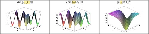
Moreover, for better understanding the dynamics of these results, we demonstrated graphs of real-imaginary parts and modulus of some of them by giving appropriate values to the parameters which facilitate to recognize the physical phenomena of this nonlinear mode in Figure –. The solution domain was chosen as in all illustrations. The modulus of
demonstrated periodic solution in Figure . The modulus of
and
describe rational soliton and optical dark travelling wave solutions in Figure and , respectively. The modulus part of
demonstrated singular periodic solution in Figure . In Section 5, we applied Lie classical method to considered equation to obtain the group-invariant solutions. The vector fields, symmetry reductions, transformation groups, and group-invariant solutions based on the Lie group approach were obtained. Finally, we constructed conservation laws of Equation (Equation4
(4)
(4) ) and obtained two conserved densities. The conservation laws that we obtain can be used in the stability analysis of solutions and in numerical schemes. In future studies, the conformable fractional derivative and the fractional modified sub-equation extended method for the generalized hyperbolic and trigonometric functions can be considered to obtain new solutions for the NLSEs. We believe that this study might be important for researchers specializing in the construction of the transmission media and more specifically optical fibres may have the opportunity to build new optical fibres, including waves, that adapt to the types of signals we want to propagate. We hope that these results are going to be very useful in future research.
Figure 1. Profile of solution for Set 1 when
in Equation (Equation18
(18)
(18) ).
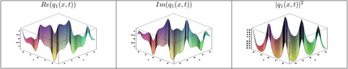
Figure 2. Profile of solution for Set 1 when
in Equation (Equation19
(19)
(19) ).
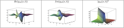
Figure 3. Profile of solution for Set 2 when
in Equation (Equation20
(20)
(20) ).
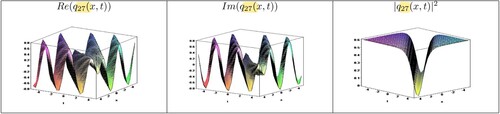
Figure 4. Profile of solution for Set 2 when
in Equation (Equation21
(21)
(21) ).
Disclosure statement
No potential conflict of interest was reported by the author(s).
References
- Hasegawa A, Tappert F. Transmission of stationary nonlinear optical pulses in dispersive dielectric fibers. I. Anomalous dispersion. Appl Phys Lett. 1973;23(3):142–144.
- Hasegawa A, Tappert F. Transmission of stationary nonlinear optical pulses in dispersive dielectric fibers. II. Normal dispersion. Appl Phys Lett. 1973;23(4):171–172.
- Bulut H, Sulaiman TA, Baskonus HM, et al. Optical solitons and other solutions to the conformable space–time fractional Fokas–Lenells equation. Optik. 2018;172:20–27.
- Arshed S, Biswas A, Abdelaty M, et al. Optical soliton perturbation for Gerdjikov–Ivanov equation via two analytical techniques. Chinese J Phys. 2018;56(6):2879–2886.
- Li BQ, Sun JZ, Ma YL. Soliton excitation for a coherently coupled nonlinear Schrödinger system in optical fibers with two orthogonally polarized components. Optik. 2018;175:275–283.
- Guan X, Liu W, Zhou Q, et al. Some lump solutions for a generalized (3+1)-dimensional Kadomtsev–Petviashvili equation. Appl Math Comput. 2020;366:124757.
- Guan X, Zhou Q, Liu W. Lump and lump strip solutions to the (3+1)-dimensional generalized Kadomtsev-Petviashvili equation. Eur Phys J Plus. 2019;134(7):371.
- Liu X, Triki H, Zhou Q, et al. Analytic study on interactions between periodic solitons with controllable parameters. Nonlinear Dyn. 2018;94(1):703–709.
- Liu W, Yu W, Yang C, et al. Analytic solutions for the generalized complex GinzburgoLandau equation in fiber lasers. Nonlinear Dyn. 2017;89(4):2933–2939.
- Agrawal GP. 1995. Nonlinear fiber optics. Academic, New York.
- Huang QM, Gao YT, Hu L. Breather-to-soliton transition for a sixth-order nonlinear Schrödinger equation in an optical fiber. Appl Math Lett. 2018;75:135–140.
- Wang L, Zhang JH, Wang ZQ, et al. Breather-to-soliton transitions, nonlinear wave interactions, and modulational instability in a higher-order generalized nonlinear Schrödinger equation. Phys Rev E. 2016;93(1):012214.
- Chowdury A, Ankiewicz A, Akhmediev N. Moving breathers and breather-to-soliton conversions for the Hirota equation. Proc R Soc A. 2015;471(2180):20150130.
- Cheemaa N, Younis M. New and more general traveling wave solutions for nonlinear Schrödinger equation. Waves Random Complex Media. 2016;26(1):30–41.
- Seadawy AR, Lu D. Bright and dark solitary wave soliton solutions for the generalized higher order nonlinear Schrödinger equation and its stability. Results Phys. 2017;7:43–48.
- Marin M, Vlase S, Ellahi R, et al. On the partition of energies for the backward in time problem of thermoelastic materials with a dipolar structure. Symmetry. 2019;11(7):863.
- Seadawy AR. Modulation instability analysis for the generalized derivative higher order nonlinear Schrödinger equation and its the bright and dark soliton solutions. J Electromagn Waves Appl. 2017;31(14):1353–1362.
- Biswas A, Yildirim Y, Yasar E, et al. Optical soliton perturbation with Gerdjikov–Ivanov equation by modified simple equation method. Optik. 2018;157:1235–1240.
- Manafian J. Optical soliton solutions for Schrödinger type nonlinear evolution equations by the tan(φ(ξ)/2)-expansion method. Optik. 2016;127(10):4222–4245.
- Marin M. Lagrange identity method for microstretch thermoelastic materials. J Math Anal Appl. 2010;363(1):275–286.
- Nasreen N, Seadawy AR, Lu D, et al. Solitons and elliptic function solutions of higher-order dispersive and perturbed nonlinear Schrodinger equations with the power-law nonlinearities in non-Kerr medium. Eur Phys J Plus. 2019;134:485.
- Seadawy AR. Approximation solutions of derivative nonlinear Schrodinger equation with computational applications by variational method. Eur Phys J Plus. 2015;130(9):182.
- Marin MI, Agarwal RP, Mahmoud SR. Nonsimple material problems addressed by the Lagrange's identity. Bound Value Probl. 2013;2013(1):135.
- Yan Y, Liu W. Stable transmission of solitons in the complex cubic-quintic Ginzburg-Landau equation with nonlinear gain and higher-order effects. Appl Math Lett. 2019;98:171–176.
- Liu W, Zhang Y, Wazwaz AM, et al. Analytic study on triple-S, triple-triangle structure interactions for solitons in inhomogeneous multi-mode fiber. Appl Math Comput. 2019;361:325–331.
- Marin M, Ellahi R, Chirilă A. On solutions of Saint-Venant's problem for elastic dipolar bodies with voids. Carpathian J Math. 2017;33(2):219–232.
- Marin M, Bhatti MM. Head-on collision between capillary–gravity solitary waves. Bound Value Probl. 2020;2020(1):1–18.
- Yépez-Martínez H, Rezazadeh H, Souleymanou A, et al. The extended modified method applied to optical solitons solutions in birefringent fibers with weak nonlocal nonlinearity and four wave mixing. Chinese J Phys. 2019;58:137–150.
- Zhang X, Zhao YC, Qi FH, et al. Characteristics of nonautonomous W-shaped soliton and Peregrine comb in a variable-coefficient higher-order nonlinear Schrödinger equation. Superlattices Microstruct. 2016;100:934–940.
- Ankiewicz A, Soto-Crespo JM, Akhmediev N. Rogue waves and rational solutions of the Hirota equation. Phys Rev E. 2010;81(4):046602.
- Arshad M, Seadawy AR, Lu D. Exact bright–dark solitary wave solutions of the higher-order cubic–quintic nonlinear Schrödinger equation and its stability. Optik. 2017;138:40–49.
- Wang XB, Zhang TT, Dong MJ. Dynamics of the breathers and rogue waves in the higher-order nonlinear Schrödinger equation. Appl Math Lett. 2018;86:298–304.
- Olver PJ. Applications of Lie groups to differential equations. Vol. 107. New York: Springer Science Business Media; 2000.
- Ibragimov NH. A practical course in differential equations and mathematical modelling: classical and new methods. Nonlinear mathematical models. Symmetry and invariance principles. Beijing, China: World Scientific Publishing Company; 2009.
- Bluman GW, Kumei S. Symmetries and differential equations. Vol. 81. New York: Springer Science Business Media; 2013.
- Özer T. Symmetry group classification for two-dimensional elastodynamics problems in nonlocal elasticity. Int J Eng Sci. 2003;41(18):2193–2211.
- Yaşar E, Özer T. Invariant solutions and conservation laws to nonconservative FP equation. Comput Math Appl. 2010;59(9):3203–3210.
- Kumar S, Biswas A, Ekici M, et al. Optical solitons and other solutions with anti-cubic nonlinarity by Lie symmerty analysis and additional integration architectures. Optik. 2019;185:30–38.
- Bluman GW, Cole JD. Similarity methods for differential equations. New York: Springer; 1974.
- Bluman GW, Kumei S. Symmetries and differential equations. New York: Springer; 1989.
- Kara AH, Mahomed FM. Relationship between symmetries and conservation laws. Int J Theoret Phys. 2000;39(1):23–40.
- Kara AH. A the invariance and conservation laws of the Triki-Biswas equation describing monomode optical fibers. Optik. 2019;186:300–302.
- Anco SC, Kara AH. Symmetry-invariant conservation laws of partial differential equations. Eur J Appl Math. 2018;29(1):78–117.
- Triki H, Biswas A. Sub pico-second chirped envelope solitons and conservation laws in monomode optical fibers for a new derivative nonlinear Schrödinger's model. Optik. 2018;173:235–241.
- Eslami M, Neirameh A. New exact solutions for higher order nonlinear Schrödinger equation in optical fibers. Opt Quant Electron. 2018;50(1):47.
- Al-Ghafri KS, Krishnan EV, Biswas A. Optical solitons for the cubic–quintic nonlinear Schrödinger equation. AIP Conf Proc. 2018;2046(1):020002. AIP Publishing LLC.
- Tariq KU, Seadawy AR, Younis M. Explicit, periodic and dispersive optical soliton solutions to the generalized nonlinear Schrödinger dynamical equation with higher order dispersion and cubic-quintic nonlinear terms. Opt Quant Electron. 2018;50(3):163.