Full article: Euler–Lagrange equations for variational problems involving the Riesz

Formulae display: $MathJax Logo$ ?Mathematical formulae have been encoded as MathML and are displayed in this HTML version using MathJax in order to improve their display. Uncheck the box to turn MathJax off. This feature requires Javascript. Click on a formula to zoom.

Abstract

In this paper, we obtain the Euler-Lagrange equations for different kind of variational problems with the Lagrangian function containing the Riesz-Hilfer fractional derivative. Since the Riesz-Hilfer fractional derivative is a generalization for the Riesz-Riemann-Liouville and the Riesz-Caputo derivative, then our results generalize many recent works in which the Lagrangian function involving the Riesz-Riemann-Liouville or the Riesz-Caputo derivative. We also study the problem in the presence of delay derivatives and establish a version for Noether theorem in the Riesz-Hilfer sense. In order to achieve our aims we derive some formulas to integration by parts for the Riesz-Hilfer fractional derivative. In the last section, examples are given to clarify the possibility of applicability of our results. In order to clarify the significant conclusions of the paper, we refer to our techniques enable to study many different variational problems containing the Riesz-Hilfer derivative.

Keywords:

MSC 2010:

1. Introduction

There are many applications for differential equations and inclusions of fractional order in various fields [Citation1–4], and many results are obtained on this subject, one can see, e.g. [Citation5–14] and the references therein. Furthermore, the field of calculus of variation have importance in engineering, optimal control theory, and pure and applied mathematics, see for example, [Citation15–18]. The calculus of variations with fractional derivative is initiated with the work of Riewe [Citation19, Citation20]. It deals with variational problems where the Lagrangian function containing fractional derivative or fractional integrals. In order to mention some recent works on fractional variational problems, Agrawal [Citation21] derived a necessary conditions for functionals, containing multiple of left and right Riemann–Liouville fractional derivative (RLFD), to have an extremum. Agrawal [Citation22]. considered a Lagrangian containing the Riesz–Caputo fractional derivative (RCFD). Almeida [Citation23] considered different variational problems involving Caputo fractional derivatives(CFD). Almeida [Citation24] obtained the necessary conditions for a pair function-time to be an optimal solution, when the Lagrangian function involving (RCFD) and the interval of integration is contained in the interval of fractional derivative. Odzijewicz et al. [Citation25]. obtained the Euler–Lagrange equations for functionals containing Caputo and combined Caputo fractional derivatives. Sayevand et al. [Citation26], considered delay fractional variation problems with isoperimetric and holomorphic constraints and involving (CFD). Tavares et al. [Citation27]studied two variational problems involving (RCFD) and a state time delay. Almiada et al. [Citation28] considered functional containing distributed–order fractional derivatives. For more results on fractional variational calculus, we refer to [Citation29–40].

On the other hand, Hilfer [Citation41] introduced the Hilfer fractional derivative(HFD), which includes (RLFD) and (CFD). Agrawal et al. [Citation42] developed the fractional Euler–Lagrange equations for functionals containing (HFD) with three parameter fractionals.

For new and important developments for searching exact and numerical solutions for nonlinear partial differential equations by used a kind of mathematical methods, we refer to [Citation43–57].

In this paper, and in order to generalize many results cited above, we give the notations for the Riesz–Hilfer fractional derivative (RHFD) which includes Riesz–Riemann–Liouville fractional derivative (RRLFD) and the Riesz–Caputo fractional derivatives (RCFD), and hence we obtain the Euler–Lagrange equations for different kind of fractional variational problems, with a Lagrangian containing (RHFD). In Section 2, we derive some formulas to integration by parts for (RHFD). In Section 3, we consider a simple fractional variational problem, then we take the case when the interval of integration of the functional is contained in the interval of fractional derivative. In Section 4, we obtain the Euler–Lagrange equations for isoperimetric problems, in which the function eligible for the extremization of a given definite integral is required to conform with certain restrictions. In Section 5, we study the problem in the presence of delay derivatives. In Section 6, we obtain the conditions that assure a pair of function-time to be an optimal solution. In Section 7, we establish a version for Noether theorem in the Riesz–Hilfer sense is given. Finally, we give examples to clarify the possibility of applicability of our results.

To the best of our knowledge, up to now, no work has reported on fractional variational problems, with a Lagrangian function involving (RHFD). Moreover, since (RHFD) is generalization for (RRLFD) and (RCFD), then our work generalizes many works mentioned above and allow to consider other variational problems, where the Lagrangian function involving (RHFD).

2. Preliminaries and notations

For any natural number m let $\begin{aligned} A C^{m} [a, b] & := {f : f h a s c o n t i n u o u s d e r i v a t i v e s u p t o \\ o r d e r m o n [a, b] a n d f^{(m)} \in L^{1} [a, b]} \end{aligned}$ In the sequel we use the following notations:

(FVP) is the fractional variational problem
(RLFI) is the Riemann–Liouville fractional integral.
(LRLFI) is the left-sided Riemann–Liouville fractional integral.
(RRLFI) is the right-sided Riemann–Liouville fractional integral.
(LRLFD) is the left-sided Riemann–Liouville fractional derivative.
(RRLFD) is the right-sided Riemann–Liouville fractional derivative.
(RFI) is the Riesz fractional integral.
(LHFD) is the left-sided Hilfer fractional derivative.

We recall some concepts on fractional calculus [Citation1, Citation4].

Definition 2.1

The (LRLFI)of order $μ > 0$ for a Lebesgue integrable function $h : [a, b] \to R$ is given by: (1) $_{a} I_{t}^{μ} h (t) := \frac{1}{Γ (μ)} \int_{a}^{t} (t - s)^{μ - 1} h (s) d s, t \in [a, b],$ (1) where Γ is the Euler gamma function.

Definition 2.2

The (RRLFI)of order $μ > 0$ for a Lebesgue integrable function $h : [a, b] \to R$ is defined as: (2) $_{t} I_{b}^{μ} h (t) := \frac{1}{Γ (μ)} \int_{t}^{b} (s - t)^{μ - 1} h (s) d s, t \in [a, b] .$ (2)

It is known that $_{a} I_{t}^{μ} (_{a} I_{t}^{β} h (t)) =_{a} I_{t}^{μ + β} h (t)$ , and $_{t} I_{b}^{μ} (_{t} I_{b}^{β} h (t)) =_{t} I_{b}^{μ + β} h (t)$ , $β, μ > 0$ . If $μ = 0$ , we set $_{a} I_{t}^{0} h (t) =_{t} I_{b}^{0} h (t) = h (t)$ , $t \in [a, b] .$

Lemma 2.1

[Citation1]

Let $μ > 0$ and $h \in L^{p} [a, b], η \in L^{s} [a, b]$ such that $p \geq 1, s \geq 1$ and $1 / p + 1 / s \leq 1 + μ (p > 1, s > 1,$ in the case when $1 / p + 1 / s < 1 + μ)$ . Then (3) $\int_{a}^{b} h (t) (_{a} I_{t}^{μ} η) (t) d t = \int_{a}^{b} η (t) (_{t} I_{b}^{μ} h) (t) d t .$ (3)

Definition 2.3

The (RFI) of order $μ > 0$ for a function $h \in L^{1} [a, b]$ , is defined as: (4) $_{a}^{R} I_{b}^{μ} h (t) := \frac{1}{2} [_{a} I_{t}^{μ} h (t) +_{t} I_{b}^{μ} h (t)], t \in [a, b] .$ (4)

Notice that

(5) $\begin{aligned} _{a}^{R} I_{b}^{μ} h (t) \\ = \frac{1}{2 Γ (μ)} [\int_{a}^{t} (t - s)^{μ - 1} h (s) d s + \int_{t}^{b} (s - t)^{μ - 1} h (s) d s], \\ = \frac{1}{2 Γ (μ)} [\int_{a}^{t} | t - s |^{μ - 1} h (s) d s + \int_{t}^{b} | t - s |^{μ - 1} h (s) d s], \\ = \frac{1}{2 Γ (μ)} \int_{a}^{b} | t - s |^{μ - 1} h (s) d s, t \in [a, b] . \end{aligned}$ (5) In what follows μ denotes to a positive real number and m is the smallest natural number such that $μ \leq m$ .

Definition 2.4

Let $h \in L [a, b]$ such that $_{a} I_{t}^{m - μ} h \in A C^{m} [a, b] .$ The (LRLFD) of order μ for h at $t \in [a, b]$ is given by (6) $\begin{aligned} _{a} D_{t}^{μ} h (t) & = \{\begin{cases} \frac{d^{m}}{d t^{m}} [_{a} I_{t}^{m - μ} h (t)], & i f m - 1 < μ < m, \\ \frac{d^{m} h}{d t^{m}} (t), & i f μ = m . \end{cases} \\ = \{\begin{cases} \frac{1}{Γ (m - μ)} \frac{d^{m}}{d t^{m}} \\ [\int_{a}^{t} (t - s)^{m - μ - 1} h (s) d s], & i f m - 1 \\ < μ < m, \\ \frac{d^{m} h}{d t^{m}} (t), & i f μ = m . \end{cases} \end{aligned}$ (6)

Definition 2.5

Let $h \in L^{1} ([a, b], E)$ such that $_{t} I_{b}^{m - μ} h \in A C^{m} ([a, b], E)$ . The right-sided Riemann–Liouville fractional derivative of order μ for h at $t \in [a, b]$ is defined by (7) $\begin{aligned} _{t} D_{b}^{μ} h (t) & := \{\begin{cases} (- 1)^{m} \frac{d^{m}}{d t^{m}} [_{t} I_{b}^{m - μ} h (t)], & i f m - 1 < μ < m, \\ (- 1)^{m} \frac{d^{m} h}{d t^{m}} (t), & i f μ = m . \end{cases} \\ = \{\begin{cases} \frac{(- 1)^{m}}{Γ (m - μ)} \frac{d^{m}}{d t^{m}} \\ [\int_{t}^{b} (s - t)^{m - μ - 1} h (s) d s], & i f m - 1 \\ < μ < m, \\ (- 1)^{m} \frac{d^{m} h}{d t^{m}} (t), & i f μ = m . \end{cases} \end{aligned}$ (7)

Definition 2.6

Let $h \in L^{1} [a, b]$ such that $_{a} I_{t}^{m - μ} h,_{t} I_{b}^{m - μ} h \in A C^{m} [a, b] .$ The (RRLFD) of order μ for h is given by (8) $_{a}^{R} D_{b}^{μ} h (t) = \frac{1}{2} [_{a} D_{t}^{μ} h (t) + (- 1)^{m}_{t} D_{b}^{μ} h (t)], t \in [a, b] .$ (8)

Remark 2.1

If $μ = m$ then for any $t \in [a, b]$ (9) $\begin{aligned} _{a}^{R} D_{b}^{m} h (t) & = \frac{1}{2} [_{a} D_{t}^{m} h (t) + (- 1)^{m}_{t} D_{b}^{m} h (t)] \\ = \frac{d^{m} h}{d t^{m}} (t) . \end{aligned}$ (9)

Definition 2.7

The left-sided Caputo fractional derivative of order μ for $h \in A C^{m} [a, b]$ is given at $t \in [a, b]$ by (10) $\begin{aligned} _{a}^{C} D_{t}^{μ} h (t) & := \{\begin{cases} _{a} I_{t}^{m - μ} h^{(m)} (t), & i f m - 1 < μ < m, \\ \frac{d^{m} h}{d t^{m}} (t), & i f μ = m . \end{cases} \\ = \{\begin{cases} \frac{1}{Γ (m - μ)} \int_{a}^{t} \\ (t - s)^{m - μ - 1} h^{(m)} d s, & i f m - 1 < μ < m \\ (- 1)^{m} \frac{d^{m} h}{d t^{m}} (t), & i f μ = m . \end{cases} \end{aligned}$ (10)

Definition 2.8

The right-sided Caputo fractional derivative of order μ for h $\in A C^{m} [a, b]$ is given at $t \in [a, b]$ by (11) $\begin{aligned} _{t}^{C} D_{b}^{μ} h (t) & := \{\begin{cases} _{t} I_{b}^{m - μ} {(- \frac{d}{d t})}^{m} h (t), & i f m - 1 < μ < m, \\ (\frac{d^{m} h}{d t^{m}}) (t), & i f μ = m . \end{cases} \\ = \{\begin{cases} \frac{1}{Γ (m - μ)} \\ \int_{a}^{t} (t - s)^{m - μ - 1} h^{(m)} d s, & i f m - 1 \\ < μ < m, \\ (- 1)^{m} \frac{d^{m} h}{d^{m}} (t), & i f μ = m . \end{cases} \end{aligned}$ (11)

Definition 2.9

Let $h \in A C^{m} [a, b] .$ The (RCFD) of order $μ > 0$ for h $\in A C^{m} [a, b]$ is given by (12) $_{a}^{R C} D_{b}^{μ} h (t) := \frac{1}{2} [_{a}^{C} D_{t}^{μ} h (t) + (- 1)^{m}_{t}^{C} D_{b}^{μ} h (t)], t \in [a, b] .$ (12)

Definition 2.10

[Citation41]

The (LHFD) of order $μ \in (0, 1]$ and type $β \in [0, 1]$ for a function $h : [a, b] \to E$ is given by (13) $_{a} D_{t}^{μ, β} h (t) : =_{a} I_{t}^{(1 - β) (1 - μ)} D_{a} I_{t}^{β (1 - μ)} h (t),$ (13)

where, $D = d / d t$ . Notice if $h \in C_{1 - γ}^{γ} ([a, b], E)$ , then $_{a} D_{t}^{μ, β} h (t)$ is well defined on $[a, b],$ where $γ = μ + β - μ β,$ $\begin{aligned} C_{1 - γ}^{γ} ([a, b], E) \\ := {x \in C_{1 - γ} ([a, b], E) :_{a} D_{t}^{γ} x \in C_{1 - γ} ([a, b], E)}, \end{aligned}$ and $\begin{aligned} C_{1 - γ} ([a, b], E) \\ := {x \in C ((a, b], E) : (t - a)^{1 - γ} x (t) \in C ([a, b], E) . \end{aligned}$

Definition 2.11

[Citation41]

The right-sided Hilfer fractional derivative of order $μ \in (0, 1]$ and type $β \in [0, 1]$ for a function $h : [a, b] \to E$ is given by (14) $_{t} D_{b}^{μ, β} h (t) : =_{t} I_{b}^{(1 - β) (1 - μ)} (- D)_{t} I_{b}^{β (1 - μ)} h (t) .$ (14)

Definition 2.12

The (RHFD) for $h \in C^{1} ([a, b], E)$ is given by (15) $_{a}^{R H} D_{b}^{μ, β} h (t) := \frac{1}{2} [_{a} D_{t}^{μ, β} h (t) -_{t} D_{b}^{μ, β} h (t)], t \in [a, b] .$ (15)

Remark 2.2

From the above definitions it follows that:

(i) If $β = 0$ , then $_{a} D_{t}^{μ, β} h (t) =_{a}^{C} D_{t}^{μ} h (t),_{t} D_{b}^{μ, β} h (t) =_{t}^{C} D_{b}^{μ} h (t)$ and $_{a}^{R H} D_{b}^{μ, β} h (t) =_{a}^{R C} D_{b}^{μ} h (t) .$

(ii) If $β = 1$ , then $_{a} D_{t}^{μ, β} h (t) =_{a} D_{t}^{μ} h (t),_{t} D_{b}^{μ, β} h (t) =_{t} D_{b}^{μ} h (t)$ and $_{a}^{R H} D_{b}^{μ, β} h (t) =_{a}^{R} D_{b}^{μ} h (t) .$

In the following lemmas we derive formulas to integration by parts for (RHFD)

Lemma 2.2

If $μ \in (0, 1], β \in [0, 1]$ and $h, η : [a, b] \to R$ are continuously differentiable, then (16) $\begin{aligned} \int_{a}^{b} h (t)_{a}^{R H} D_{b}^{μ, β} η (t) d t \\ = - \int_{a}^{b} η (t)_{a}^{R H} D_{b}^{μ, 1 - β} h (t) d t \\ + \frac{1}{2}_{t} I_{b}^{(1 - β) (1 - μ)} h (t)_{a} I_{t}^{β (1 - μ)} η (t) |_{a}^{b} \\ + \frac{1}{2}_{a} I_{t}^{(1 - β) (1 - μ)} h (t)_{t} I_{b}^{β (1 - μ)} η (t) |_{a}^{b} . \end{aligned}$ (16)

Proof.

Let $q = (1 - β) (1 - μ)$ . Using Lemma 2.1, then ordinary integration by parts and then again by Lemma 2.1, it yields (17) $\begin{aligned} \int_{a}^{b} h (t)_{a} D_{t}^{μ, β} η (t) d t & = \int_{a}^{b} h (t)_{a} I_{t}^{q} (D_{a} I_{t}^{β (1 - μ)} η (t)) d t \\ = \int_{a}^{b} (D_{a} I_{t}^{β (1 - μ)} η (t))_{t} I_{b}^{q} h (t) d t \\ =_{t} I_{b}^{q} h (t) ._{a} I_{t}^{β (1 - μ)} η (t) |_{a}^{b} \\ - \int_{a}^{b} (_{a} I_{t}^{β (1 - μ)} η (t)) (D_{t} I_{b}^{q} h (t)) d t \\ =_{t} I_{b}^{q} h (t) ._{a} I_{t}^{β (1 - μ)} η (t) |_{a}^{b} \\ - \int_{a}^{b} η (t)_{t} I_{b}^{β (1 - μ)} D_{t} I_{b}^{q} h (t) d t \\ =_{t} I_{b}^{q} h (t) ._{a} I_{t}^{β (1 - μ)} η (t) |_{a}^{b} \\ + \int_{a}^{b} η (t)_{t} I_{b}^{β (1 - μ)} (- D)_{t} I_{b}^{q} h (t) d t \\ =_{t} I_{b}^{q} h (t) ._{a} I_{t}^{β (1 - μ)} η (t) |_{a}^{b} \\ + \int_{a}^{b} η (t)_{t} D_{b}^{μ, β} h (t) d t . \end{aligned}$ (17) Similarly, one can obtain (18) $\begin{aligned} \int_{a}^{b} h (t)_{t} D_{b}^{μ, β} η (t) d t \\ = \int_{a}^{b} h (t)_{t} I_{b}^{q} (D_{t} I_{b}^{β (1 - μ)} η (t)) d t \\ = \int_{a}^{b} (D_{t} I_{b}^{β (1 - μ)} η (t))_{a} I_{t}^{q} h (t) d t \\ =_{a} I_{t}^{q} h (t) ._{t} I_{b}^{β (1 - μ)} η (t) |_{a}^{b} \\ - \int_{a}^{b} (_{t} I_{b}^{β (1 - μ)} η (t)) (D_{a} I_{t}^{q} h (t)) d t \\ =_{a} I_{t}^{q} h (t) ._{t} I_{b}^{β (1 - μ)} η (t) |_{a}^{b} \\ - \int_{a}^{b} η (t)_{a} I_{t}^{β (1 - μ)} D_{a} I_{t}^{q} h (t) d t \\ =_{a} I_{t}^{q} h (t) ._{t} I_{b}^{β (1 - μ)} η (t) |_{a}^{b} \\ + \int_{a}^{b} η (t)_{a} I_{t}^{β (1 - μ)} (- D)_{a} I_{t}^{q} h (t) d t \\ =_{a} I_{t}^{q} h (t) ._{t} I_{b}^{β (1 - μ)} η (t) |_{a}^{b} \\ + \int_{a}^{b} η (t)_{a} D_{t}^{μ, β} h (t) d t . \end{aligned}$ (18) From the definition of $_{a}^{R H} D_{b}^{μ, β} η (t)$ , (Equation17(17) $\begin{aligned} \int_{a}^{b} h (t)_{a} D_{t}^{μ, β} η (t) d t & = \int_{a}^{b} h (t)_{a} I_{t}^{q} (D_{a} I_{t}^{β (1 - μ)} η (t)) d t \\ = \int_{a}^{b} (D_{a} I_{t}^{β (1 - μ)} η (t))_{t} I_{b}^{q} h (t) d t \\ =_{t} I_{b}^{q} h (t) ._{a} I_{t}^{β (1 - μ)} η (t) |_{a}^{b} \\ - \int_{a}^{b} (_{a} I_{t}^{β (1 - μ)} η (t)) (D_{t} I_{b}^{q} h (t)) d t \\ =_{t} I_{b}^{q} h (t) ._{a} I_{t}^{β (1 - μ)} η (t) |_{a}^{b} \\ - \int_{a}^{b} η (t)_{t} I_{b}^{β (1 - μ)} D_{t} I_{b}^{q} h (t) d t \\ =_{t} I_{b}^{q} h (t) ._{a} I_{t}^{β (1 - μ)} η (t) |_{a}^{b} \\ + \int_{a}^{b} η (t)_{t} I_{b}^{β (1 - μ)} (- D)_{t} I_{b}^{q} h (t) d t \\ =_{t} I_{b}^{q} h (t) ._{a} I_{t}^{β (1 - μ)} η (t) |_{a}^{b} \\ + \int_{a}^{b} η (t)_{t} D_{b}^{μ, β} h (t) d t . \end{aligned}$ (17) ) and (Equation18(18) $\begin{aligned} \int_{a}^{b} h (t)_{t} D_{b}^{μ, β} η (t) d t \\ = \int_{a}^{b} h (t)_{t} I_{b}^{q} (D_{t} I_{b}^{β (1 - μ)} η (t)) d t \\ = \int_{a}^{b} (D_{t} I_{b}^{β (1 - μ)} η (t))_{a} I_{t}^{q} h (t) d t \\ =_{a} I_{t}^{q} h (t) ._{t} I_{b}^{β (1 - μ)} η (t) |_{a}^{b} \\ - \int_{a}^{b} (_{t} I_{b}^{β (1 - μ)} η (t)) (D_{a} I_{t}^{q} h (t)) d t \\ =_{a} I_{t}^{q} h (t) ._{t} I_{b}^{β (1 - μ)} η (t) |_{a}^{b} \\ - \int_{a}^{b} η (t)_{a} I_{t}^{β (1 - μ)} D_{a} I_{t}^{q} h (t) d t \\ =_{a} I_{t}^{q} h (t) ._{t} I_{b}^{β (1 - μ)} η (t) |_{a}^{b} \\ + \int_{a}^{b} η (t)_{a} I_{t}^{β (1 - μ)} (- D)_{a} I_{t}^{q} h (t) d t \\ =_{a} I_{t}^{q} h (t) ._{t} I_{b}^{β (1 - μ)} η (t) |_{a}^{b} \\ + \int_{a}^{b} η (t)_{a} D_{t}^{μ, β} h (t) d t . \end{aligned}$ (18) ) it yields (Equation16(16) $\begin{aligned} \int_{a}^{b} h (t)_{a}^{R H} D_{b}^{μ, β} η (t) d t \\ = - \int_{a}^{b} η (t)_{a}^{R H} D_{b}^{μ, 1 - β} h (t) d t \\ + \frac{1}{2}_{t} I_{b}^{(1 - β) (1 - μ)} h (t)_{a} I_{t}^{β (1 - μ)} η (t) |_{a}^{b} \\ + \frac{1}{2}_{a} I_{t}^{(1 - β) (1 - μ)} h (t)_{t} I_{b}^{β (1 - μ)} η (t) |_{a}^{b} . \end{aligned}$ (16) ).

Corollary 2.1

(1) If we put $β = 0$ in (Equation16(16) $\begin{aligned} \int_{a}^{b} h (t)_{a}^{R H} D_{b}^{μ, β} η (t) d t \\ = - \int_{a}^{b} η (t)_{a}^{R H} D_{b}^{μ, 1 - β} h (t) d t \\ + \frac{1}{2}_{t} I_{b}^{(1 - β) (1 - μ)} h (t)_{a} I_{t}^{β (1 - μ)} η (t) |_{a}^{b} \\ + \frac{1}{2}_{a} I_{t}^{(1 - β) (1 - μ)} h (t)_{t} I_{b}^{β (1 - μ)} η (t) |_{a}^{b} . \end{aligned}$ (16) ), we obtain relation (Equation20(20) $\begin{aligned} \int_{a}^{b} h (t)_{a}^{R} D_{b}^{μ} η (t) d t \\ = \int_{a}^{b} h (t)_{a}^{R H} D_{b}^{μ, 1} η (t) d t \\ = - \int_{a}^{b} η (t)_{a}^{R H} D_{b}^{μ, 0} h (t) d t + \frac{1}{2} h (t)_{a} I_{t}^{1 - μ} η (t) |_{a}^{b} \\ + \frac{1}{2} h (t)_{t} I_{b}^{1 - μ} η (t) |_{a}^{b} \\ = - \int_{a}^{b} η (t)_{a}^{R C} D_{b}^{μ} h (t) d t + h (t)_{a}^{R} I_{b}^{1 - μ} η (t) |_{a}^{b} . \end{aligned}$ (20) ) in [Citation22] and the integration rule by parts formula in [Citation24]. In fact (19) $\begin{aligned} \int_{a}^{b} h (t)_{a}^{R C} D_{b}^{μ} η (t) d t \\ = \int_{a}^{b} h (t)_{a}^{R H} D_{b}^{μ, 0} η (t) d t \\ = - \int_{a}^{b} η (t)_{a}^{R H} D_{b}^{μ, 1} h (t) d t \\ + \frac{1}{2} η (t)_{t} I_{b}^{1 - μ} h (t) |_{a}^{b} + \frac{1}{2} η (t)_{a} I_{t}^{1 - μ} h (t) |_{a}^{b} \\ = - \int_{a}^{b} η (t)_{a}^{R} D_{b}^{1 - μ} h (t) d t + η (t)_{a}^{R} I_{b}^{1 - μ} h (t) |_{a}^{b} . \end{aligned}$ (19) (2) If we put $β = 1$ in (Equation16(16) $\begin{aligned} \int_{a}^{b} h (t)_{a}^{R H} D_{b}^{μ, β} η (t) d t \\ = - \int_{a}^{b} η (t)_{a}^{R H} D_{b}^{μ, 1 - β} h (t) d t \\ + \frac{1}{2}_{t} I_{b}^{(1 - β) (1 - μ)} h (t)_{a} I_{t}^{β (1 - μ)} η (t) |_{a}^{b} \\ + \frac{1}{2}_{a} I_{t}^{(1 - β) (1 - μ)} h (t)_{t} I_{b}^{β (1 - μ)} η (t) |_{a}^{b} . \end{aligned}$ (16) ) we obtain relation (Equation21(21) $\begin{aligned} \int_{a}^{r} h (t)_{a}^{R H} D_{b}^{μ, β} η (t) d t \\ = - \int_{a}^{r} η (t)_{a}^{R H} D_{b}^{μ, 1 - β} h (t) d t \\ + \frac{1}{2} [\int_{a}^{r} η (t) (_{t} D_{r}^{μ, 1 - β} -_{t} D_{b}^{μ, 1 - β}) h (t)) d t \\ +_{t} I_{r}^{q} h (t) ._{a} I_{t}^{β (1 - μ)} η (t) |_{a}^{r} \\ - \int_{r}^{b} η (t) (_{a} D_{t}^{μ, 1 - β} -_{r} D_{t}^{μ, 1 - β}) h (t) d t \\ + a I_{t}^{q} h (t) ._{t} I_{b}^{β (1 - μ)} η (t) |_{a}^{b} \\ - r I_{t}^{q} h (t) ._{t} I_{b}^{β (1 - μ)} η (t) |_{r}^{b}] . \end{aligned}$ (21) ) in [Citation22]. In fact (20) $\begin{aligned} \int_{a}^{b} h (t)_{a}^{R} D_{b}^{μ} η (t) d t \\ = \int_{a}^{b} h (t)_{a}^{R H} D_{b}^{μ, 1} η (t) d t \\ = - \int_{a}^{b} η (t)_{a}^{R H} D_{b}^{μ, 0} h (t) d t + \frac{1}{2} h (t)_{a} I_{t}^{1 - μ} η (t) |_{a}^{b} \\ + \frac{1}{2} h (t)_{t} I_{b}^{1 - μ} η (t) |_{a}^{b} \\ = - \int_{a}^{b} η (t)_{a}^{R C} D_{b}^{μ} h (t) d t + h (t)_{a}^{R} I_{b}^{1 - μ} η (t) |_{a}^{b} . \end{aligned}$ (20)

We need to the following lemma in the third section.

Lemma 2.3

If $μ \in (0, 1], β \in [0, 1]$ and $h, η : [a, b] \to R$ are continuously differentiable and $r \in (a, b),$ then (21) $\begin{aligned} \int_{a}^{r} h (t)_{a}^{R H} D_{b}^{μ, β} η (t) d t \\ = - \int_{a}^{r} η (t)_{a}^{R H} D_{b}^{μ, 1 - β} h (t) d t \\ + \frac{1}{2} [\int_{a}^{r} η (t) (_{t} D_{r}^{μ, 1 - β} -_{t} D_{b}^{μ, 1 - β}) h (t)) d t \\ +_{t} I_{r}^{q} h (t) ._{a} I_{t}^{β (1 - μ)} η (t) |_{a}^{r} \\ - \int_{r}^{b} η (t) (_{a} D_{t}^{μ, 1 - β} -_{r} D_{t}^{μ, 1 - β}) h (t) d t \\ + a I_{t}^{q} h (t) ._{t} I_{b}^{β (1 - μ)} η (t) |_{a}^{b} \\ - r I_{t}^{q} h (t) ._{t} I_{b}^{β (1 - μ)} η (t) |_{r}^{b}] . \end{aligned}$ (21) and (22) $\begin{aligned} \int_{r}^{b} h (t)_{a}^{R H} D_{b}^{μ, β} η (t) d t \\ = - \int_{r}^{b} η (t)_{a}^{R H} D_{b}^{μ, 1 - β} η (t) d t \\ + \frac{1}{2} [\int_{r}^{b} η (t) (_{a} D_{t}^{μ, 1 - β} -_{r} D_{t}^{μ, 1 - β}) h (t)) d t \\ +_{r} I_{t}^{q} h (t)_{t} I_{b}^{β (1 - μ)} η (t) |_{r}^{b} \\ + \int_{a}^{r} η (t) (_{t} D_{b}^{μ, 1 - β} -_{t} D_{r}^{μ, 1 - β}) h (t) d t \\ +_{t} I_{b}^{q} h (t)_{a} I_{t}^{β (1 - μ)} η (t) |_{a}^{b} \\ -_{t} I_{r}^{q} h (t)_{a} I_{t}^{β (1 - μ)} η (t) |_{a}^{r}] . \end{aligned}$ (22)

Proof.

Let $q = (1 - μ) (1 - β)$ . According to (Equation17(17) $\begin{aligned} \int_{a}^{b} h (t)_{a} D_{t}^{μ, β} η (t) d t & = \int_{a}^{b} h (t)_{a} I_{t}^{q} (D_{a} I_{t}^{β (1 - μ)} η (t)) d t \\ = \int_{a}^{b} (D_{a} I_{t}^{β (1 - μ)} η (t))_{t} I_{b}^{q} h (t) d t \\ =_{t} I_{b}^{q} h (t) ._{a} I_{t}^{β (1 - μ)} η (t) |_{a}^{b} \\ - \int_{a}^{b} (_{a} I_{t}^{β (1 - μ)} η (t)) (D_{t} I_{b}^{q} h (t)) d t \\ =_{t} I_{b}^{q} h (t) ._{a} I_{t}^{β (1 - μ)} η (t) |_{a}^{b} \\ - \int_{a}^{b} η (t)_{t} I_{b}^{β (1 - μ)} D_{t} I_{b}^{q} h (t) d t \\ =_{t} I_{b}^{q} h (t) ._{a} I_{t}^{β (1 - μ)} η (t) |_{a}^{b} \\ + \int_{a}^{b} η (t)_{t} I_{b}^{β (1 - μ)} (- D)_{t} I_{b}^{q} h (t) d t \\ =_{t} I_{b}^{q} h (t) ._{a} I_{t}^{β (1 - μ)} η (t) |_{a}^{b} \\ + \int_{a}^{b} η (t)_{t} D_{b}^{μ, β} h (t) d t . \end{aligned}$ (17) ) we have (23) $\begin{aligned} \int_{a}^{r} h (t)_{a} D_{t}^{μ, β} η (t) d t \\ = \int_{a}^{r} η (t)_{t} D_{r}^{μ, 1 - β} h (t) d t \\ +_{t} I_{r}^{q} h (t) ._{a} I_{t}^{β (1 - μ)} η (t) |_{a}^{r} \\ = \int_{a}^{r} η (t)_{t} D_{b}^{μ, 1 - β} h (t) d t \\ + \int_{a}^{r} η (t) (_{t} D_{r}^{μ, 1 - β} h (t) -_{t} D_{b}^{μ, β - 1} h (t)) d t \\ +_{t} I_{r}^{q} h (t) ._{a} I_{t}^{β (1 - μ)} η (t) |_{a}^{r} . \end{aligned}$ (23) Also, relation (Equation18(18) $\begin{aligned} \int_{a}^{b} h (t)_{t} D_{b}^{μ, β} η (t) d t \\ = \int_{a}^{b} h (t)_{t} I_{b}^{q} (D_{t} I_{b}^{β (1 - μ)} η (t)) d t \\ = \int_{a}^{b} (D_{t} I_{b}^{β (1 - μ)} η (t))_{a} I_{t}^{q} h (t) d t \\ =_{a} I_{t}^{q} h (t) ._{t} I_{b}^{β (1 - μ)} η (t) |_{a}^{b} \\ - \int_{a}^{b} (_{t} I_{b}^{β (1 - μ)} η (t)) (D_{a} I_{t}^{q} h (t)) d t \\ =_{a} I_{t}^{q} h (t) ._{t} I_{b}^{β (1 - μ)} η (t) |_{a}^{b} \\ - \int_{a}^{b} η (t)_{a} I_{t}^{β (1 - μ)} D_{a} I_{t}^{q} h (t) d t \\ =_{a} I_{t}^{q} h (t) ._{t} I_{b}^{β (1 - μ)} η (t) |_{a}^{b} \\ + \int_{a}^{b} η (t)_{a} I_{t}^{β (1 - μ)} (- D)_{a} I_{t}^{q} h (t) d t \\ =_{a} I_{t}^{q} h (t) ._{t} I_{b}^{β (1 - μ)} η (t) |_{a}^{b} \\ + \int_{a}^{b} η (t)_{a} D_{t}^{μ, β} h (t) d t . \end{aligned}$ (18) ) leads to (24) $\begin{aligned} \int_{a}^{r} h (t)_{t} D_{b}^{μ, β} η (t) d t \\ = \int_{a}^{b} h (t)_{t} D_{b}^{μ, β} η (t) d t - \int_{r}^{b} h (t)_{t} D_{b}^{μ, β} η (t) d t \\ = \int_{a}^{b} η (t)_{a} D_{t}^{μ, 1 - β} h (t) d t -_{a} I_{t}^{q} h (t) ._{t} I_{b}^{β (1 - μ)} η (t) |_{a}^{b} \\ - \int_{r}^{b} η (t)_{r} D_{t}^{μ, 1 - β} h (t) d t +_{r} I_{t}^{q} h (t) ._{t} I_{b}^{β (1 - μ)} η (t) |_{r}^{b} \\ = \int_{a}^{b} η (t)_{a} D_{t}^{μ, 1 - β} h (t) d t - \int_{r}^{b} η (t)_{a} D_{t}^{μ, 1 - β} h (t) d t \\ + \int_{r}^{b} η (t)_{a} D_{t}^{μ, 1 - β} h (t) d t - \int_{r}^{b} η (t)_{r} D_{t}^{μ, 1 - β} h (t) d t \\ -_{a} I_{t}^{q} h (t) ._{t} I_{b}^{β (1 - μ)} η (t) |_{a}^{b} \\ +_{t} I_{t}^{q} h (t) ._{t} I_{b}^{β (1 - μ)} η (t) |_{r}^{b} \\ = \int_{a}^{b} η (t)_{a} D_{t}^{μ, 1 - β} h (t) d t \\ + \int_{r}^{b} η (t) (_{a} D_{t}^{μ, 1 - β} -_{r} D_{t}^{μ, 1 - β}) h (t) d t \\ -_{a} I_{t}^{q} h (t) ._{t} I_{b}^{β (1 - μ)} η (t) |_{a}^{b} \\ +_{r} I_{t}^{q} h (t) ._{t} I_{b}^{β (1 - μ)} η (t) |_{r}^{b} . \end{aligned}$ (24) It follows from Equations (Equation23(23) $\begin{aligned} \int_{a}^{r} h (t)_{a} D_{t}^{μ, β} η (t) d t \\ = \int_{a}^{r} η (t)_{t} D_{r}^{μ, 1 - β} h (t) d t \\ +_{t} I_{r}^{q} h (t) ._{a} I_{t}^{β (1 - μ)} η (t) |_{a}^{r} \\ = \int_{a}^{r} η (t)_{t} D_{b}^{μ, 1 - β} h (t) d t \\ + \int_{a}^{r} η (t) (_{t} D_{r}^{μ, 1 - β} h (t) -_{t} D_{b}^{μ, β - 1} h (t)) d t \\ +_{t} I_{r}^{q} h (t) ._{a} I_{t}^{β (1 - μ)} η (t) |_{a}^{r} . \end{aligned}$ (23) ) and (Equation24(24) $\begin{aligned} \int_{a}^{r} h (t)_{t} D_{b}^{μ, β} η (t) d t \\ = \int_{a}^{b} h (t)_{t} D_{b}^{μ, β} η (t) d t - \int_{r}^{b} h (t)_{t} D_{b}^{μ, β} η (t) d t \\ = \int_{a}^{b} η (t)_{a} D_{t}^{μ, 1 - β} h (t) d t -_{a} I_{t}^{q} h (t) ._{t} I_{b}^{β (1 - μ)} η (t) |_{a}^{b} \\ - \int_{r}^{b} η (t)_{r} D_{t}^{μ, 1 - β} h (t) d t +_{r} I_{t}^{q} h (t) ._{t} I_{b}^{β (1 - μ)} η (t) |_{r}^{b} \\ = \int_{a}^{b} η (t)_{a} D_{t}^{μ, 1 - β} h (t) d t - \int_{r}^{b} η (t)_{a} D_{t}^{μ, 1 - β} h (t) d t \\ + \int_{r}^{b} η (t)_{a} D_{t}^{μ, 1 - β} h (t) d t - \int_{r}^{b} η (t)_{r} D_{t}^{μ, 1 - β} h (t) d t \\ -_{a} I_{t}^{q} h (t) ._{t} I_{b}^{β (1 - μ)} η (t) |_{a}^{b} \\ +_{t} I_{t}^{q} h (t) ._{t} I_{b}^{β (1 - μ)} η (t) |_{r}^{b} \\ = \int_{a}^{b} η (t)_{a} D_{t}^{μ, 1 - β} h (t) d t \\ + \int_{r}^{b} η (t) (_{a} D_{t}^{μ, 1 - β} -_{r} D_{t}^{μ, 1 - β}) h (t) d t \\ -_{a} I_{t}^{q} h (t) ._{t} I_{b}^{β (1 - μ)} η (t) |_{a}^{b} \\ +_{r} I_{t}^{q} h (t) ._{t} I_{b}^{β (1 - μ)} η (t) |_{r}^{b} . \end{aligned}$ (24) ) that (25) $\begin{aligned} \int_{a}^{r} h (t)_{a}^{R H} D_{b}^{μ, β} η (t) d t \\ = \frac{1}{2} [\int_{a}^{r} h (t)_{a} D_{t}^{μ, β} η (t) d t - \int_{a}^{r} h (t)_{t} D_{b}^{μ, β} η (t) d t] \\ = - \int_{a}^{r} η (t)_{a}^{R H} D_{b}^{μ, 1 - β} η (t) d t \\ + \frac{1}{2} \int_{a}^{r} η (t) (_{t} D_{r}^{μ, 1 - β} h (t) -_{t} D_{b}^{μ, β - 1} h (t)) d t \\ + {\frac{1}{2}}_{t} I_{b}^{q} h (t) ._{a} I_{t}^{β (1 - μ)} η (t) |_{a}^{b} \\ - \frac{1}{2} \int_{r}^{b} η (t) (_{a} D_{t}^{μ, 1 - β} -_{r} D_{t}^{μ, 1 - β}) h (t) d t \\ +_{a} I_{t}^{q} h (t) ._{t} I_{b}^{β (1 - μ)} η (t) |_{a}^{b} \\ -_{r} I_{t}^{q} h (t) ._{t} I_{b}^{β (1 - μ)} η (t) |_{r}^{b}, \end{aligned}$ (25) and this proves (Equation21(21) $\begin{aligned} \int_{a}^{r} h (t)_{a}^{R H} D_{b}^{μ, β} η (t) d t \\ = - \int_{a}^{r} η (t)_{a}^{R H} D_{b}^{μ, 1 - β} h (t) d t \\ + \frac{1}{2} [\int_{a}^{r} η (t) (_{t} D_{r}^{μ, 1 - β} -_{t} D_{b}^{μ, 1 - β}) h (t)) d t \\ +_{t} I_{r}^{q} h (t) ._{a} I_{t}^{β (1 - μ)} η (t) |_{a}^{r} \\ - \int_{r}^{b} η (t) (_{a} D_{t}^{μ, 1 - β} -_{r} D_{t}^{μ, 1 - β}) h (t) d t \\ + a I_{t}^{q} h (t) ._{t} I_{b}^{β (1 - μ)} η (t) |_{a}^{b} \\ - r I_{t}^{q} h (t) ._{t} I_{b}^{β (1 - μ)} η (t) |_{r}^{b}] . \end{aligned}$ (21) ). Similarly we prove the validity of (Equation22(22) $\begin{aligned} \int_{r}^{b} h (t)_{a}^{R H} D_{b}^{μ, β} η (t) d t \\ = - \int_{r}^{b} η (t)_{a}^{R H} D_{b}^{μ, 1 - β} η (t) d t \\ + \frac{1}{2} [\int_{r}^{b} η (t) (_{a} D_{t}^{μ, 1 - β} -_{r} D_{t}^{μ, 1 - β}) h (t)) d t \\ +_{r} I_{t}^{q} h (t)_{t} I_{b}^{β (1 - μ)} η (t) |_{r}^{b} \\ + \int_{a}^{r} η (t) (_{t} D_{b}^{μ, 1 - β} -_{t} D_{r}^{μ, 1 - β}) h (t) d t \\ +_{t} I_{b}^{q} h (t)_{a} I_{t}^{β (1 - μ)} η (t) |_{a}^{b} \\ -_{t} I_{r}^{q} h (t)_{a} I_{t}^{β (1 - μ)} η (t) |_{a}^{r}] . \end{aligned}$ (22) ). In view of (Equation17(17) $\begin{aligned} \int_{a}^{b} h (t)_{a} D_{t}^{μ, β} η (t) d t & = \int_{a}^{b} h (t)_{a} I_{t}^{q} (D_{a} I_{t}^{β (1 - μ)} η (t)) d t \\ = \int_{a}^{b} (D_{a} I_{t}^{β (1 - μ)} η (t))_{t} I_{b}^{q} h (t) d t \\ =_{t} I_{b}^{q} h (t) ._{a} I_{t}^{β (1 - μ)} η (t) |_{a}^{b} \\ - \int_{a}^{b} (_{a} I_{t}^{β (1 - μ)} η (t)) (D_{t} I_{b}^{q} h (t)) d t \\ =_{t} I_{b}^{q} h (t) ._{a} I_{t}^{β (1 - μ)} η (t) |_{a}^{b} \\ - \int_{a}^{b} η (t)_{t} I_{b}^{β (1 - μ)} D_{t} I_{b}^{q} h (t) d t \\ =_{t} I_{b}^{q} h (t) ._{a} I_{t}^{β (1 - μ)} η (t) |_{a}^{b} \\ + \int_{a}^{b} η (t)_{t} I_{b}^{β (1 - μ)} (- D)_{t} I_{b}^{q} h (t) d t \\ =_{t} I_{b}^{q} h (t) ._{a} I_{t}^{β (1 - μ)} η (t) |_{a}^{b} \\ + \int_{a}^{b} η (t)_{t} D_{b}^{μ, β} h (t) d t . \end{aligned}$ (17) ) and (Equation18(18) $\begin{aligned} \int_{a}^{b} h (t)_{t} D_{b}^{μ, β} η (t) d t \\ = \int_{a}^{b} h (t)_{t} I_{b}^{q} (D_{t} I_{b}^{β (1 - μ)} η (t)) d t \\ = \int_{a}^{b} (D_{t} I_{b}^{β (1 - μ)} η (t))_{a} I_{t}^{q} h (t) d t \\ =_{a} I_{t}^{q} h (t) ._{t} I_{b}^{β (1 - μ)} η (t) |_{a}^{b} \\ - \int_{a}^{b} (_{t} I_{b}^{β (1 - μ)} η (t)) (D_{a} I_{t}^{q} h (t)) d t \\ =_{a} I_{t}^{q} h (t) ._{t} I_{b}^{β (1 - μ)} η (t) |_{a}^{b} \\ - \int_{a}^{b} η (t)_{a} I_{t}^{β (1 - μ)} D_{a} I_{t}^{q} h (t) d t \\ =_{a} I_{t}^{q} h (t) ._{t} I_{b}^{β (1 - μ)} η (t) |_{a}^{b} \\ + \int_{a}^{b} η (t)_{a} I_{t}^{β (1 - μ)} (- D)_{a} I_{t}^{q} h (t) d t \\ =_{a} I_{t}^{q} h (t) ._{t} I_{b}^{β (1 - μ)} η (t) |_{a}^{b} \\ + \int_{a}^{b} η (t)_{a} D_{t}^{μ, β} h (t) d t . \end{aligned}$ (18) ) we get (26) $\begin{aligned} \int_{r}^{b} h (t)_{t} D_{b}^{μ, β} η (t) d t \\ = \int_{r}^{b} η (t)_{r} D_{t}^{μ, 1 - β} h (t) d t -_{t} I_{b}^{β (1 - μ)} η (t) ._{r} I_{t}^{q} h (t) |_{r}^{b} \\ = \int_{r}^{b} η (t)_{a} D_{t}^{μ, 1 - β} h (t) d t \\ + \int_{r}^{b} η (t) (_{r} D_{t}^{μ, β - 1} -_{a} D_{t}^{μ, β - 1}) h (t)) d t \\ -_{t} I_{b}^{β (1 - μ)} η (t) ._{r} I_{t}^{q} h (t) |_{r}^{b}, \end{aligned}$ (26) and (27) $\begin{aligned} \int_{r}^{b} h (t)_{a} D_{t}^{μ, β} η (t) d t \\ = \int_{a}^{b} h (t)_{a} D_{t}^{μ, β} η (t) d t - \int_{a}^{r} h (t)_{a} D_{t}^{μ, β} η (t) d t \\ = \int_{a}^{b} η (t)_{t} D_{b}^{μ, 1 - β} h (t) d t +_{t} I_{b}^{q} h (t) ._{a} I_{t}^{β (1 - μ)} η (t) |_{a}^{b} \\ - \int_{a}^{r} η (t)_{t} D_{r}^{μ, 1 - β} h (t) d t -_{t} I_{r}^{q} h (t) ._{a} I_{t}^{β (1 - μ)} η (t) |_{a}^{r} \\ = \int_{a}^{b} η (t)_{t} D_{b}^{μ, 1 - β} h (t) d t +_{t} I_{b}^{q} h (t) ._{a} I_{t}^{β (1 - μ)} η (t) |_{a}^{b} \\ - \int_{a}^{r} η (t)_{t} D_{b}^{μ, 1 - β} h (t) d t \\ + \int_{a}^{r} η (t) (_{t} D_{b}^{μ, 1 - β} -_{t} D_{r}^{μ, 1 - β}) h (t) d t \\ -_{t} I_{r}^{q} h (t) ._{a} I_{t}^{β (1 - μ)} η (t) |_{a}^{r} \\ = \int_{r}^{b} η (t)_{t} D_{b}^{μ, 1 - β} h (t) d t \\ + \int_{a}^{r} η (t) (_{t} D_{b}^{μ, 1 - β} -_{t} D_{r}^{μ, 1 - β}) h (t) d t \\ +_{t} I_{b}^{q} h (t) ._{a} I_{t}^{β (1 - μ)} η (t) |_{a}^{b} \\ -_{t} I_{r}^{q} h (t) ._{a} I_{t}^{β (1 - μ)} η (t) |_{a}^{r} . \end{aligned}$ (27) It follows from (Equation26(26) $\begin{aligned} \int_{r}^{b} h (t)_{t} D_{b}^{μ, β} η (t) d t \\ = \int_{r}^{b} η (t)_{r} D_{t}^{μ, 1 - β} h (t) d t -_{t} I_{b}^{β (1 - μ)} η (t) ._{r} I_{t}^{q} h (t) |_{r}^{b} \\ = \int_{r}^{b} η (t)_{a} D_{t}^{μ, 1 - β} h (t) d t \\ + \int_{r}^{b} η (t) (_{r} D_{t}^{μ, β - 1} -_{a} D_{t}^{μ, β - 1}) h (t)) d t \\ -_{t} I_{b}^{β (1 - μ)} η (t) ._{r} I_{t}^{q} h (t) |_{r}^{b}, \end{aligned}$ (26) ) and (Equation27(27) $\begin{aligned} \int_{r}^{b} h (t)_{a} D_{t}^{μ, β} η (t) d t \\ = \int_{a}^{b} h (t)_{a} D_{t}^{μ, β} η (t) d t - \int_{a}^{r} h (t)_{a} D_{t}^{μ, β} η (t) d t \\ = \int_{a}^{b} η (t)_{t} D_{b}^{μ, 1 - β} h (t) d t +_{t} I_{b}^{q} h (t) ._{a} I_{t}^{β (1 - μ)} η (t) |_{a}^{b} \\ - \int_{a}^{r} η (t)_{t} D_{r}^{μ, 1 - β} h (t) d t -_{t} I_{r}^{q} h (t) ._{a} I_{t}^{β (1 - μ)} η (t) |_{a}^{r} \\ = \int_{a}^{b} η (t)_{t} D_{b}^{μ, 1 - β} h (t) d t +_{t} I_{b}^{q} h (t) ._{a} I_{t}^{β (1 - μ)} η (t) |_{a}^{b} \\ - \int_{a}^{r} η (t)_{t} D_{b}^{μ, 1 - β} h (t) d t \\ + \int_{a}^{r} η (t) (_{t} D_{b}^{μ, 1 - β} -_{t} D_{r}^{μ, 1 - β}) h (t) d t \\ -_{t} I_{r}^{q} h (t) ._{a} I_{t}^{β (1 - μ)} η (t) |_{a}^{r} \\ = \int_{r}^{b} η (t)_{t} D_{b}^{μ, 1 - β} h (t) d t \\ + \int_{a}^{r} η (t) (_{t} D_{b}^{μ, 1 - β} -_{t} D_{r}^{μ, 1 - β}) h (t) d t \\ +_{t} I_{b}^{q} h (t) ._{a} I_{t}^{β (1 - μ)} η (t) |_{a}^{b} \\ -_{t} I_{r}^{q} h (t) ._{a} I_{t}^{β (1 - μ)} η (t) |_{a}^{r} . \end{aligned}$ (27) ) that (28) $\begin{aligned} \int_{r}^{b} h (t)_{a}^{R H} D_{b}^{μ, β} η (t) d t \\ = - \int_{r}^{b} η (t)_{a}^{R H} D_{b}^{μ, 1 - β} η (t) d t \\ + \frac{1}{2} [\int_{r}^{b} η (t) (_{a} D_{t}^{μ, 1 - β} -_{r} D_{t}^{μ, 1 - β}) h (t)) d t \\ +_{t} I_{b}^{β (1 - μ)} η (t) ._{r} I_{t}^{q} h (t) |_{r}^{b} \\ + \int_{a}^{r} η (t) (_{t} D_{b}^{μ, 1 - β} -_{t} D_{r}^{μ, 1 - β}) h (t) d t \\ +_{t} I_{b}^{q} h (t) ._{a} I_{t}^{β (1 - μ)} η (t) |_{a}^{b} \\ -_{t} I_{r}^{q} h (t) ._{a} I_{t}^{β (1 - μ)} η (t) |_{a}^{r}] . \end{aligned}$ (28) So, (Equation22(22) $\begin{aligned} \int_{r}^{b} h (t)_{a}^{R H} D_{b}^{μ, β} η (t) d t \\ = - \int_{r}^{b} η (t)_{a}^{R H} D_{b}^{μ, 1 - β} η (t) d t \\ + \frac{1}{2} [\int_{r}^{b} η (t) (_{a} D_{t}^{μ, 1 - β} -_{r} D_{t}^{μ, 1 - β}) h (t)) d t \\ +_{r} I_{t}^{q} h (t)_{t} I_{b}^{β (1 - μ)} η (t) |_{r}^{b} \\ + \int_{a}^{r} η (t) (_{t} D_{b}^{μ, 1 - β} -_{t} D_{r}^{μ, 1 - β}) h (t) d t \\ +_{t} I_{b}^{q} h (t)_{a} I_{t}^{β (1 - μ)} η (t) |_{a}^{b} \\ -_{t} I_{r}^{q} h (t)_{a} I_{t}^{β (1 - μ)} η (t) |_{a}^{r}] . \end{aligned}$ (22) ) is true.

Remark 2.3

If we add Equations (Equation21(21) $\begin{aligned} \int_{a}^{r} h (t)_{a}^{R H} D_{b}^{μ, β} η (t) d t \\ = - \int_{a}^{r} η (t)_{a}^{R H} D_{b}^{μ, 1 - β} h (t) d t \\ + \frac{1}{2} [\int_{a}^{r} η (t) (_{t} D_{r}^{μ, 1 - β} -_{t} D_{b}^{μ, 1 - β}) h (t)) d t \\ +_{t} I_{r}^{q} h (t) ._{a} I_{t}^{β (1 - μ)} η (t) |_{a}^{r} \\ - \int_{r}^{b} η (t) (_{a} D_{t}^{μ, 1 - β} -_{r} D_{t}^{μ, 1 - β}) h (t) d t \\ + a I_{t}^{q} h (t) ._{t} I_{b}^{β (1 - μ)} η (t) |_{a}^{b} \\ - r I_{t}^{q} h (t) ._{t} I_{b}^{β (1 - μ)} η (t) |_{r}^{b}] . \end{aligned}$ (21) ) and (Equation22(22) $\begin{aligned} \int_{r}^{b} h (t)_{a}^{R H} D_{b}^{μ, β} η (t) d t \\ = - \int_{r}^{b} η (t)_{a}^{R H} D_{b}^{μ, 1 - β} η (t) d t \\ + \frac{1}{2} [\int_{r}^{b} η (t) (_{a} D_{t}^{μ, 1 - β} -_{r} D_{t}^{μ, 1 - β}) h (t)) d t \\ +_{r} I_{t}^{q} h (t)_{t} I_{b}^{β (1 - μ)} η (t) |_{r}^{b} \\ + \int_{a}^{r} η (t) (_{t} D_{b}^{μ, 1 - β} -_{t} D_{r}^{μ, 1 - β}) h (t) d t \\ +_{t} I_{b}^{q} h (t)_{a} I_{t}^{β (1 - μ)} η (t) |_{a}^{b} \\ -_{t} I_{r}^{q} h (t)_{a} I_{t}^{β (1 - μ)} η (t) |_{a}^{r}] . \end{aligned}$ (22) ), then we obtain (Equation16(16) $\begin{aligned} \int_{a}^{b} h (t)_{a}^{R H} D_{b}^{μ, β} η (t) d t \\ = - \int_{a}^{b} η (t)_{a}^{R H} D_{b}^{μ, 1 - β} h (t) d t \\ + \frac{1}{2}_{t} I_{b}^{(1 - β) (1 - μ)} h (t)_{a} I_{t}^{β (1 - μ)} η (t) |_{a}^{b} \\ + \frac{1}{2}_{a} I_{t}^{(1 - β) (1 - μ)} h (t)_{t} I_{b}^{β (1 - μ)} η (t) |_{a}^{b} . \end{aligned}$ (16) ).This means that the obtained results in Lemmas 2.2 and 2.3 are compatible.

We need to the following basic Lemma [Citation18].

Lemma 2.4

If $G : [a, b] \to R$ is continuous function and $\int_{a}^{b} G (t) η (t) d t = 0$ , for every choice of the continuously differentiable function η for which $η (a) = η (b) = 0,$ we conclude that $G (t) = 0$ , for any $t \in [a, b] .$

3. Euler–Lagrange equation for a simple fractional variational problem involving the Riesz–Hilfer derivative

Let $μ \in (0, 1]$ and $β \in [0, 1] .$

Theorem 3.1

Assume that the first and second partial derivatives of a Lagrangian function $L : [a, b] \times R^{3 n} \to R$ with respect to all its arguments are continuous. Consider a functional of the form (29) $\begin{aligned} J [q_{1}, \dots, q_{n}] & = \int_{a}^{b} L (t, q_{1} (t), \dots, q_{n} (t), q_{1}^{'} (t), \dots, q_{n}^{'} (t), \\ _{a}^{R H} D_{b}^{μ, β} q_{1} (t)), \dots,_{a}^{R H} D_{b}^{μ, β} q_{n} (t)) d t, \end{aligned}$ (29) defined on the set of functions $q_{1}, \dots, q_{n}$ which are continuously differentiable and such that $_{a}^{R H} D_{b}^{μ, β} q_{i} (i = 1, 2, \dots, n)$ is continuous in $[a, b]$ and that (30) $q_{i} (a) = q_{i}^{a} a n d q_{i} (b) = q_{i}^{b}, i = 1, 2, \dots, n .$ (30) Then a necessary condition for the functional (Equation29(29) $\begin{aligned} J [q_{1}, \dots, q_{n}] & = \int_{a}^{b} L (t, q_{1} (t), \dots, q_{n} (t), q_{1}^{'} (t), \dots, q_{n}^{'} (t), \\ _{a}^{R H} D_{b}^{μ, β} q_{1} (t)), \dots,_{a}^{R H} D_{b}^{μ, β} q_{n} (t)) d t, \end{aligned}$ (29) ) attains an extremum at $q_{i},$ $i = 1, 2, \dots, n$ is that $q_{i}$ satisfy the following Euler–Lagrange equations: (31) $\begin{aligned} \frac{\partial L}{\partial q_{i}} (t) - \frac{d}{d t} \frac{\partial L}{\partial q_{i}^{'}} (t) -_{a}^{R H} D_{b}^{μ, 1 - β} \\ (\frac{\partial L}{\partial_{a}^{R H} D_{b}^{μ, β} q_{i}}) (t) = 0, \forall t \in [a, b] . \end{aligned}$ (31) If $β = 1,$ then the functions $q_{i}$ should be satisfy the transversality condition: (32) ${\frac{\partial L}{\partial_{a}^{R} D_{b}^{μ} q_{i}} (t)|}_{t = a} = {\frac{\partial L}{\partial_{a}^{R} D_{b}^{μ} q_{i}} (t)|}_{t = b} = 0.$ (32)

Proof.

It is known that the necessary condition for $q_{i}$ , $i = 1, 2, \dots, n$ to be extremum, is given by (33) ${\frac{\partial J (q_{i} + ϵ η_{i})}{\partial ϵ}|}_{ϵ = 0} = 0, \forall i = 1, 2, \dots, n,$ (33) where $η_{i}$ are arbitrary continuously differentiable functions for which (34) $η_{i} (a) = η_{i} (b) = 0.$ (34) That is

(35) $\begin{aligned} 0 & = \int_{a}^{b} \sum_{i = 1}^{n} [\frac{\partial L}{\partial q_{i}} \frac{d q_{i}}{d ϵ} + \frac{\partial L}{\partial q_{i}^{'}} \frac{d q_{i}^{'}}{d ϵ} + \frac{\partial L}{\partial_{a}^{R H} D_{b}^{μ, β} q_{i}} \frac{d (_{a}^{R H} D_{b}^{μ, β} q_{i})}{d ϵ}] d t \\ = \sum_{i = 1}^{n} \int_{a}^{b} [\frac{\partial L}{\partial q_{i}} η_{i} (t) + \frac{\partial L}{\partial q_{i}^{'}} η_{i}^{'} (t) + \frac{\partial L}{\partial_{a}^{R H} D_{b}^{μ, β} q_{i}} (_{a}^{R H} D_{b}^{μ, β} η_{i}) (t)] d t . \end{aligned}$ (35) Put $q = (1 - μ) (1 - β)$ and using Lemma 2.2, it follows that (36) $\begin{aligned} \int_{a}^{b} \frac{\partial L}{\partial_{a}^{R H} D_{b}^{μ, β} q_{i}} (_{a}^{R H} D_{b}^{μ, β} η_{i}) (t) d t \\ = - \int_{a}^{b} η_{i} (t)_{a}^{R H} D_{b}^{μ, 1 - β} z_{i} (t) d t \\ + \frac{1}{2}_{t} I_{b}^{q} z_{i} (t) ._{a} I_{t}^{β (1 - μ)} η (t) |_{a}^{b} \\ + \frac{1}{2}_{a} I_{t}^{q} z_{i} (t) ._{t} I_{b}^{β (1 - μ)} η (t) |_{a}^{b}, \end{aligned}$ (36) where $z_{i} (t) = (\partial L / \partial_{a}^{R H} D_{b}^{μ, β} q_{i}) (t)$ . Notice that if $β = 0$ , then by (34) we get (37) $\begin{aligned} \frac{1}{2}_{t} I_{b}^{1 - μ} z_{i} (t) (t) . η (t) |_{a}^{b} + \frac{1}{2}_{a} I_{t}^{1 - μ} z_{i} (t) (t) . η (t) |_{a}^{b} \\ = \frac{1}{2}_{t} I_{b}^{1 - μ} z_{i} (t) (t) . η (t) |_{a}^{b} + \frac{1}{2}_{a} I_{t}^{1 - μ} z_{i} (t) (t) . η (t) |_{a}^{b} = 0. \end{aligned}$ (37) If $β \in (0, 1),$ then $q \neq 0 \neq β (1 - μ),$ and consequently, the continuity of $\partial L / (\partial_{a}^{R H} D_{b}^{μ, β} q_{i})$ and $η (t)$ implies (38) $_{t} I_{b}^{q} z_{i} (t) ._{a} I_{t}^{β (1 - μ)} η (t) |_{a}^{b} +_{a} I_{t}^{q} z_{i} (t) ._{t} I_{b}^{β (1 - μ)} η (t) |_{a}^{b} = 0.$ (38) If $β = 1,$ then Equation (Equation32(32) ${\frac{\partial L}{\partial_{a}^{R} D_{b}^{μ} q_{i}} (t)|}_{t = a} = {\frac{\partial L}{\partial_{a}^{R} D_{b}^{μ} q_{i}} (t)|}_{t = b} = 0.$ (32) ) leads to (39) $\begin{aligned} _{t} I_{b}^{q} z_{i} (t) ._{a} I_{t}^{β (1 - μ)} η (t) |_{a}^{b} +_{a} I_{t}^{q} z_{i} (t) ._{t} I_{b}^{β (1 - μ)} η (t) |_{a}^{b} \\ = z_{i} (t)_{a} I_{t}^{1 - μ} η (t) |_{a}^{b} + z_{i} (t) ._{t} I_{b}^{1 - μ} η (t) |_{a}^{b} \\ = z_{i} (b)_{a} I_{t}^{1 - μ} η (b) - z_{i} (a) ._{t} I_{b}^{1 - μ} η (a) = 0. \end{aligned}$ (39) Then, by (Equation37(37) $\begin{aligned} \frac{1}{2}_{t} I_{b}^{1 - μ} z_{i} (t) (t) . η (t) |_{a}^{b} + \frac{1}{2}_{a} I_{t}^{1 - μ} z_{i} (t) (t) . η (t) |_{a}^{b} \\ = \frac{1}{2}_{t} I_{b}^{1 - μ} z_{i} (t) (t) . η (t) |_{a}^{b} + \frac{1}{2}_{a} I_{t}^{1 - μ} z_{i} (t) (t) . η (t) |_{a}^{b} = 0. \end{aligned}$ (37) )–(Equation39(39) $\begin{aligned} _{t} I_{b}^{q} z_{i} (t) ._{a} I_{t}^{β (1 - μ)} η (t) |_{a}^{b} +_{a} I_{t}^{q} z_{i} (t) ._{t} I_{b}^{β (1 - μ)} η (t) |_{a}^{b} \\ = z_{i} (t)_{a} I_{t}^{1 - μ} η (t) |_{a}^{b} + z_{i} (t) ._{t} I_{b}^{1 - μ} η (t) |_{a}^{b} \\ = z_{i} (b)_{a} I_{t}^{1 - μ} η (b) - z_{i} (a) ._{t} I_{b}^{1 - μ} η (a) = 0. \end{aligned}$ (39) ), Equation (Equation36(36) $\begin{aligned} \int_{a}^{b} \frac{\partial L}{\partial_{a}^{R H} D_{b}^{μ, β} q_{i}} (_{a}^{R H} D_{b}^{μ, β} η_{i}) (t) d t \\ = - \int_{a}^{b} η_{i} (t)_{a}^{R H} D_{b}^{μ, 1 - β} z_{i} (t) d t \\ + \frac{1}{2}_{t} I_{b}^{q} z_{i} (t) ._{a} I_{t}^{β (1 - μ)} η (t) |_{a}^{b} \\ + \frac{1}{2}_{a} I_{t}^{q} z_{i} (t) ._{t} I_{b}^{β (1 - μ)} η (t) |_{a}^{b}, \end{aligned}$ (36) ) becomes (40) $\begin{aligned} \int_{a}^{b} \frac{\partial L}{\partial_{a}^{R H} D_{b}^{μ, β} q_{i}} (_{a}^{R H} D_{b}^{μ, β} η_{i}) (t) d t \\ = - \int_{a}^{b} η_{i} (t)_{a}^{R H} D_{b}^{μ, 1 - β} z_{i} (t) d t . \end{aligned}$ (40) Moreover, Equations (Equation34(34) $η_{i} (a) = η_{i} (b) = 0.$ (34) ) leads to (41) $\begin{aligned} \int_{a}^{b} \frac{\partial L}{\partial q_{i}^{'}} η_{i}^{'} (t) d t = \frac{\partial L}{\partial q_{i}^{'}} η_{i} (t) |_{a}^{b} - \int_{a}^{b} \frac{d}{d t} \frac{\partial L}{\partial q_{i}^{'}} (t) d t \\ = - \int_{a}^{b} \frac{d}{d t} \frac{\partial L}{\partial q_{i}^{'}} (t) d t . \end{aligned}$ (41) It yields from (Equation3(3) $\int_{a}^{b} h (t) (_{a} I_{t}^{μ} η) (t) d t = \int_{a}^{b} η (t) (_{t} I_{b}^{μ} h) (t) d t .$ (3) 5),(Equation40(40) $\begin{aligned} \int_{a}^{b} \frac{\partial L}{\partial_{a}^{R H} D_{b}^{μ, β} q_{i}} (_{a}^{R H} D_{b}^{μ, β} η_{i}) (t) d t \\ = - \int_{a}^{b} η_{i} (t)_{a}^{R H} D_{b}^{μ, 1 - β} z_{i} (t) d t . \end{aligned}$ (40) ) and (Equation41(41) $\begin{aligned} \int_{a}^{b} \frac{\partial L}{\partial q_{i}^{'}} η_{i}^{'} (t) d t = \frac{\partial L}{\partial q_{i}^{'}} η_{i} (t) |_{a}^{b} - \int_{a}^{b} \frac{d}{d t} \frac{\partial L}{\partial q_{i}^{'}} (t) d t \\ = - \int_{a}^{b} \frac{d}{d t} \frac{\partial L}{\partial q_{i}^{'}} (t) d t . \end{aligned}$ (41) ) that (42) $\begin{aligned} 0 = \sum_{i = 1}^{n} \int_{a}^{b} [\frac{\partial L}{\partial q_{i}} (t) - \frac{d}{d t} \frac{\partial L}{\partial q_{i}^{'}} (t) -_{a}^{R H} D_{b}^{μ, 1 - β} \\ \times (\frac{\partial L}{\partial_{a}^{R H} D_{b}^{μ, β} q_{i}}) (t)] η_{i} (t) d t, \end{aligned}$ (42) and this should be true for all admissible functions $η_{i} .$ Since the functions $η_{i}$ are independent, then we can choose for any fixed i, $η_{k} (t) = 0, \forall t \in [a, b], k \neq i$ . Hence Lemma 2.4, gives us (43) $\begin{aligned} \frac{\partial L}{\partial q} (t) - \frac{d}{d t} \frac{\partial L}{\partial q_{i}^{'}} (t) -_{a}^{R H} D_{b}^{μ, β} (\frac{\partial L}{\partial_{a}^{R H} D_{b}^{μ, β} q_{i}}) (t) = 0, \\ \forall i = 1, 2, \dots, n, \end{aligned}$ (43) and the proof is completed.

Remark 3.1

If $β = 0$ in the previous theorem and i = 1 then we obtain Theorem 1 in [Citation22].

Now we extend Theorem 3.1 when the interval of integration is contained in the interval of fractional derivative.

Theorem 3.2

Assume that the Lagrangian function $L : [a, b] \times R^{3 n} \to R$ be as in Theorem 3.1. Consider the functional (44) $\begin{aligned} J [q_{1}, \dots, q_{n}] & = \int_{A}^{B} L (t, q_{1} (t), \dots, q_{n} (t),_{a}^{R H} D_{b}^{μ, β} q_{1} (t)), \\ \dots,_{a}^{R H} D_{b}^{μ, β} q_{n} (t)) d t, \end{aligned}$ (44) defined on the set of functions $q_{1}, \dots, q_{n}$ which are continuously differentiable and have continuous Riesz–Hilfer derivatives of order μ and of type β in $[a, b],$ where $[A, B] \subseteq [a, b]$ . Then necessary conditions for the functions $q_{i}$ , $i = 1, 2, \dots, n,$ which satisfy (Equation30(30) $q_{i} (a) = q_{i}^{a} a n d q_{i} (b) = q_{i}^{b}, i = 1, 2, \dots, n .$ (30) ) to be an extremum of the functional given by (Equation31(31) $\begin{aligned} \frac{\partial L}{\partial q_{i}} (t) - \frac{d}{d t} \frac{\partial L}{\partial q_{i}^{'}} (t) -_{a}^{R H} D_{b}^{μ, 1 - β} \\ (\frac{\partial L}{\partial_{a}^{R H} D_{b}^{μ, β} q_{i}}) (t) = 0, \forall t \in [a, b] . \end{aligned}$ (31) ) are that $q_{i}, i = 1, 2, \dots, n,$ satisfy the following Euler–Lagrange equations: (45) $\begin{aligned} \frac{\partial L}{\partial q_{i}^{*}} - \frac{d}{d t} (\frac{\partial L}{\partial q_{i}^{*}^{'}}) -_{A}^{R H} D_{B}^{μ, 1 - β} (\frac{\partial L}{\partial_{a}^{R H} D_{b}^{μ, β} q_{i}}) (t) = 0, \\ f o r a n y t \in [A, B], \end{aligned}$ (45) (46) $\begin{aligned} _{t} D_{B}^{μ, 1 - β} (\frac{\partial L}{\partial_{a}^{R} D_{b}^{μ} q_{i}}) (t) -_{t} D_{A}^{μ, 1 - β} (\frac{\partial L}{\partial_{a}^{R H} D_{b}^{μ, β} q_{i}}) (t) = 0, \\ f o r a n y t \in [a, A], \end{aligned}$ (46) (47) $\begin{aligned} _{A} D_{t}^{μ, 1 - β} (\frac{\partial L}{\partial_{a}^{R} D_{b}^{μ} q_{i}}) (t) -_{B} D_{t}^{μ, 1 - β} (\frac{\partial L}{\partial_{a}^{R H} D_{b}^{μ, β} q_{i}}) (t) = 0, \\ f o r a n y t \in [B, b] . \end{aligned}$ (47) If $β = 1,$ then $q_{i},$ $i = 1, 2, \dots, n,$ should be satisfy the transversality condition (48) ${\frac{\partial L}{\partial_{a}^{R H} D_{b}^{μ, β} q_{i}}|}_{t = A}^{} = {\frac{\partial L}{\partial_{a}^{R H} D_{b}^{μ, β} q_{i}}|}_{t = B}^{} = 0.$ (48)

Proof.

As above, the necessary condition for $q_{i}, i = 1, 2, \dots, n$ to be extremum, is given by (49) ${\frac{\partial J (q_{i} + ϵ η_{i})}{\partial ϵ}|}_{ϵ = 0} = 0, \forall i = 1, 2, \dots, n,$ (49) where $η_{i}, i = 1, 2, \dots, n,$ are arbitrary continuously differentiable functions for which (50) $η_{i} (a) = η_{i} (b) = η_{i} (A) = η_{i} (B) = 0, i = 1, 2, \dots, n .$ (50) That is

(51) $\begin{aligned} 0 & = \int_{A}^{B} \sum_{i = 1}^{n} [\frac{\partial L}{\partial q_{i}} \frac{d q_{i}}{d ϵ} + \frac{\partial L}{\partial q_{i}^{'}} \frac{d q_{i}^{'}}{d ϵ} + \frac{\partial L}{\partial_{a}^{R} D_{b}^{μ} q_{i}} \frac{d (_{a}^{R H} D_{b}^{μ, β} q_{i})}{d ϵ}] d t \\ = \sum_{i = 1}^{n} \int_{A}^{B} [\frac{\partial L}{\partial q_{i}} η_{i} (t) + \frac{\partial L}{\partial q_{i}^{'}} η_{i}^{'} (t) + \frac{\partial L}{\partial_{a}^{R} D_{b}^{μ} q_{i}}_{a}^{R H} D_{b}^{μ, β} η_{i} (t)] d t \\ = \sum_{i = 1}^{n} [\int_{A}^{B} \frac{\partial L}{\partial q_{i}} η_{i} (t) d t + \int_{A}^{B} \frac{\partial L}{\partial q_{i}^{'}} η_{i}^{'} (t) d t + \frac{1}{2} \int_{A}^{B} \\ \frac{\partial L}{\partial_{a}^{R H} D_{b}^{μ, β} q_{i}} (_{a} D_{t}^{μ, β} η_{i}) (t) d t \\ - \frac{1}{2} \int_{A}^{B} \frac{\partial L}{\partial_{t}^{R H} D_{b}^{μ, β} q_{i}} (_{t} D_{b}^{μ, β} η_{i}) (t) d] \\ = \sum_{i = 1}^{n} [\int_{A}^{B} (\frac{\partial L}{\partial q_{i}} - \frac{d}{d t} (\frac{\partial L}{\partial q_{i}^{'}})) η_{i} (t) d t \\ + \sum_{i = 1}^{n} \frac{\partial L}{\partial q_{i}'} (η_{i} (A) - η_{i} (B)) \\ + \frac{1}{2} (\int_{a}^{B} \frac{\partial L}{\partial_{a}^{R H} D_{b}^{μ, β} q_{i}} (_{a} D_{t}^{μ, β} η_{i}) (t) d t \\ - \int_{a}^{A} \frac{\partial L}{\partial_{a}^{R H} D_{b}^{μ, β} q_{i}} (_{a} D_{t}^{μ, β} η_{i}) (t) d) \\ - \frac{1}{2} (\int_{A}^{b} \frac{\partial L}{\partial_{a}^{R} D_{b}^{μ} q_{i}} (_{t} D_{b}^{μ, β} η_{i}) (t) d t \\ - \int_{B}^{b} \frac{\partial L}{\partial_{a}^{R H} D_{b}^{μ, β} q_{i}} (_{t} D_{b}^{μ, β} η_{i}) (t) d)] . \end{aligned}$ (51) Utilizing the rule of integration by parts (Equation21(21) $\begin{aligned} \int_{a}^{r} h (t)_{a}^{R H} D_{b}^{μ, β} η (t) d t \\ = - \int_{a}^{r} η (t)_{a}^{R H} D_{b}^{μ, 1 - β} h (t) d t \\ + \frac{1}{2} [\int_{a}^{r} η (t) (_{t} D_{r}^{μ, 1 - β} -_{t} D_{b}^{μ, 1 - β}) h (t)) d t \\ +_{t} I_{r}^{q} h (t) ._{a} I_{t}^{β (1 - μ)} η (t) |_{a}^{r} \\ - \int_{r}^{b} η (t) (_{a} D_{t}^{μ, 1 - β} -_{r} D_{t}^{μ, 1 - β}) h (t) d t \\ + a I_{t}^{q} h (t) ._{t} I_{b}^{β (1 - μ)} η (t) |_{a}^{b} \\ - r I_{t}^{q} h (t) ._{t} I_{b}^{β (1 - μ)} η (t) |_{r}^{b}] . \end{aligned}$ (21) ) and (Equation22(22) $\begin{aligned} \int_{r}^{b} h (t)_{a}^{R H} D_{b}^{μ, β} η (t) d t \\ = - \int_{r}^{b} η (t)_{a}^{R H} D_{b}^{μ, 1 - β} η (t) d t \\ + \frac{1}{2} [\int_{r}^{b} η (t) (_{a} D_{t}^{μ, 1 - β} -_{r} D_{t}^{μ, 1 - β}) h (t)) d t \\ +_{r} I_{t}^{q} h (t)_{t} I_{b}^{β (1 - μ)} η (t) |_{r}^{b} \\ + \int_{a}^{r} η (t) (_{t} D_{b}^{μ, 1 - β} -_{t} D_{r}^{μ, 1 - β}) h (t) d t \\ +_{t} I_{b}^{q} h (t)_{a} I_{t}^{β (1 - μ)} η (t) |_{a}^{b} \\ -_{t} I_{r}^{q} h (t)_{a} I_{t}^{β (1 - μ)} η (t) |_{a}^{r}] . \end{aligned}$ (22) ) and taking into account the assumptions $η_{i} (A) = η_{i} (B) = 0, i = 1, 2, \dots, n,$ we get (52) $\begin{aligned} \frac{d J}{d ϵ} & = \sum_{i = 1}^{n} [\int_{A}^{B} (\frac{\partial L}{\partial q_{i}} - \frac{d}{d t} (\frac{\partial L}{\partial q_{i}'})) η_{i} (t) d t \\ + \frac{1}{2} \int_{a}^{B} η_{i} (t)_{t} D_{B}^{μ, 1 - β} (\frac{\partial L}{\partial_{a}^{R H} D_{b}^{μ, β} q_{i}}) d t \\ + \frac{1}{2}_{t} I_{B}^{(1 - β) (1 - μ)} \frac{\partial L}{\partial_{a}^{R H} D_{b}^{μ, β} q_{i}} ._{a} I_{t}^{β (1 - μ)} η (t) |_{a}^{B} \\ - \frac{1}{2} \int_{a}^{A} η_{i} (t)_{t} D_{A}^{μ, 1 - β} (\frac{\partial L}{\partial_{a}^{R H} D_{b}^{μ, β} q_{i}}) d t \\ - \frac{1}{2}_{t} I_{A}^{(1 - β) (1 - μ)} \frac{\partial L}{\partial_{a}^{R H} D_{b}^{μ, β} q_{i}} ._{a} I_{t}^{β (1 - μ)} η (t) |_{a}^{A} \\ - \frac{1}{2} \int_{A}^{b} η_{i} (t)_{A} D_{t}^{μ, 1 - β} (\frac{\partial L}{\partial_{a}^{R H} D_{b}^{μ, β} q_{i}}) d t \\ - \frac{1}{2}_{A} I_{t}^{(1 - β) (1 - μ)} \frac{\partial L}{\partial_{a}^{R H} D_{b}^{μ, β} q_{i}} ._{t} I_{b}^{β (1 - μ)} η (t) |_{A}^{b} \\ + \frac{1}{2} \int_{B}^{b} η_{i} (t)_{B} D_{t}^{μ, 1 - β} (\frac{\partial L}{\partial_{a}^{R H} D_{b}^{μ, β} q_{i}}) d t \\ + \frac{1}{2}_{B} I_{t}^{(1 - β) (1 - μ)} \frac{\partial L}{\partial_{a}^{R H} D_{b}^{μ, β} q_{i}} ._{t} I_{b}^{β (1 - μ)} η (t) |_{B}^{b}] . \end{aligned}$ (52) Notice that if $β = 0$ , then equation (Equation40(40) $\begin{aligned} \int_{a}^{b} \frac{\partial L}{\partial_{a}^{R H} D_{b}^{μ, β} q_{i}} (_{a}^{R H} D_{b}^{μ, β} η_{i}) (t) d t \\ = - \int_{a}^{b} η_{i} (t)_{a}^{R H} D_{b}^{μ, 1 - β} z_{i} (t) d t . \end{aligned}$ (40) ) leads to (53) $\begin{aligned} _{t} I_{B}^{(1 - β) (1 - μ)} \frac{\partial L}{\partial_{a}^{R H} D_{b}^{μ, β} q_{i}} ._{a} I_{t}^{β (1 - μ)} η (t) |_{a}^{B} \\ -_{t} I_{A}^{(1 - β) (1 - μ)} \frac{\partial L}{\partial_{a}^{R H} D_{b}^{μ, β} q_{i}} ._{a} I_{t}^{β (1 - μ)} η (t) |_{a}^{A} \\ -_{A} I_{t}^{(1 - β) (1 - μ)} \frac{\partial L}{\partial_{a}^{R H} D_{b}^{μ, β} q_{i}} ._{t} I_{b}^{β (1 - μ)} η (t) |_{A}^{b} \\ +_{B} I_{t}^{(1 - β) (1 - μ)} \frac{\partial L}{\partial_{a}^{R H} D_{b}^{μ, β} q_{i}} ._{t} I_{b}^{β (1 - μ)} η (t) |_{B}^{b} \\ =_{t} I_{B}^{1 - μ} \frac{\partial L}{\partial_{a}^{R H} D_{b}^{μ, β} q_{i}} η (t) |_{a}^{B} -_{t} I_{A}^{1 - μ} \frac{\partial L}{\partial_{a}^{R H} D_{b}^{μ, β} q_{i}} . η (t) |_{a}^{A} \\ -_{A} I_{t}^{1 - μ} \frac{\partial L}{\partial_{a}^{R H} D_{b}^{μ, β} q_{i}} . η (t) |_{A}^{b} +_{B} I_{t}^{1 - μ} \\ \times \frac{\partial L}{\partial_{a}^{R H} D_{b}^{μ, β} q_{i}} . η (t) |_{B}^{b} = 0. \end{aligned}$ (53) If $β \in (0, 1),$ then $(1 - β) (1 - μ) \neq 0 \neq β (1 - μ),$ and consequently, the continuity of $\partial L / (\partial_{a}^{R H} D_{b}^{μ, β} q_{i})$ and $η (t)$ implies to (54) $\begin{aligned} 0 & =_{t} I_{B}^{(1 - β) (1 - μ)} \frac{\partial L}{\partial_{a}^{R H} D_{b}^{μ, β} q_{i}} ._{a} I_{t}^{β (1 - μ)} η (t) |_{a}^{B} \\ =_{t} I_{A}^{(1 - β) (1 - μ)} \frac{\partial L}{\partial_{a}^{R H} D_{b}^{μ, β} q_{i}} ._{a} I_{t}^{β (1 - μ)} η (t) |_{a}^{A} \\ =_{A} I_{t}^{(1 - β) (1 - μ)} \frac{\partial L}{\partial_{a}^{R H} D_{b}^{μ, β} q_{i}} ._{t} I_{b}^{β (1 - μ)} η (t) |_{A}^{b} \\ =_{B} I_{t}^{(1 - β) (1 - μ)} \frac{\partial L}{\partial_{a}^{R H} D_{b}^{μ, β} q_{i}} ._{t} I_{b}^{β (1 - μ)} η (t) |_{B}^{b} . \end{aligned}$ (54) If $β = 1$ , then equation (Equation48(48) ${\frac{\partial L}{\partial_{a}^{R H} D_{b}^{μ, β} q_{i}}|}_{t = A}^{} = {\frac{\partial L}{\partial_{a}^{R H} D_{b}^{μ, β} q_{i}}|}_{t = B}^{} = 0.$ (48) ) implies that (55) $\begin{aligned} _{t} I_{B}^{(1 - β) (1 - μ)} \frac{\partial L}{\partial_{a}^{R H} D_{b}^{μ, β} q_{i}} ._{a} I_{t}^{β (1 - μ)} η (t) |_{a}^{B} \\ -_{t} I_{A}^{(1 - β) (1 - μ)} \frac{\partial L}{\partial_{a}^{R H} D_{b}^{μ, β} q_{i}} ._{a} I_{t}^{β (1 - μ)} η (t) |_{a}^{A} \\ -_{A} I_{t}^{(1 - β) (1 - μ)} \frac{\partial L}{\partial_{a}^{R H} D_{b}^{μ, β} q_{i}} ._{t} I_{b}^{β (1 - μ)} η (t) |_{A}^{b} \\ +_{B} I_{t}^{(1 - β) (1 - μ)} \frac{\partial L}{\partial_{a}^{R H} D_{b}^{μ, β} q_{i}} ._{t} I_{b}^{β (1 - μ)} η (t) |_{B}^{b} \\ = \frac{\partial L}{\partial_{a}^{R H} D_{b}^{μ, β} q_{i}} ._{a} I_{t}^{1 - μ} η (t) |_{a}^{B} \\ - \frac{\partial L}{\partial_{a}^{R H} D_{b}^{μ, β} q_{i}} ._{a} I_{t}^{1 - μ} η (t) |_{a}^{A} \\ - \frac{\partial L}{\partial_{a}^{R H} D_{b}^{μ, β} q_{i}} ._{t} I_{b}^{1 - μ} η (t) |_{A}^{b} \\ + \frac{\partial L}{\partial_{a}^{R H} D_{b}^{μ, β} q_{i}}_{t} I_{b}^{1 - μ} η (t) |_{B}^{b} \\ = \frac{\partial L}{\partial_{a}^{R H} D_{b}^{μ, β} q_{i}} ._{a} I_{t}^{1 - μ} η (t) |_{t = B} \\ - \frac{\partial L}{\partial_{a}^{R H} D_{b}^{μ, β} q_{i}} ._{a} I_{t}^{1 - μ} η (t) |_{t = A} \\ + \frac{\partial L}{\partial_{a}^{R H} D_{b}^{μ, β} q_{i}} ._{t} I_{b}^{1 - μ} η (t) |_{t = A}^{} \\ - \frac{\partial L}{\partial_{a}^{R H} D_{b}^{μ, β} q_{i}} ._{t} I_{b}^{1 - μ} η (t) |_{t = B}^{} = 0. \end{aligned}$ (55) Using equations (Equation53(53) $\begin{aligned} _{t} I_{B}^{(1 - β) (1 - μ)} \frac{\partial L}{\partial_{a}^{R H} D_{b}^{μ, β} q_{i}} ._{a} I_{t}^{β (1 - μ)} η (t) |_{a}^{B} \\ -_{t} I_{A}^{(1 - β) (1 - μ)} \frac{\partial L}{\partial_{a}^{R H} D_{b}^{μ, β} q_{i}} ._{a} I_{t}^{β (1 - μ)} η (t) |_{a}^{A} \\ -_{A} I_{t}^{(1 - β) (1 - μ)} \frac{\partial L}{\partial_{a}^{R H} D_{b}^{μ, β} q_{i}} ._{t} I_{b}^{β (1 - μ)} η (t) |_{A}^{b} \\ +_{B} I_{t}^{(1 - β) (1 - μ)} \frac{\partial L}{\partial_{a}^{R H} D_{b}^{μ, β} q_{i}} ._{t} I_{b}^{β (1 - μ)} η (t) |_{B}^{b} \\ =_{t} I_{B}^{1 - μ} \frac{\partial L}{\partial_{a}^{R H} D_{b}^{μ, β} q_{i}} η (t) |_{a}^{B} -_{t} I_{A}^{1 - μ} \frac{\partial L}{\partial_{a}^{R H} D_{b}^{μ, β} q_{i}} . η (t) |_{a}^{A} \\ -_{A} I_{t}^{1 - μ} \frac{\partial L}{\partial_{a}^{R H} D_{b}^{μ, β} q_{i}} . η (t) |_{A}^{b} +_{B} I_{t}^{1 - μ} \\ \times \frac{\partial L}{\partial_{a}^{R H} D_{b}^{μ, β} q_{i}} . η (t) |_{B}^{b} = 0. \end{aligned}$ (53) )–(Equation55(55) $\begin{aligned} _{t} I_{B}^{(1 - β) (1 - μ)} \frac{\partial L}{\partial_{a}^{R H} D_{b}^{μ, β} q_{i}} ._{a} I_{t}^{β (1 - μ)} η (t) |_{a}^{B} \\ -_{t} I_{A}^{(1 - β) (1 - μ)} \frac{\partial L}{\partial_{a}^{R H} D_{b}^{μ, β} q_{i}} ._{a} I_{t}^{β (1 - μ)} η (t) |_{a}^{A} \\ -_{A} I_{t}^{(1 - β) (1 - μ)} \frac{\partial L}{\partial_{a}^{R H} D_{b}^{μ, β} q_{i}} ._{t} I_{b}^{β (1 - μ)} η (t) |_{A}^{b} \\ +_{B} I_{t}^{(1 - β) (1 - μ)} \frac{\partial L}{\partial_{a}^{R H} D_{b}^{μ, β} q_{i}} ._{t} I_{b}^{β (1 - μ)} η (t) |_{B}^{b} \\ = \frac{\partial L}{\partial_{a}^{R H} D_{b}^{μ, β} q_{i}} ._{a} I_{t}^{1 - μ} η (t) |_{a}^{B} \\ - \frac{\partial L}{\partial_{a}^{R H} D_{b}^{μ, β} q_{i}} ._{a} I_{t}^{1 - μ} η (t) |_{a}^{A} \\ - \frac{\partial L}{\partial_{a}^{R H} D_{b}^{μ, β} q_{i}} ._{t} I_{b}^{1 - μ} η (t) |_{A}^{b} \\ + \frac{\partial L}{\partial_{a}^{R H} D_{b}^{μ, β} q_{i}}_{t} I_{b}^{1 - μ} η (t) |_{B}^{b} \\ = \frac{\partial L}{\partial_{a}^{R H} D_{b}^{μ, β} q_{i}} ._{a} I_{t}^{1 - μ} η (t) |_{t = B} \\ - \frac{\partial L}{\partial_{a}^{R H} D_{b}^{μ, β} q_{i}} ._{a} I_{t}^{1 - μ} η (t) |_{t = A} \\ + \frac{\partial L}{\partial_{a}^{R H} D_{b}^{μ, β} q_{i}} ._{t} I_{b}^{1 - μ} η (t) |_{t = A}^{} \\ - \frac{\partial L}{\partial_{a}^{R H} D_{b}^{μ, β} q_{i}} ._{t} I_{b}^{1 - μ} η (t) |_{t = B}^{} = 0. \end{aligned}$ (55) ), equation (Equation52(52) $\begin{aligned} \frac{d J}{d ϵ} & = \sum_{i = 1}^{n} [\int_{A}^{B} (\frac{\partial L}{\partial q_{i}} - \frac{d}{d t} (\frac{\partial L}{\partial q_{i}'})) η_{i} (t) d t \\ + \frac{1}{2} \int_{a}^{B} η_{i} (t)_{t} D_{B}^{μ, 1 - β} (\frac{\partial L}{\partial_{a}^{R H} D_{b}^{μ, β} q_{i}}) d t \\ + \frac{1}{2}_{t} I_{B}^{(1 - β) (1 - μ)} \frac{\partial L}{\partial_{a}^{R H} D_{b}^{μ, β} q_{i}} ._{a} I_{t}^{β (1 - μ)} η (t) |_{a}^{B} \\ - \frac{1}{2} \int_{a}^{A} η_{i} (t)_{t} D_{A}^{μ, 1 - β} (\frac{\partial L}{\partial_{a}^{R H} D_{b}^{μ, β} q_{i}}) d t \\ - \frac{1}{2}_{t} I_{A}^{(1 - β) (1 - μ)} \frac{\partial L}{\partial_{a}^{R H} D_{b}^{μ, β} q_{i}} ._{a} I_{t}^{β (1 - μ)} η (t) |_{a}^{A} \\ - \frac{1}{2} \int_{A}^{b} η_{i} (t)_{A} D_{t}^{μ, 1 - β} (\frac{\partial L}{\partial_{a}^{R H} D_{b}^{μ, β} q_{i}}) d t \\ - \frac{1}{2}_{A} I_{t}^{(1 - β) (1 - μ)} \frac{\partial L}{\partial_{a}^{R H} D_{b}^{μ, β} q_{i}} ._{t} I_{b}^{β (1 - μ)} η (t) |_{A}^{b} \\ + \frac{1}{2} \int_{B}^{b} η_{i} (t)_{B} D_{t}^{μ, 1 - β} (\frac{\partial L}{\partial_{a}^{R H} D_{b}^{μ, β} q_{i}}) d t \\ + \frac{1}{2}_{B} I_{t}^{(1 - β) (1 - μ)} \frac{\partial L}{\partial_{a}^{R H} D_{b}^{μ, β} q_{i}} ._{t} I_{b}^{β (1 - μ)} η (t) |_{B}^{b}] . \end{aligned}$ (52) ) becomes (56) $\begin{aligned} \frac{d J}{d ϵ} & = \sum_{i = 1}^{n} [\int_{A}^{B} (\frac{\partial L}{\partial q_{i}} - \frac{d}{d t} (\frac{\partial L}{\partial q_{i}'})) η_{i} (t) d t \\ + \frac{1}{2} \int_{a}^{B} η_{i} (t)_{t} D_{B}^{μ, 1 - β} (\frac{\partial L}{\partial_{a}^{R H} D_{b}^{μ, β} q_{i}}) d t \\ - \frac{1}{2} \int_{a}^{A} η_{i} (t)_{t} D_{A}^{μ, 1 - β} (\frac{\partial L}{\partial_{a}^{R H} D_{b}^{μ, β} q_{i}}) d t \\ - \frac{1}{2} \int_{A}^{b} η_{i} (t)_{A} D_{t}^{μ, 1 - β} \frac{\partial L}{\partial_{a}^{R H} D_{b}^{μ, β} q_{i}}) d t \\ + \frac{1}{2} \int_{B}^{b} η_{i} (t)_{B} D_{t}^{μ, 1 - β} (\frac{\partial L}{\partial_{a}^{R H} D_{b}^{μ, β} q_{i}}) d] \\ = \sum_{i = 1}^{n} [\int_{A}^{B} (\frac{\partial L}{\partial q_{i}} - \frac{d}{d t} (\frac{\partial L}{\partial q_{i}'})) η_{i} (t) d t \\ + \frac{1}{2} \int_{a}^{A} η_{i} (t)_{t} D_{B}^{μ, 1 - β} (\frac{\partial L}{\partial_{a}^{R H} D_{b}^{μ} q_{i}}) d t \\ + \frac{1}{2} \int_{A}^{B} η_{i} (t)_{t} D_{B}^{μ, 1 - β} (\frac{\partial L}{\partial_{a}^{R H} D_{b}^{μ, β} q_{i}}) d t \\ - \frac{1}{2} \int_{a}^{A} η_{i} (t)_{t} D_{A}^{μ, 1 - β} (\frac{\partial L}{\partial_{a}^{R} D_{b}^{μ} q_{i}}) d t \\ - \frac{1}{2} \int_{A}^{B} η_{i} (t)_{A} D_{t}^{μ, 1 - β} \frac{\partial L}{\partial_{a}^{R H} D_{b}^{μ, β} q_{i}}) d t \\ - \frac{1}{2} \int_{B}^{b} η_{i} (t)_{A} D_{t}^{μ, 1 - β} \frac{\partial L}{\partial_{a}^{R H} D_{b}^{μ, β} q_{i}}) d t \\ + \frac{1}{2} \int_{B}^{b} η_{i} (t)_{B} D_{t}^{μ, 1 - β} (\frac{\partial L}{\partial_{a}^{R H} D_{b}^{μ, β} q_{i}}) d t] . \end{aligned}$ (56) and hence

(57) $\begin{aligned} 0 & = \sum_{i = 1}^{i = n} [\int_{A}^{B} [\frac{\partial L}{\partial q_{i}} - \frac{d}{d t} (\frac{\partial L}{\partial q_{i}'}) -_{A}^{R H} D_{B}^{μ, 1 - β} \\ \times (\frac{\partial L}{\partial_{a}^{R H} D_{b}^{μ, β} q_{i}}) (t)] η_{i} (t) d t \\ + \frac{1}{2} \int_{a}^{A} [_{t} D_{B}^{μ, 1 - β} (\frac{\partial L}{\partial_{a}^{R H} D_{b}^{μ} q_{i}}) (t) \\ -_{t} D_{A}^{μ, 1 - β} (\frac{\partial L}{\partial_{a}^{R H} D_{b}^{μ, β} q_{i}}) (t)] η_{i} (t) d t \\ + \frac{1}{2} \int_{B}^{b} [_{B} D_{t}^{μ, 1 - β} (\frac{\partial L}{\partial_{a}^{R H} D_{b}^{μ} q_{i}^{*}}) (t) -_{A} D_{t}^{μ, 1 - β} \\ \times (\frac{\partial L}{\partial_{a}^{R H} D_{b}^{μ, β} q_{i}}) (t)] η_{i} (t) d t] . \end{aligned}$ (57) Since the functions $η_{i}$ are independent, then for appropriate choices of $η_{i},$ we derive, by applying Lemma 2.4, the necessary conditions (Equation45(45) $\begin{aligned} \frac{\partial L}{\partial q_{i}^{*}} - \frac{d}{d t} (\frac{\partial L}{\partial q_{i}^{*}^{'}}) -_{A}^{R H} D_{B}^{μ, 1 - β} (\frac{\partial L}{\partial_{a}^{R H} D_{b}^{μ, β} q_{i}}) (t) = 0, \\ f o r a n y t \in [A, B], \end{aligned}$ (45) )–(Equation47(47) $\begin{aligned} _{A} D_{t}^{μ, 1 - β} (\frac{\partial L}{\partial_{a}^{R} D_{b}^{μ} q_{i}}) (t) -_{B} D_{t}^{μ, 1 - β} (\frac{\partial L}{\partial_{a}^{R H} D_{b}^{μ, β} q_{i}}) (t) = 0, \\ f o r a n y t \in [B, b] . \end{aligned}$ (47) ).

Remark 3.2

If we put $β = 0$ in the previous theorem, then we obtain Theorem 3 in [Citation24].

4. Isoperimetric problem

In this section we consider a problem in which the eligible function for the extremization of a given definite integral is required to satisfy certain restrictions that are added to the usual conditions.

Theorem 4.1

Assume that the first and second partial derivatives of a Lagrangian function $L : [a, b] \times R^{2 n} \to R$ and a function $z : [a, b] \times R^{n} \to R$ with respect to all its arguments are continuous. Consider the functionals (58) $\begin{aligned} J [q_{1}, q_{2}, \dots, q_{n}] & = \int_{a}^{b} L (t, q_{1} (t), \dots, q_{n} (t),_{a}^{R H} D_{b}^{μ, β} \\ q_{1} (t)), \dots,_{a}^{R H} D_{b}^{μ, β} q_{n} (t)) d t . \end{aligned}$ (58) and (59) $I [q_{1}, q_{2}, \dots, q_{n}] = \int_{a}^{b} z (t, q_{1} (t), \dots, q_{n} (t)) d t .$ (59) If $_{a}^{R H} D_{b}^{μ, β} q_{i} (t) (i = 1, 2, \dots, n)$ is continuous on $[a, b]$ . Then, necessary conditions for $J [q_{1}, q_{2}, \dots, q_{n}]$ to have an extremum at $q_{i}^{*},$ $i = 1, 2, \dots, n,$ which satisfies the boundary conditions (Equation30(30) $q_{i} (a) = q_{i}^{a} a n d q_{i} (b) = q_{i}^{b}, i = 1, 2, \dots, n .$ (30) ), such that (60) $I [q_{1}^{*}, q_{2}^{*}, \dots, q_{n}^{*}] = \int_{a}^{b} z (t, q_{1}^{*} (t), \dots, q_{n}^{*} (t)) d t = l,$ (60) are that $q_{i}^{*}$ satisfy the following Euler–Lagrange equations (61) $\begin{aligned} \frac{\partial L}{\partial q_{i}^{*}} -_{a}^{R H} D_{b}^{μ, 1 - β} (\frac{\partial L}{\partial_{a}^{R} D_{b}^{μ} q_{i}^{*}}) + λ \frac{\partial z}{\partial q_{i}^{*}} = 0, \\ \forall i = 1, 2, \dots, n . \end{aligned}$ (61) If $β = 1$ , then $q_{i}^{*}$ should satisfy the transversality conditions (62) $_{t} I_{b}^{(1 - β) (1 - μ)} {\frac{\partial L}{\partial_{a}^{R H} D_{b}^{μ, β} q_{i}} (t)|}_{t = a} = 0,$ (62) and (63) $_{a} I_{t}^{(1 - β) (1 - μ)} {\frac{\partial L}{\partial_{a}^{R H} D_{b}^{μ, β} q_{i}} (t)|}_{t = b} = 0,$ (63) where λ is the Lagrange's multiplier whose value can be determine by the conditions on L and z.

Proof.

To derive the necessary conditions let (64) $q_{i} (t) = q_{i}^{*} (t) + ϵ_{1} η_{i} (t) + ϵ_{2} ζ_{i} (t), i = 1, 2, \dots, n,$ (64) where $η_{i},$ and $ζ_{i} i = 1, 2, \dots, n$ , are arbitrary continuously differentiable functions for which (65) $η_{i} (a) = η_{i} (b) = ζ_{i} (a) = ζ_{i} (b) = 0, i = 1, 2, \dots, n .$ (65) Inserting (Equation64(64) $q_{i} (t) = q_{i}^{*} (t) + ϵ_{1} η_{i} (t) + ϵ_{2} ζ_{i} (t), i = 1, 2, \dots, n,$ (64) ) in (Equation59(59) $I [q_{1}, q_{2}, \dots, q_{n}] = \int_{a}^{b} z (t, q_{1} (t), \dots, q_{n} (t)) d t .$ (59) ) and (Equation60(60) $I [q_{1}^{*}, q_{2}^{*}, \dots, q_{n}^{*}] = \int_{a}^{b} z (t, q_{1}^{*} (t), \dots, q_{n}^{*} (t)) d t = l,$ (60) ), respectively, we get (66) $\begin{aligned} J [ϵ_{1}, ϵ_{2}] & = \int_{a}^{b} L (t, q_{1}^{*} (t) + ϵ_{1} η_{1} (t) + ϵ_{2} ζ_{1} (t), \dots, q_{n}^{*} (t) \\ + ϵ_{1} η_{n} (t) + ϵ_{2} ζ_{n} (t), \\ _{a}^{R H} D_{b}^{μ, β} q_{1}^{*} (t) + ϵ_{1}_{a}^{R H} D_{b}^{μ, β} η_{1} (t) + ϵ_{2}_{a}^{R H} D_{b}^{μ, β} \\ ζ_{1} (t), \dots,_{a}^{R H} D_{b}^{μ, β} q_{n}^{*} (t) \\ + ϵ_{1}_{a}^{R H} D_{b}^{μ, β} η_{n} (t)) + ϵ_{2}_{a}^{R H} D_{b}^{μ, β} ζ_{n} (t)) d t, \end{aligned}$ (66) and (67) $\begin{aligned} I [ϵ_{1}, ϵ_{2}] & = \int_{a}^{b} g (t, q_{1}^{*} (t) + ϵ_{1} η_{1} (t) + ϵ_{2} ζ_{1} (t), \dots, q_{n}^{*} (t) \\ + ϵ_{1} η_{n} (t) + ϵ_{2} ζ_{n} (t)) d t = l . \end{aligned}$ (67) Clearly, the parameters $ϵ_{1}$ and $ϵ_{2}$ are not independent because $I [ϵ_{1}, ϵ_{2}] = l .$ Since $q_{i}^{*}$ , $i = 1, 2, \dots, n$ are assumed to be the actual extermizing functions, we have $J [ϵ_{1}, ϵ_{2}]$ is extremum with respect to $ϵ_{1}$ and $ϵ_{2}$ which satisfy (Equation65(65) $η_{i} (a) = η_{i} (b) = ζ_{i} (a) = ζ_{i} (b) = 0, i = 1, 2, \dots, n .$ (65) ), when $ϵ_{1} = ϵ_{2} = 0.$ According to the method of Lagrange multipliers we introduce (68) $J^{*} [ϵ_{1}, ϵ_{2}] = J [ϵ_{1}, ϵ_{2}] + λ I [ϵ_{1}, ϵ_{2}],$ (68) where λ is the Lagrange's multiplier. Then, according to the method of Lagrange multipliers we must have (69) $\frac{\partial J^{*}}{\partial ϵ_{1}} = \frac{\partial J^{*}}{\partial ϵ_{2}} = 0 w h e n ϵ_{1} = ϵ_{2} = 0.$ (69) It follows, by applying the rule of integration by parts (Equation16(16) $\begin{aligned} \int_{a}^{b} h (t)_{a}^{R H} D_{b}^{μ, β} η (t) d t \\ = - \int_{a}^{b} η (t)_{a}^{R H} D_{b}^{μ, 1 - β} h (t) d t \\ + \frac{1}{2}_{t} I_{b}^{(1 - β) (1 - μ)} h (t)_{a} I_{t}^{β (1 - μ)} η (t) |_{a}^{b} \\ + \frac{1}{2}_{a} I_{t}^{(1 - β) (1 - μ)} h (t)_{t} I_{b}^{β (1 - μ)} η (t) |_{a}^{b} . \end{aligned}$ (16) ),

(70) $\begin{aligned} 0 & = \frac{\partial J^{*}}{\partial ϵ_{1}} = \sum_{i = 1}^{n} \int_{a}^{b} [\frac{\partial L}{\partial q_{i}} η_{i} + \frac{\partial L}{\partial_{a}^{R H} D_{b}^{μ, β} q_{i}} (_{a}^{R H} D_{b}^{μ, β} η_{i})] d t \\ + λ \int_{a}^{b} \sum_{i = 1}^{i = n} \int_{a}^{b} \frac{\partial g}{\partial q_{i}} η_{i} d t \\ = \sum_{i = 1}^{n} \int_{a}^{b} [\frac{\partial L}{\partial q_{i}} -_{a}^{R H} D_{b}^{μ, 1 - β} (\frac{\partial L}{\partial_{a}^{R H} D_{b}^{μ, β} q_{i}}) + λ \frac{\partial g}{\partial q_{i}}] η_{i} d t \\ + \frac{1}{2}_{t} I_{b}^{(1 - β) (1 - μ)} \frac{\partial L}{\partial_{a}^{R H} D_{b}^{μ, β} q_{i}} ._{a} I_{t}^{β (1 - μ)} η_{i} (t) |_{a}^{b} \\ + \frac{1}{2}_{a} I_{t}^{(1 - β) (1 - μ)} \frac{\partial L}{\partial_{a}^{R H} D_{b}^{μ, β} q_{i}} ._{t} I_{b}^{β (1 - μ)} η_{i} (t) |_{a}^{b}], \end{aligned}$ (70) and

(71) $\begin{aligned} 0 & = \frac{\partial J^{*}}{\partial ϵ_{2}} = \sum_{i = 1}^{n} \int_{a}^{b} [\frac{\partial L}{\partial q_{i}} ς_{i} (t) + \frac{\partial L}{\partial_{a}^{R} D_{b}^{μ} q_{i}} (_{a}^{R H} D_{b}^{μ, β} ς_{i}) (t)] d t \\ + λ \int_{a}^{b} \sum_{i = 1}^{i = n} \frac{\partial g}{\partial q_{i}} ς_{i} (t) d t \\ = \sum_{i = 1}^{n} \int_{a}^{b} [\frac{\partial L}{\partial q_{i}} -_{a}^{R H} D_{b}^{μ, 1 - β} (\frac{\partial L}{\partial_{a}^{R H} D_{b}^{μ, β} q_{i}}) + λ \frac{\partial g}{\partial q_{i}}] ς_{i} d t \\ + \frac{1}{2}_{t} I_{b}^{(1 - β) (1 - μ)} \frac{\partial L}{\partial_{a}^{R H} D_{b}^{μ, β} q_{i}} ._{a} I_{t}^{β (1 - μ)} ς_{i} (t) |_{a}^{b} \\ + \frac{1}{2}_{a} I_{t}^{(1 - β) (1 - μ)} \frac{\partial L}{\partial_{a}^{R H} D_{b}^{μ, β} q_{i}} ._{t} I_{b}^{β (1 - μ)} ς_{i} (t) |_{a}^{b}] . \end{aligned}$ (71) As in the proof of Theorem 3.1, one can show that if $β \in [0, 1)$ , then by (Equation66(66) $\begin{aligned} J [ϵ_{1}, ϵ_{2}] & = \int_{a}^{b} L (t, q_{1}^{*} (t) + ϵ_{1} η_{1} (t) + ϵ_{2} ζ_{1} (t), \dots, q_{n}^{*} (t) \\ + ϵ_{1} η_{n} (t) + ϵ_{2} ζ_{n} (t), \\ _{a}^{R H} D_{b}^{μ, β} q_{1}^{*} (t) + ϵ_{1}_{a}^{R H} D_{b}^{μ, β} η_{1} (t) + ϵ_{2}_{a}^{R H} D_{b}^{μ, β} \\ ζ_{1} (t), \dots,_{a}^{R H} D_{b}^{μ, β} q_{n}^{*} (t) \\ + ϵ_{1}_{a}^{R H} D_{b}^{μ, β} η_{n} (t)) + ϵ_{2}_{a}^{R H} D_{b}^{μ, β} ζ_{n} (t)) d t, \end{aligned}$ (66) ) one obtains (72) $\begin{aligned} _{t} I_{b}^{(1 - β) (1 - μ)} \frac{\partial L}{\partial_{a}^{R H} D_{b}^{μ, β} q_{i}} ._{a} I_{t}^{β (1 - μ)} η_{i} (t) |_{a}^{b} \\ =_{a} I_{t}^{(1 - β) (1 - μ)} \frac{\partial L}{\partial_{a}^{R H} D_{b}^{μ, β} q_{i}} ._{t} I_{b}^{β (1 - μ)} η_{i} (t) |_{a}^{b}] \\ =_{t} I_{b}^{(1 - β) (1 - μ)} \frac{\partial L}{\partial_{a}^{R H} D_{b}^{μ, β} q_{i}} ._{a} I_{t}^{β (1 - μ)} ς_{i} (t) |_{a}^{b} \\ =_{a} I_{t}^{(1 - β) (1 - μ)} \frac{\partial L}{\partial_{a}^{R H} D_{b}^{μ, β} q_{i}} ._{t} I_{b}^{β (1 - μ)} ς_{i} (t) |_{a}^{b} = 0. \end{aligned}$ (72) Notice that equations (Equation62(62) $_{t} I_{b}^{(1 - β) (1 - μ)} {\frac{\partial L}{\partial_{a}^{R H} D_{b}^{μ, β} q_{i}} (t)|}_{t = a} = 0,$ (62) ) and (Equation63(63) $_{a} I_{t}^{(1 - β) (1 - μ)} {\frac{\partial L}{\partial_{a}^{R H} D_{b}^{μ, β} q_{i}} (t)|}_{t = b} = 0,$ (63) ) imply the validity of (Equation72(72) $\begin{aligned} _{t} I_{b}^{(1 - β) (1 - μ)} \frac{\partial L}{\partial_{a}^{R H} D_{b}^{μ, β} q_{i}} ._{a} I_{t}^{β (1 - μ)} η_{i} (t) |_{a}^{b} \\ =_{a} I_{t}^{(1 - β) (1 - μ)} \frac{\partial L}{\partial_{a}^{R H} D_{b}^{μ, β} q_{i}} ._{t} I_{b}^{β (1 - μ)} η_{i} (t) |_{a}^{b}] \\ =_{t} I_{b}^{(1 - β) (1 - μ)} \frac{\partial L}{\partial_{a}^{R H} D_{b}^{μ, β} q_{i}} ._{a} I_{t}^{β (1 - μ)} ς_{i} (t) |_{a}^{b} \\ =_{a} I_{t}^{(1 - β) (1 - μ)} \frac{\partial L}{\partial_{a}^{R H} D_{b}^{μ, β} q_{i}} ._{t} I_{b}^{β (1 - μ)} ς_{i} (t) |_{a}^{b} = 0. \end{aligned}$ (72) ) when $β = 1$ . Since setting $ϵ_{1} = ϵ_{2} = 0$ is equivalent to replacing $q_{i}$ and $_{a}^{R H} D_{b}^{μ, β} q_{i}$ by $q_{i}^{*}$ and $_{a}^{R H} D_{b}^{μ, β} q_{i}$ . Consequently from (Equation57(57) $\begin{aligned} 0 & = \sum_{i = 1}^{i = n} [\int_{A}^{B} [\frac{\partial L}{\partial q_{i}} - \frac{d}{d t} (\frac{\partial L}{\partial q_{i}'}) -_{A}^{R H} D_{B}^{μ, 1 - β} \\ \times (\frac{\partial L}{\partial_{a}^{R H} D_{b}^{μ, β} q_{i}}) (t)] η_{i} (t) d t \\ + \frac{1}{2} \int_{a}^{A} [_{t} D_{B}^{μ, 1 - β} (\frac{\partial L}{\partial_{a}^{R H} D_{b}^{μ} q_{i}}) (t) \\ -_{t} D_{A}^{μ, 1 - β} (\frac{\partial L}{\partial_{a}^{R H} D_{b}^{μ, β} q_{i}}) (t)] η_{i} (t) d t \\ + \frac{1}{2} \int_{B}^{b} [_{B} D_{t}^{μ, 1 - β} (\frac{\partial L}{\partial_{a}^{R H} D_{b}^{μ} q_{i}^{*}}) (t) -_{A} D_{t}^{μ, 1 - β} \\ \times (\frac{\partial L}{\partial_{a}^{R H} D_{b}^{μ, β} q_{i}}) (t)] η_{i} (t) d t] . \end{aligned}$ (57) )–(Equation59(59) $I [q_{1}, q_{2}, \dots, q_{n}] = \int_{a}^{b} z (t, q_{1} (t), \dots, q_{n} (t)) d t .$ (59) ), we get

(73) $\begin{aligned} 0 & = \frac{\partial J^{*}}{\partial ϵ_{1}} = \sum_{i = 1}^{n} \int_{a}^{b} [\frac{\partial L}{\partial q_{i}^{*}} η_{i} + \frac{\partial L}{\partial_{a}^{R H} D_{b}^{μ, β} q_{i}} (_{a}^{R H} D_{b}^{μ, β} η_{i})] d t \\ + λ \int_{a}^{b} \sum_{i = 1}^{i = n} \int_{a}^{b} \frac{\partial g}{\partial q_{i}^{*}} η_{i} d t \\ = \sum_{i = 1}^{n} \int_{a}^{b} [\frac{\partial L}{\partial q_{i}^{*}} -_{a}^{R H} D_{b}^{μ, 1 - β} (\frac{\partial L}{\partial_{a}^{R H} D_{b}^{μ, β} q_{i}^{*}}) + λ \frac{\partial g}{\partial q_{i}^{*}}] η_{i} d t, \end{aligned}$ (73) and

(74) $\begin{aligned} 0 & = \frac{\partial J^{*}}{\partial ϵ_{2}} = \sum_{i = 1}^{n} \int_{a}^{b} [\frac{\partial L}{\partial q_{i}^{*}} ς_{i} (t) + \frac{\partial L}{\partial_{a}^{R} D_{b}^{μ} q_{i}^{*}} (_{a}^{R H} D_{b}^{μ, β} ς_{i}) (t)] d t \\ + λ \int_{a}^{b} \sum_{i = 1}^{i = n} \frac{\partial g}{\partial q_{i}^{*}} ς_{i} (t) d t \\ = \sum_{i = 1}^{n} \int_{a}^{b} [\frac{\partial L}{\partial q_{i}^{*}} -_{a}^{R H} D_{b}^{μ, 1 - β} (\frac{\partial L}{\partial_{a}^{R H} D_{b}^{μ, β} q_{i}^{*}}) + λ \frac{\partial g}{\partial q_{i}^{*}}] ς_{i} d t . \end{aligned}$ (74)

Since the functions $η_{i}$ and $ς_{i}$ are independent, the proof is finished.

5. Fractional variational problem with delay

We study the case when there is a delay on the system. Let $τ \in (0, b - a)$ and consider the functional (75) $\begin{aligned} T [q_{1}, \dots, q_{n}] \\ = \int_{a}^{b} L (t, q_{1} (t), \dots, q_{n} (t),_{a}^{R H} \\ \times D_{b}^{μ, β} q_{1} (t), \dots,_{a}^{R H} D_{b}^{μ, β} q_{n} (t), \\ q_{1}^{'} (t), \dots, q_{n}^{'} (t), q_{1} (t - τ), \dots, q_{n} (t - τ), \\ q_{1}^{'} (t - τ), \dots, q_{n}^{'} (t - r)) d t, \end{aligned}$ (75) where $q_{i}$ $: [a, b] \to R$ , $i = 1, 2, \dots, n$ are continuously differentiable and $_{a}^{R H} D_{b}^{μ, β} q_{i} (t) (i = 1, 2, \dots, n)$ is continuous in $[a, b]$ and $L : [a, b] \times R^{5 n} \to R$ is a Lagrangian function.

Theorem 5.1

Assume that the first and second partial derivatives of a Lagrangian function $L : [a, b] \times R^{5 n} \to R$ with respect to all of its arguments are continuous and $ϕ_{i} : [a - r, 0] \to R$ , $i = 1, 2, \dots, n$ are continuous functions. Then a necessary condition for the functional (Equation75(75) $\begin{aligned} T [q_{1}, \dots, q_{n}] \\ = \int_{a}^{b} L (t, q_{1} (t), \dots, q_{n} (t),_{a}^{R H} \\ \times D_{b}^{μ, β} q_{1} (t), \dots,_{a}^{R H} D_{b}^{μ, β} q_{n} (t), \\ q_{1}^{'} (t), \dots, q_{n}^{'} (t), q_{1} (t - τ), \dots, q_{n} (t - τ), \\ q_{1}^{'} (t - τ), \dots, q_{n}^{'} (t - r)) d t, \end{aligned}$ (75) ) subject to boundary conditions (76) $\begin{aligned} q_{i} (t) = ϕ_{i} (t), t \in [a - r, 0] a n d \\ q_{i} (b) = q^{b}, i = 1, 2, \dots, n \end{aligned}$ (76) achieves an extremum at $q_{i}$ $, i = 1, 2, \dots, n,$ is that $q_{i}$ satisfy following Euler–Lagrange equations (77) $\begin{aligned} \frac{\partial L}{\partial q_{i}} (t) - \frac{d}{d t} (\frac{\partial L}{\partial q_{i}^{'}} (t)) -_{a}^{R H} D_{b}^{μ, 1 - β} \frac{\partial L}{\partial_{a}^{R H} D_{b}^{μ, β} q_{i}} (t) \\ + \frac{\partial L}{\partial q_{i} (t - r)} (t + r) - \frac{d}{d t} (\frac{\partial L}{\partial q_{i}^{'} (t - r)} (t + r)) \\ = 0, \end{aligned}$ (77) for $t \in [a, b - r]$ , (78) $\begin{aligned} \frac{\partial L}{\partial q_{i}} (t) - \frac{d}{d t} (\frac{\partial L}{\partial q_{i}^{'}} (t)) -_{a}^{R H} D_{b}^{μ, 1 - β} q_{i} (t) = 0, \\ f o r t \in [b - r, b], \end{aligned}$ (78) If $β = 1$ , then $q_{i}$ should be verify the transversality condition (79) ${\frac{\partial L}{\partial_{a}^{R H} D_{b}^{μ, β} q_{i}}|}_{t = b} = {\frac{\partial L}{\partial_{a}^{R H} D_{b}^{μ, β} q_{i}}|}_{t = a} = 0.$ (79)

Proof.

We follow the approach discussed in the proof of Theorem 3.1, the necessary condition for $q_{i}$ $, i = 1, 2, \dots, n$ to be extremum, is given by (80) ${\frac{\partial J (q_{i} + ϵ η_{i})}{\partial ϵ}|}_{ϵ = 0} = 0, \forall i = 1, 2, \dots, n,$ (80) where $η_{i}$ are arbitrary continuously differentiable functions for which (81) $\begin{aligned} η_{i} (t) & = 0 i f a - r \leq t \leq a - r a n d η_{i} (b) = 0, \\ i & = 1, 2, \dots, n . \end{aligned}$ (81) Then

(82) $\begin{aligned} \sum_{i = 1}^{n} \int_{a}^{b} [\frac{\partial L}{\partial q_{i}} (t) η_{i} (t) + \frac{\partial L}{\partial q_{i}^{'}} (t) η_{i}^{'} (t) + \frac{\partial L}{\partial_{a}^{R H} D_{b}^{μ, β} q_{i}} (t)_{a}^{R H} D_{b}^{μ, β} η_{i} (t) \\ + \frac{\partial L}{\partial q_{i} (t - r)} (t) η_{i} (t - r) + \frac{\partial L}{\partial q_{i}^{'} (t - r)} (t) η_{i}^{'} (t - r)] d t = 0. \end{aligned}$ (82) In the fourth and fifth term making the change of variables for t−r and taking into account that $η_{i} (t) = 0$ , for $t \in [a - r, a]$ , we obtain

(83) $\begin{aligned} \int_{a}^{b} [\frac{\partial L}{\partial q_{i} (t - r)} (t) η_{i} (t - r) + \frac{\partial L}{\partial q_{i}^{'} (t - r)} (t) η_{i}^{'} (t - r)] d t \\ = \int_{a}^{b - r} [\frac{\partial L}{\partial q_{i} (t - r)} (t + r) η_{i} (s) + \frac{\partial L}{\partial q_{i}^{'} (t - r)} (t + r) η_{i}^{'} (t)] d t . \end{aligned}$ (83)

It follows from (Equation82(82) $\begin{aligned} \sum_{i = 1}^{n} \int_{a}^{b} [\frac{\partial L}{\partial q_{i}} (t) η_{i} (t) + \frac{\partial L}{\partial q_{i}^{'}} (t) η_{i}^{'} (t) + \frac{\partial L}{\partial_{a}^{R H} D_{b}^{μ, β} q_{i}} (t)_{a}^{R H} D_{b}^{μ, β} η_{i} (t) \\ + \frac{\partial L}{\partial q_{i} (t - r)} (t) η_{i} (t - r) + \frac{\partial L}{\partial q_{i}^{'} (t - r)} (t) η_{i}^{'} (t - r)] d t = 0. \end{aligned}$ (82) ) and (Equation83(83) $\begin{aligned} \int_{a}^{b} [\frac{\partial L}{\partial q_{i} (t - r)} (t) η_{i} (t - r) + \frac{\partial L}{\partial q_{i}^{'} (t - r)} (t) η_{i}^{'} (t - r)] d t \\ = \int_{a}^{b - r} [\frac{\partial L}{\partial q_{i} (t - r)} (t + r) η_{i} (s) + \frac{\partial L}{\partial q_{i}^{'} (t - r)} (t + r) η_{i}^{'} (t)] d t . \end{aligned}$ (83) ) that (84) $\begin{aligned} \sum_{i = 1}^{n} \int_{a}^{b - r} [\frac{\partial L}{\partial q_{i}} η_{i} (t) + \frac{\partial L}{\partial q_{i}^{'}} (t) η_{i}^{'} (t) \\ + \frac{\partial L}{\partial_{a}^{R H} D_{b}^{μ, β} q_{i}} (_{a}^{R H} D_{b}^{μ, β} η_{i}) (t) \\ + \frac{\partial L}{\partial q_{i} (t - r)} (t + r) η_{i} (t) + \frac{\partial L}{\partial q_{i}^{'} (t - r)} (t + r) η_{i}^{'} (t)] d t \\ + \sum_{i = 1}^{n} \int_{b - r}^{b} [\frac{\partial L}{\partial q_{i}} η_{i} (t) + \frac{\partial L}{\partial_{a}^{R H} D_{b}^{μ, β} q_{i}} (_{a}^{R H} D_{b}^{μ, β} η_{i}) (t) \\ + \frac{\partial L}{\partial q_{i}^{'}} (t) η_{i}^{'} (t)] d t = 0. \end{aligned}$ (84) Using the usual rule integrating by parts and Equations (Equation21(21) $\begin{aligned} \int_{a}^{r} h (t)_{a}^{R H} D_{b}^{μ, β} η (t) d t \\ = - \int_{a}^{r} η (t)_{a}^{R H} D_{b}^{μ, 1 - β} h (t) d t \\ + \frac{1}{2} [\int_{a}^{r} η (t) (_{t} D_{r}^{μ, 1 - β} -_{t} D_{b}^{μ, 1 - β}) h (t)) d t \\ +_{t} I_{r}^{q} h (t) ._{a} I_{t}^{β (1 - μ)} η (t) |_{a}^{r} \\ - \int_{r}^{b} η (t) (_{a} D_{t}^{μ, 1 - β} -_{r} D_{t}^{μ, 1 - β}) h (t) d t \\ + a I_{t}^{q} h (t) ._{t} I_{b}^{β (1 - μ)} η (t) |_{a}^{b} \\ - r I_{t}^{q} h (t) ._{t} I_{b}^{β (1 - μ)} η (t) |_{r}^{b}] . \end{aligned}$ (21) ), (Equation22(22) $\begin{aligned} \int_{r}^{b} h (t)_{a}^{R H} D_{b}^{μ, β} η (t) d t \\ = - \int_{r}^{b} η (t)_{a}^{R H} D_{b}^{μ, 1 - β} η (t) d t \\ + \frac{1}{2} [\int_{r}^{b} η (t) (_{a} D_{t}^{μ, 1 - β} -_{r} D_{t}^{μ, 1 - β}) h (t)) d t \\ +_{r} I_{t}^{q} h (t)_{t} I_{b}^{β (1 - μ)} η (t) |_{r}^{b} \\ + \int_{a}^{r} η (t) (_{t} D_{b}^{μ, 1 - β} -_{t} D_{r}^{μ, 1 - β}) h (t) d t \\ +_{t} I_{b}^{q} h (t)_{a} I_{t}^{β (1 - μ)} η (t) |_{a}^{b} \\ -_{t} I_{r}^{q} h (t)_{a} I_{t}^{β (1 - μ)} η (t) |_{a}^{r}] . \end{aligned}$ (22) ), equation (Equation84(84) $\begin{aligned} \sum_{i = 1}^{n} \int_{a}^{b - r} [\frac{\partial L}{\partial q_{i}} η_{i} (t) + \frac{\partial L}{\partial q_{i}^{'}} (t) η_{i}^{'} (t) \\ + \frac{\partial L}{\partial_{a}^{R H} D_{b}^{μ, β} q_{i}} (_{a}^{R H} D_{b}^{μ, β} η_{i}) (t) \\ + \frac{\partial L}{\partial q_{i} (t - r)} (t + r) η_{i} (t) + \frac{\partial L}{\partial q_{i}^{'} (t - r)} (t + r) η_{i}^{'} (t)] d t \\ + \sum_{i = 1}^{n} \int_{b - r}^{b} [\frac{\partial L}{\partial q_{i}} η_{i} (t) + \frac{\partial L}{\partial_{a}^{R H} D_{b}^{μ, β} q_{i}} (_{a}^{R H} D_{b}^{μ, β} η_{i}) (t) \\ + \frac{\partial L}{\partial q_{i}^{'}} (t) η_{i}^{'} (t)] d t = 0. \end{aligned}$ (84) ) becomes

(85) $\begin{aligned} \sum_{i = 1}^{n} [\int_{a}^{b - r} [\frac{\partial L}{\partial q_{i}} - \frac{d}{d t} (\frac{\partial L}{\partial q_{i}^{'}}) -_{a}^{R H} D_{b}^{μ, 1 - β} \frac{\partial L}{\partial_{a}^{R H} D_{b}^{μ, β} q_{i}} (t)] \\ \times η_{i} (t) d t + \frac{\partial L}{\partial q_{i}^{'}} (t) η_{i} (t) |_{a}^{b - r} + \frac{1}{2} \int_{a}^{b - r} \\ \times η (t) (_{t} D_{b - r}^{μ, 1 - β} -_{t} D_{b}^{μ, 1 - β}) \frac{\partial L}{\partial_{a}^{R H} D_{b}^{μ, β} q_{i}} d t \\ - \frac{1}{2} \int_{b - r}^{b} η (t) (_{a} D_{t}^{μ, 1 - β} -_{b - r} D_{t}^{μ, 1 - β}) \frac{\partial L}{\partial_{a}^{R H} D_{b}^{μ, β} q_{i}} d t \\ +_{t} I_{b - r}^{(1 - β) (1 - μ)} \frac{\partial L}{\partial_{a}^{R H} D_{b}^{μ, β} q_{i}} ._{a} I_{t}^{β (1 - μ)} η (t) |_{a}^{b - r} \\ +_{a} I_{t}^{(1 - β) (1 - μ)} \frac{\partial L}{\partial_{a}^{R H} D_{b}^{μ, β} q_{i}} ._{t} I_{b}^{β (1 - μ)} η (t) |_{a}^{b} \\ -_{b - r} I_{t}^{(1 - β) (1 - μ)} \frac{\partial L}{\partial_{a}^{R H} D_{b}^{μ, β} q_{i}} ._{t} I_{b}^{β (1 - μ)} η (t) |_{b - r}^{b}] \\ + \int_{a}^{b - r} [\frac{\partial L}{\partial q_{i} (t - r)} (t + r) - \frac{d}{d t} (\frac{\partial L}{\partial q_{i}^{'} (t - r)} (t + r))] \\ \times η_{i} (t) d t + \frac{\partial L}{\partial q_{i}^{'} (t - r)} (t + r) η_{i} (t) |_{a}^{b - r}] \\ + \sum_{i = 1}^{n} \int_{b - r}^{b} [\frac{\partial L}{\partial q_{i}} - \frac{d}{d t} (\frac{\partial L}{\partial q_{i}^{'}}) -_{a}^{R H} D_{b}^{μ, 1 - β} \frac{\partial L}{\partial_{a}^{R H} D_{b}^{μ, β} q_{i}} (t)] \\ η_{i} (t) d t + \frac{\partial L}{\partial q_{i}^{'}} (t) η_{i} (t) |_{b - r}^{b} + \frac{1}{2} \\ \times [\int_{b - r}^{b} η (t) (_{a} D_{t}^{μ, 1 - β} -_{b - r} D_{t}^{μ, 1 - β}) \frac{\partial L}{\partial_{a}^{R H} D_{b}^{μ, β} q_{i}} d t \\ + \int_{a}^{b - r} η (t) (_{t} D_{b}^{μ, 1 - β} -_{t} D_{b - r}^{μ, 1 - β}) \frac{\partial L}{\partial_{a}^{R H} D_{b}^{μ, β} q_{i}} d t \\ +_{b - r} I_{t}^{(1 - β) (1 - μ)} {\frac{\partial L}{\partial_{a}^{R H} D_{b}^{μ, β} q_{i}}}_{t} I_{b}^{β (1 - μ)} η (t) |_{b - r}^{b} \\ +_{t} I_{b}^{(1 - β) (1 - μ)} \frac{\partial L}{\partial_{a}^{R H} D_{b}^{μ, β} q_{i}} ._{a} I_{t}^{β (1 - μ)} η (t) |_{a}^{b} \\ -_{t} I_{b - r}^{(1 - β) (1 - μ)} \frac{\partial L}{\partial_{a}^{R H} D_{b}^{μ, β} q_{i}} ._{a} I_{t}^{β (1 - μ)} η (t) |_{a}^{b - r}] . \end{aligned}$ (85) This equation reduces to

(86) $\begin{aligned} 0 & = \sum_{i = 1}^{n} [\int_{a}^{b - r} [\frac{\partial L}{\partial q_{i}} - \frac{d}{d t} (\frac{\partial L}{\partial q_{i}^{'}}) -_{a}^{R H} D_{b}^{μ, 1 - β} \frac{\partial L}{\partial_{a}^{R H} D_{b}^{μ, β} q_{i}} (t)] \\ \times η_{i} (t) d t + \frac{\partial L}{\partial q_{i}^{'}} (t) η_{i} (t) |_{a}^{b - r} \\ + \int_{a}^{b - r} [\frac{\partial L}{\partial q_{i} (t - r)} (t + r) - \frac{d}{d t} (\frac{\partial L}{\partial q_{i}^{'} (t - r)} (t + r))] \\ \times η_{i} (t) d t + \frac{\partial L}{\partial q_{i}^{'} (t - r)} (t + r) η_{i} (t) |_{a}^{b - r} \\ + \sum_{i = 1}^{n} \int_{b - r}^{b} [\frac{\partial L}{\partial q_{i}} - \frac{d}{d t} (\frac{\partial L}{\partial q_{i}^{'}}) -_{a}^{R H} D_{b}^{μ, 1 - β} \frac{\partial L}{\partial_{a}^{R H} D_{b}^{μ, β} q_{i}} (t)] \\ \times η_{i} (t) d t + \frac{\partial L}{\partial q_{i}^{'}} (t) η_{i} (t) |_{b - r}^{b} \\ +_{a} I_{t}^{(1 - β) (1 - μ)} \frac{\partial L}{\partial_{a}^{R H} D_{b}^{μ, β} q_{i}} ._{t} I_{b}^{β (1 - μ)} η_{i} (t) |_{a}^{b} \\ +_{t} I_{b}^{(1 - β) (1 - μ)} \frac{\partial L}{\partial_{a}^{R H} D_{b}^{μ, β} q_{i}} ._{a} I_{t}^{β (1 - μ)} η_{i} (t) |_{a}^{b} . \end{aligned}$ (86) If $β \in [0, 1)$ , then by (Equation81(81) $\begin{aligned} η_{i} (t) & = 0 i f a - r \leq t \leq a - r a n d η_{i} (b) = 0, \\ i & = 1, 2, \dots, n . \end{aligned}$ (81) ) (87) $\begin{aligned} _{a} I_{t}^{(1 - β) (1 - μ)} \frac{\partial L}{\partial_{a}^{R H} D_{b}^{μ, β} q_{i}} ._{t} I_{b}^{β (1 - μ)} η_{i} (t) |_{a}^{b} \\ =_{t} I_{b}^{(1 - β) (1 - μ)} \frac{\partial L}{\partial_{a}^{R H} D_{b}^{μ, β} q_{i}} ._{a} I_{t}^{β (1 - μ)} η_{i} (t) |_{a}^{b} = 0, \end{aligned}$ (87) and if $β = 1,$ then by condition (Equation79(79) ${\frac{\partial L}{\partial_{a}^{R H} D_{b}^{μ, β} q_{i}}|}_{t = b} = {\frac{\partial L}{\partial_{a}^{R H} D_{b}^{μ, β} q_{i}}|}_{t = a} = 0.$ (79) ), equation (Equation87(87) $\begin{aligned} _{a} I_{t}^{(1 - β) (1 - μ)} \frac{\partial L}{\partial_{a}^{R H} D_{b}^{μ, β} q_{i}} ._{t} I_{b}^{β (1 - μ)} η_{i} (t) |_{a}^{b} \\ =_{t} I_{b}^{(1 - β) (1 - μ)} \frac{\partial L}{\partial_{a}^{R H} D_{b}^{μ, β} q_{i}} ._{a} I_{t}^{β (1 - μ)} η_{i} (t) |_{a}^{b} = 0, \end{aligned}$ (87) ) still true. Therefore, (Equation86(86) $\begin{aligned} 0 & = \sum_{i = 1}^{n} [\int_{a}^{b - r} [\frac{\partial L}{\partial q_{i}} - \frac{d}{d t} (\frac{\partial L}{\partial q_{i}^{'}}) -_{a}^{R H} D_{b}^{μ, 1 - β} \frac{\partial L}{\partial_{a}^{R H} D_{b}^{μ, β} q_{i}} (t)] \\ \times η_{i} (t) d t + \frac{\partial L}{\partial q_{i}^{'}} (t) η_{i} (t) |_{a}^{b - r} \\ + \int_{a}^{b - r} [\frac{\partial L}{\partial q_{i} (t - r)} (t + r) - \frac{d}{d t} (\frac{\partial L}{\partial q_{i}^{'} (t - r)} (t + r))] \\ \times η_{i} (t) d t + \frac{\partial L}{\partial q_{i}^{'} (t - r)} (t + r) η_{i} (t) |_{a}^{b - r} \\ + \sum_{i = 1}^{n} \int_{b - r}^{b} [\frac{\partial L}{\partial q_{i}} - \frac{d}{d t} (\frac{\partial L}{\partial q_{i}^{'}}) -_{a}^{R H} D_{b}^{μ, 1 - β} \frac{\partial L}{\partial_{a}^{R H} D_{b}^{μ, β} q_{i}} (t)] \\ \times η_{i} (t) d t + \frac{\partial L}{\partial q_{i}^{'}} (t) η_{i} (t) |_{b - r}^{b} \\ +_{a} I_{t}^{(1 - β) (1 - μ)} \frac{\partial L}{\partial_{a}^{R H} D_{b}^{μ, β} q_{i}} ._{t} I_{b}^{β (1 - μ)} η_{i} (t) |_{a}^{b} \\ +_{t} I_{b}^{(1 - β) (1 - μ)} \frac{\partial L}{\partial_{a}^{R H} D_{b}^{μ, β} q_{i}} ._{a} I_{t}^{β (1 - μ)} η_{i} (t) |_{a}^{b} . \end{aligned}$ (86) ) becomes

(88) $\begin{aligned} 0 & = \sum_{i = 1}^{n} [\int_{a}^{b - r} [\frac{\partial L}{\partial q_{i}} - \frac{d}{d t} (\frac{\partial L}{\partial q_{i}^{'}}) -_{a}^{R H} D_{b}^{μ, 1 - β} \frac{\partial L}{\partial_{a}^{R H} D_{b}^{μ, β} q_{i}} (t)] \\ \times η_{i} (t) d t + \frac{\partial L}{\partial q_{i}^{'}} (t) η_{i} (t) |_{a}^{b - r} \\ + \int_{a}^{b - r} [\frac{\partial L}{\partial q_{i} (t - r)} (t + r) - \frac{d}{d t} (\frac{\partial L}{\partial q_{i}^{'} (t - r)} (t + r))] \\ \times η_{i} (t) d t + \frac{\partial L}{\partial q_{i}^{'} (t - r)} (t + r) η_{i} (t) |_{a}^{b - r} \\ + \sum_{i = 1}^{n} \int_{b - r}^{b} [\frac{\partial L}{\partial q_{i}} - \frac{d}{d t} (\frac{\partial L}{\partial q_{i}^{'}}) -_{a}^{R H} D_{b}^{μ, 1 - β} \frac{\partial L}{\partial_{a}^{R H} D_{b}^{μ, β} q_{i}} (t)] \\ \times η_{i} (t) d t + \frac{\partial L}{\partial q_{i}^{'}} (t) η_{i} (t) |_{b - r}^{b} . \end{aligned}$ (88) If $η_{i} (t) = 0$ on $[b - r, b]$ and free on $(a, b - r)$ , for any $i = 1, 2, \dots, n,$ it follows from (Equation80(80) ${\frac{\partial J (q_{i} + ϵ η_{i})}{\partial ϵ}|}_{ϵ = 0} = 0, \forall i = 1, 2, \dots, n,$ (80) ) and (Equation88(88) $\begin{aligned} 0 & = \sum_{i = 1}^{n} [\int_{a}^{b - r} [\frac{\partial L}{\partial q_{i}} - \frac{d}{d t} (\frac{\partial L}{\partial q_{i}^{'}}) -_{a}^{R H} D_{b}^{μ, 1 - β} \frac{\partial L}{\partial_{a}^{R H} D_{b}^{μ, β} q_{i}} (t)] \\ \times η_{i} (t) d t + \frac{\partial L}{\partial q_{i}^{'}} (t) η_{i} (t) |_{a}^{b - r} \\ + \int_{a}^{b - r} [\frac{\partial L}{\partial q_{i} (t - r)} (t + r) - \frac{d}{d t} (\frac{\partial L}{\partial q_{i}^{'} (t - r)} (t + r))] \\ \times η_{i} (t) d t + \frac{\partial L}{\partial q_{i}^{'} (t - r)} (t + r) η_{i} (t) |_{a}^{b - r} \\ + \sum_{i = 1}^{n} \int_{b - r}^{b} [\frac{\partial L}{\partial q_{i}} - \frac{d}{d t} (\frac{\partial L}{\partial q_{i}^{'}}) -_{a}^{R H} D_{b}^{μ, 1 - β} \frac{\partial L}{\partial_{a}^{R H} D_{b}^{μ, β} q_{i}} (t)] \\ \times η_{i} (t) d t + \frac{\partial L}{\partial q_{i}^{'}} (t) η_{i} (t) |_{b - r}^{b} . \end{aligned}$ (88) ) the validity of (Equation77(77) $\begin{aligned} \frac{\partial L}{\partial q_{i}} (t) - \frac{d}{d t} (\frac{\partial L}{\partial q_{i}^{'}} (t)) -_{a}^{R H} D_{b}^{μ, 1 - β} \frac{\partial L}{\partial_{a}^{R H} D_{b}^{μ, β} q_{i}} (t) \\ + \frac{\partial L}{\partial q_{i} (t - r)} (t + r) - \frac{d}{d t} (\frac{\partial L}{\partial q_{i}^{'} (t - r)} (t + r)) \\ = 0, \end{aligned}$ (77) ). If $η_{i} (t) = 0$ on $[a, b - r]$ and free on $(b - r, b]$ , for any $i = 1, 2, \dots, n$ it follows from (Equation80(80) ${\frac{\partial J (q_{i} + ϵ η_{i})}{\partial ϵ}|}_{ϵ = 0} = 0, \forall i = 1, 2, \dots, n,$ (80) ) and (Equation88(88) $\begin{aligned} 0 & = \sum_{i = 1}^{n} [\int_{a}^{b - r} [\frac{\partial L}{\partial q_{i}} - \frac{d}{d t} (\frac{\partial L}{\partial q_{i}^{'}}) -_{a}^{R H} D_{b}^{μ, 1 - β} \frac{\partial L}{\partial_{a}^{R H} D_{b}^{μ, β} q_{i}} (t)] \\ \times η_{i} (t) d t + \frac{\partial L}{\partial q_{i}^{'}} (t) η_{i} (t) |_{a}^{b - r} \\ + \int_{a}^{b - r} [\frac{\partial L}{\partial q_{i} (t - r)} (t + r) - \frac{d}{d t} (\frac{\partial L}{\partial q_{i}^{'} (t - r)} (t + r))] \\ \times η_{i} (t) d t + \frac{\partial L}{\partial q_{i}^{'} (t - r)} (t + r) η_{i} (t) |_{a}^{b - r} \\ + \sum_{i = 1}^{n} \int_{b - r}^{b} [\frac{\partial L}{\partial q_{i}} - \frac{d}{d t} (\frac{\partial L}{\partial q_{i}^{'}}) -_{a}^{R H} D_{b}^{μ, 1 - β} \frac{\partial L}{\partial_{a}^{R H} D_{b}^{μ, β} q_{i}} (t)] \\ \times η_{i} (t) d t + \frac{\partial L}{\partial q_{i}^{'}} (t) η_{i} (t) |_{b - r}^{b} . \end{aligned}$ (88) ) the validity of (Equation78(78) $\begin{aligned} \frac{\partial L}{\partial q_{i}} (t) - \frac{d}{d t} (\frac{\partial L}{\partial q_{i}^{'}} (t)) -_{a}^{R H} D_{b}^{μ, 1 - β} q_{i} (t) = 0, \\ f o r t \in [b - r, b], \end{aligned}$ (78) ).

6. Optimal time problem

In this section, we find the necessary conditions for a variational problem to have a extremum on an optimal time.

Theorem 6.1

Suppose that the first and second partial derivatives of a Lagrangian function $L : [a, \infty) \times R^{3} \to R$ with respect to all its arguments are continuos. Consider a functional of the form (89) $J [q, T] = \int_{a}^{T} L (t, q (t),_{a}^{R H} D_{b}^{μ, β} q (t)) d t,$ (89) defined on the set of pairs $(q, T),$ where $T \in [a, b)$ and q is continuously differentiable, $_{a}^{R H} D_{b}^{μ, β} q_{i} (t) (i = 1, 2, \dots, n)$ is continuous in $[a, \infty)$ and satisfy the boundary condition $q (a) = q^{a} .$ Then necessary conditions for the functional (Equation89(89) $J [q, T] = \int_{a}^{T} L (t, q (t),_{a}^{R H} D_{b}^{μ, β} q (t)) d t,$ (89) ) achieves an extremum at a pair $(q^{*}, S)$ are (90) $\begin{aligned} L (T, q (S) +_{a}^{R H} D_{b}^{μ, β} q^{*} (S)) = 0, \end{aligned}$ (90) (91) $\begin{aligned} \frac{\partial L}{\partial q_{i}^{*}} -_{a}^{R H} D_{b}^{μ, 1 - β} \frac{\partial L}{\partial_{a}^{R H} D_{b}^{μ, β} q^{*}} + \frac{1}{2} (_{t} D_{S}^{μ, 1 - β} -_{t} D_{b}^{μ, 1 - β}) \\ \times \frac{\partial L}{\partial_{a}^{R H} D_{b}^{μ, β} q^{*}} = 0, \end{aligned}$ (91) $t \in [a, S]$ , (92) $(_{a} D_{t}^{μ, 1 - β} -_{S} D_{t}^{μ, 1 - β}) \frac{\partial L}{\partial_{a}^{R H} D_{b}^{μ, β} q^{*}} = 0, t \in [S, b] .$ (92) If $β = 0,$ then the following transversality condition should be hold (93) $_{a} I_{t}^{1 - μ} \frac{\partial L}{\partial_{a}^{R C} D_{b}^{μ} q^{*}} |_{t = b} =_{S} I_{t}^{1 - μ} z (t) |_{t = b} .$ (93) If $β = 1,$ then the following transversality condition should be hold (94) $\frac{\partial L}{\partial_{a}^{R H} D_{b}^{μ, β} q^{*}} (t) |_{t = a} = \frac{\partial L}{\partial_{a}^{R H} D_{b}^{μ, β} q^{*}} (t) |_{t = S} = 0.$ (94)

Proof.

Let $ϵ > 0$ and define a family of curves $q (t) = q^{*} (t) + ϵ υ (t)$ , where ν is an arbitrary continuously differentiable functions for which $ν (a) = 0$ . Let $△ T$ be a positive real number. Then the function (95) $\begin{aligned} J [q^{*} + ϵ ν, S + ϵ △ T] = \int_{a}^{S + ϵ △ T} L (t, q^{*} (t) \\ + ϵ ν (t),_{a}^{R H} D_{b}^{μ, β} q^{*} (t) + ϵ_{a}^{R H} D_{b}^{μ, β} ν (t)) d t, \end{aligned}$ (95) depends on ε only. Since J admits an extremum at $(q^{*}, S)$ then the necessary condition for which $J [ϵ]$ achieves a minimum, is (96) $\frac{d J}{d ϵ} (0) = 0.$ (96) Applying Lieibniz integral rule we get

(97) $\begin{aligned} \frac{d J [ϵ]}{d ϵ} & =△ T L (S + ϵ △ T, q^{*} (S + ϵ △ T) + ϵ ν (S + ϵ △ T), \\ _{a}^{R H} D_{b}^{μ, β} q^{*} (S + ϵ △ T) + ϵ_{a}^{R H} D_{b}^{μ, β} ν (S + ϵ △ T)) \\ + \int_{a}^{S + ϵ △ T} [\frac{\partial L}{\partial q} ν (t) + \frac{\partial L}{\partial_{a}^{R H} D_{b}^{μ, β} q} (_{a}^{R H} D_{b}^{μ, β} ν) (t)] d t . \end{aligned}$ (97)

From (Equation97(97) $\begin{aligned} \frac{d J [ϵ]}{d ϵ} & =△ T L (S + ϵ △ T, q^{*} (S + ϵ △ T) + ϵ ν (S + ϵ △ T), \\ _{a}^{R H} D_{b}^{μ, β} q^{*} (S + ϵ △ T) + ϵ_{a}^{R H} D_{b}^{μ, β} ν (S + ϵ △ T)) \\ + \int_{a}^{S + ϵ △ T} [\frac{\partial L}{\partial q} ν (t) + \frac{\partial L}{\partial_{a}^{R H} D_{b}^{μ, β} q} (_{a}^{R H} D_{b}^{μ, β} ν) (t)] d t . \end{aligned}$ (97) ) and (Equation96(96) $\frac{d J}{d ϵ} (0) = 0.$ (96) ) one obtains (98) $\begin{aligned} 0 =△ T L (S, q (S),_{a}^{R H} D_{b}^{μ, β} q (S)) \\ + \int_{a}^{S} [\frac{\partial L}{\partial q} ν (t) + \frac{\partial L}{\partial_{a}^{R H} D_{b}^{μ, β} q} (_{a}^{R H} D_{b}^{μ, β} ν) (t)] d t . \end{aligned}$ (98) Since setting ε equal to zero is equivalent to replacing $q_{i}$ and $_{a}^{R} D_{b}^{μ} q_{i}$ by $q_{i}^{*}$ and $_{a}^{R} D_{b}^{μ} q_{i}$ , the last equation becomes (99) $\begin{aligned} 0 & =△ T L (S, q^{*} (S),_{a}^{R} D_{b}^{μ, β} q (S)) \\ + \int_{a}^{S} [\frac{\partial L}{\partial q_{i}^{*}} ν (t) + \frac{\partial L}{\partial_{a}^{R H} D_{b}^{μ, β} q^{*}} (_{a}^{R H} D_{b}^{μ, β} ν (t))] d t . \end{aligned}$ (99) Now, to simplify the notations we put $z (t) = \partial L / (\partial_{a}^{R H} D_{b}^{μ, β} q^{*})$ . Then, applying relation (Equation20(20) $\begin{aligned} \int_{a}^{b} h (t)_{a}^{R} D_{b}^{μ} η (t) d t \\ = \int_{a}^{b} h (t)_{a}^{R H} D_{b}^{μ, 1} η (t) d t \\ = - \int_{a}^{b} η (t)_{a}^{R H} D_{b}^{μ, 0} h (t) d t + \frac{1}{2} h (t)_{a} I_{t}^{1 - μ} η (t) |_{a}^{b} \\ + \frac{1}{2} h (t)_{t} I_{b}^{1 - μ} η (t) |_{a}^{b} \\ = - \int_{a}^{b} η (t)_{a}^{R C} D_{b}^{μ} h (t) d t + h (t)_{a}^{R} I_{b}^{1 - μ} η (t) |_{a}^{b} . \end{aligned}$ (20) ) to get (100) $\begin{aligned} \int_{a}^{S} z (t)_{a}^{R H} D_{b}^{μ, β} ν (t) d t \\ = - \int_{a}^{S} ν (t)_{a}^{R H} D_{b}^{μ, 1 - β} z (t) d t \\ + \frac{1}{2} [\int_{a}^{S} ν (t) (_{t} D_{S}^{μ, 1 - β} -_{t} D_{b}^{μ, 1 - β}) z (t)) d t \\ - \int_{S}^{b} ν (t) (_{a} D_{t}^{μ, 1 - β} -_{S} D_{t}^{μ, 1 - β}) z (t) d t \\ +_{t} I_{S}^{(1 - β) (1 - μ)} z (t) ._{a} I_{t}^{β (1 - μ)} ν (t) |_{a}^{S} \\ +_{a} I_{t}^{(1 - β) (1 - μ)} z (t) ._{t} I_{b}^{β (1 - μ)} ν (t) |_{a}^{b} \\ -_{S} I_{t}^{(1 - β) (1 - μ)} z (t) ._{t} I_{b}^{β (1 - μ)} ν (t) |_{S}^{b}] . \end{aligned}$ (100) It follows from (Equation99(99) $\begin{aligned} 0 & =△ T L (S, q^{*} (S),_{a}^{R} D_{b}^{μ, β} q (S)) \\ + \int_{a}^{S} [\frac{\partial L}{\partial q_{i}^{*}} ν (t) + \frac{\partial L}{\partial_{a}^{R H} D_{b}^{μ, β} q^{*}} (_{a}^{R H} D_{b}^{μ, β} ν (t))] d t . \end{aligned}$ (99) ) and (Equation100(100) $\begin{aligned} \int_{a}^{S} z (t)_{a}^{R H} D_{b}^{μ, β} ν (t) d t \\ = - \int_{a}^{S} ν (t)_{a}^{R H} D_{b}^{μ, 1 - β} z (t) d t \\ + \frac{1}{2} [\int_{a}^{S} ν (t) (_{t} D_{S}^{μ, 1 - β} -_{t} D_{b}^{μ, 1 - β}) z (t)) d t \\ - \int_{S}^{b} ν (t) (_{a} D_{t}^{μ, 1 - β} -_{S} D_{t}^{μ, 1 - β}) z (t) d t \\ +_{t} I_{S}^{(1 - β) (1 - μ)} z (t) ._{a} I_{t}^{β (1 - μ)} ν (t) |_{a}^{S} \\ +_{a} I_{t}^{(1 - β) (1 - μ)} z (t) ._{t} I_{b}^{β (1 - μ)} ν (t) |_{a}^{b} \\ -_{S} I_{t}^{(1 - β) (1 - μ)} z (t) ._{t} I_{b}^{β (1 - μ)} ν (t) |_{S}^{b}] . \end{aligned}$ (100) ) that (101) $\begin{aligned} △ T L (S, q (S),_{a}^{R} D_{b}^{μ} q (S)) \\ + \int_{a}^{S} ν (t) [\frac{\partial L}{\partial q_{i}^{*}} -_{a}^{R H} D_{b}^{μ, 1 - β} z (t)] d t \\ + \frac{1}{2} [\int_{a}^{S} ν (t) (_{t} D_{S}^{μ, 1 - β} -_{t} D_{b}^{μ, 1 - β}) z (t)) d t \\ - \int_{S}^{b} ν (t) (_{a} D_{t}^{μ, 1 - β} -_{S} D_{t}^{μ, 1 - β}) z (t) d t \\ +_{t} I_{S}^{(1 - β) (1 - μ)} z (t) ._{a} I_{t}^{β (1 - μ)} ν (t) |_{a}^{S} +_{a} I_{t}^{(1 - β) (1 - μ)} \\ z (t) ._{t} I_{b}^{β (1 - μ)} ν (t) |_{a}^{b} \\ -_{S} I_{t}^{(1 - β) (1 - μ)} z (t) ._{t} I_{b}^{β (1 - μ)} ν (t) |_{S}^{b}] = 0. \end{aligned}$ (101) Remark that If $β \in (0, 1)$ , then by the continuity of ν and $z = \partial L / (\partial_{a}^{R H} D_{b}^{μ, β} q_{i}^{*})$ one obtains (102) $\begin{aligned} _{t} I_{S}^{(1 - β) (1 - μ)} z (t) ._{a} I_{t}^{β (1 - μ)} ν (t) |_{a}^{S} \\ =_{a} I_{t}^{(1 - β) (1 - μ)} z (t) ._{t} I_{b}^{β (1 - μ)} ν (t) |_{a}^{b} \\ =_{S} I_{t}^{(1 - β) (1 - μ)} z (t) ._{t} I_{b}^{β (1 - μ)} ν (t) |_{S}^{b} \\ = 0. \end{aligned}$ (102) If $β = 0$ , then from the assumption $ν (a) = 0$ and (Equation93(93) $_{a} I_{t}^{1 - μ} \frac{\partial L}{\partial_{a}^{R C} D_{b}^{μ} q^{*}} |_{t = b} =_{S} I_{t}^{1 - μ} z (t) |_{t = b} .$ (93) ), we get (103) $_{t} I_{S}^{(1 - β) (1 - μ)} z (t) ._{a} I_{t}^{β (1 - μ)} ν (t) |_{a}^{S} =_{t} I_{S}^{1 - μ} z (t) . ν (t) |_{a}^{S} = 0,$ (103) (104) $\begin{aligned} _{a} I_{t}^{(1 - β) (1 - μ)} \frac{\partial L}{\partial_{a}^{R H} D_{b}^{μ, β} q_{i}^{*}} ._{t} I_{b}^{β (1 - μ)} ν (t) |_{a}^{b} \\ =_{a} I_{t}^{1 - μ} \frac{\partial L}{\partial_{a}^{R C} D_{b}^{μ} q_{i}^{*}} . ν (t) |_{a}^{b} \\ =_{a} I_{t}^{1 - μ} \frac{\partial L}{\partial_{a}^{R C} D_{b}^{μ} q_{i}^{*}} . ν (t) |_{t = b} \\ = 0, \end{aligned}$ (104) and (105) $\begin{aligned} _{S} I_{t}^{(1 - β) (1 - μ)} \frac{\partial L}{\partial_{a}^{R H} D_{b}^{μ, β} q_{i}^{*}} ._{t} I_{b}^{β (1 - μ)} ν (t) |_{S}^{b} \\ =_{S} I_{t}^{1 - μ} \frac{\partial L}{\partial_{a}^{R C} D_{b}^{μ} q_{i}^{*}} . ν (t) |_{S}^{b} \\ =_{S} I_{t}^{1 - μ} \frac{\partial L}{\partial_{a}^{R C} D_{b}^{μ} q_{i}^{*}} . ν (t) |_{t = b} \\ = 0. \end{aligned}$ (105) If $β = 1,$ it follows from (Equation94(94) $\frac{\partial L}{\partial_{a}^{R H} D_{b}^{μ, β} q^{*}} (t) |_{t = a} = \frac{\partial L}{\partial_{a}^{R H} D_{b}^{μ, β} q^{*}} (t) |_{t = S} = 0.$ (94) ) that (106) $\begin{aligned} _{t} I_{S}^{(1 - β) (1 - μ)} \frac{\partial L}{\partial_{a}^{R H} D_{b}^{μ, β} q_{i}^{*}} ._{a} I_{t}^{β (1 - μ)} ν (t) |_{a}^{S} \\ = \frac{\partial L}{\partial_{a}^{R} D_{b}^{μ} q_{i}^{*}}_{a} I_{t}^{1 - μ} ν (t) |_{t = S} = 0, \end{aligned}$ (106) (107) $\begin{aligned} _{a} I_{t}^{(1 - β) (1 - μ)} \frac{\partial L}{\partial_{a}^{R H} D_{b}^{μ, β} q_{i}^{*}} ._{t} I_{b}^{β (1 - μ)} ν_{i} (t) |_{a}^{b} \\ = \frac{\partial L}{\partial_{a}^{R H} D_{b}^{μ, 1} q_{i}^{*}} ._{t} I_{b}^{1 - μ} ν (t) |_{a}^{b} \\ = \frac{\partial L}{\partial_{a}^{R} D_{b}^{μ} q_{i}^{*}} ._{t} I_{b}^{1 - μ} ν (t) |_{t = a} = 0, \end{aligned}$ (107) and (108) $\begin{aligned} _{S} I_{t}^{(1 - β) (1 - μ)} \frac{\partial L}{\partial_a^{R H} D_{b}^{μ, β} q_{i}^{*}} ._{t} I_{b}^{β (1 - μ)} ν (t) |_{S}^{b} \\ = \frac{\partial L}{\partial_{a}^{R H} D_{b}^{μ, 1} q_{i}^{*}} ._{t} I_{b}^{1 - μ} ν (t) |_{S}^{b} \\ = \frac{\partial L}{\partial_{a}^{R} D_{b}^{μ} q_{i}^{*}} ._{t} I_{b}^{1 - μ} ν (t) |_{t = S} = 0. \end{aligned}$ (108) Using equations (Equation102(102) $\begin{aligned} _{t} I_{S}^{(1 - β) (1 - μ)} z (t) ._{a} I_{t}^{β (1 - μ)} ν (t) |_{a}^{S} \\ =_{a} I_{t}^{(1 - β) (1 - μ)} z (t) ._{t} I_{b}^{β (1 - μ)} ν (t) |_{a}^{b} \\ =_{S} I_{t}^{(1 - β) (1 - μ)} z (t) ._{t} I_{b}^{β (1 - μ)} ν (t) |_{S}^{b} \\ = 0. \end{aligned}$ (102) )–(Equation108(108) $\begin{aligned} _{S} I_{t}^{(1 - β) (1 - μ)} \frac{\partial L}{\partial_a^{R H} D_{b}^{μ, β} q_{i}^{*}} ._{t} I_{b}^{β (1 - μ)} ν (t) |_{S}^{b} \\ = \frac{\partial L}{\partial_{a}^{R H} D_{b}^{μ, 1} q_{i}^{*}} ._{t} I_{b}^{1 - μ} ν (t) |_{S}^{b} \\ = \frac{\partial L}{\partial_{a}^{R} D_{b}^{μ} q_{i}^{*}} ._{t} I_{b}^{1 - μ} ν (t) |_{t = S} = 0. \end{aligned}$ (108) ), equation (Equation101(101) $\begin{aligned} △ T L (S, q (S),_{a}^{R} D_{b}^{μ} q (S)) \\ + \int_{a}^{S} ν (t) [\frac{\partial L}{\partial q_{i}^{*}} -_{a}^{R H} D_{b}^{μ, 1 - β} z (t)] d t \\ + \frac{1}{2} [\int_{a}^{S} ν (t) (_{t} D_{S}^{μ, 1 - β} -_{t} D_{b}^{μ, 1 - β}) z (t)) d t \\ - \int_{S}^{b} ν (t) (_{a} D_{t}^{μ, 1 - β} -_{S} D_{t}^{μ, 1 - β}) z (t) d t \\ +_{t} I_{S}^{(1 - β) (1 - μ)} z (t) ._{a} I_{t}^{β (1 - μ)} ν (t) |_{a}^{S} +_{a} I_{t}^{(1 - β) (1 - μ)} \\ z (t) ._{t} I_{b}^{β (1 - μ)} ν (t) |_{a}^{b} \\ -_{S} I_{t}^{(1 - β) (1 - μ)} z (t) ._{t} I_{b}^{β (1 - μ)} ν (t) |_{S}^{b}] = 0. \end{aligned}$ (101) ) becomes (109) $\begin{aligned} △ T L (S, q (S),_{a}^{R} D_{b}^{μ} q (S)) \\ + \int_{a}^{S} ν (t) [\frac{\partial L}{\partial q_{i}^{*}} -_{a}^{R H} D_{b}^{μ, 1 - β} z (t)] d t \\ + \frac{1}{2} [\int_{a}^{S} ν (t) (_{t} D_{S}^{μ, 1 - β} -_{t} D_{b}^{μ, 1 - β}) z (t)] d t \\ - \int_{S}^{b} ν (t) (_{a} D_{t}^{μ, 1 - β} -_{S} D_{t}^{μ, 1 - β}) z (t) d t = 0. \end{aligned}$ (109) Since $△ T$ is arbitrary, then if we choose, in (Equation109(109) $\begin{aligned} △ T L (S, q (S),_{a}^{R} D_{b}^{μ} q (S)) \\ + \int_{a}^{S} ν (t) [\frac{\partial L}{\partial q_{i}^{*}} -_{a}^{R H} D_{b}^{μ, 1 - β} z (t)] d t \\ + \frac{1}{2} [\int_{a}^{S} ν (t) (_{t} D_{S}^{μ, 1 - β} -_{t} D_{b}^{μ, 1 - β}) z (t)] d t \\ - \int_{S}^{b} ν (t) (_{a} D_{t}^{μ, 1 - β} -_{S} D_{t}^{μ, 1 - β}) z (t) d t = 0. \end{aligned}$ (109) ), $η (t) = 0$ on $[a, b]$ we get (Equation90(90) $\begin{aligned} L (T, q (S) +_{a}^{R H} D_{b}^{μ, β} q^{*} (S)) = 0, \end{aligned}$ (90) ). If $ν (t) = 0$ on $[S, b]$ and free on $[a, S)$ , one obtains (Equation91(91) $\begin{aligned} \frac{\partial L}{\partial q_{i}^{*}} -_{a}^{R H} D_{b}^{μ, 1 - β} \frac{\partial L}{\partial_{a}^{R H} D_{b}^{μ, β} q^{*}} + \frac{1}{2} (_{t} D_{S}^{μ, 1 - β} -_{t} D_{b}^{μ, 1 - β}) \\ \times \frac{\partial L}{\partial_{a}^{R H} D_{b}^{μ, β} q^{*}} = 0, \end{aligned}$ (91) ). If $ν (t) = 0$ on $[a, S]$ and free on $(S, b]$ , we arrive to (Equation92(92) $(_{a} D_{t}^{μ, 1 - β} -_{S} D_{t}^{μ, 1 - β}) \frac{\partial L}{\partial_{a}^{R H} D_{b}^{μ, β} q^{*}} = 0, t \in [S, b] .$ (92) ).

Remark 6.1

If we put $β = 0$ in the previous theorem, then we obtain Theorem 8 in [Citation24].

7. The Noether theorem in the sense of Riesz–Hilfer

In this section, we give a version of Noether theorem for Riesz–Hilfer derivative. Firstly, we give the following lemma.

Lemma 7.1

Assume that the functional (110) $\begin{aligned} J [q] = \int_{a}^{b} L (t, q (t),_{a}^{R H} D_{b}^{μ, β} q (t)) d t, \end{aligned}$ (110) satisfies the condition (111) $\begin{aligned} \int_{c}^{d} L (t, q (t),_{a}^{R H} D_{b}^{μ, β} q (t)) d t \\ = \int_{c}^{d} L (t, \tilde{q} (t),_{a}^{R H} D_{b}^{μ, β} \tilde{q} (t)) d t, \end{aligned}$ (111) where (112) $\tilde{q} (t) = ϵ ϕ (t, q (t)) + o (ϵ)$ (112) Then (113) $\begin{aligned} \frac{\partial L}{\partial q} (t) . ϕ (t, q (t)) + \frac{\partial L}{\partial_{a}^{R H} D_{b}^{μ, β} q} (_{a}^{R H} D_{b}^{μ, β} ϕ (t, q (t))) = 0, \\ \forall t \in [a, b] . \end{aligned}$ (113)

Proof.

Since (Equation111(111) $\begin{aligned} \int_{c}^{d} L (t, q (t),_{a}^{R H} D_{b}^{μ, β} q (t)) d t \\ = \int_{c}^{d} L (t, \tilde{q} (t),_{a}^{R H} D_{b}^{μ, β} \tilde{q} (t)) d t, \end{aligned}$ (111) ) is valid for any subinterval of $[a, b]$ , if follows that (114) $\begin{aligned} L (t, q (t),_{a}^{R H} D_{b}^{μ, β} q (t)) - L (t, \tilde{q} (t),_{a}^{R H} D_{b}^{μ, β} \tilde{q} (t)) = 0, \\ \forall t \in [a, b] . \end{aligned}$ (114) By differentiating equation (Equation114(114) $\begin{aligned} L (t, q (t),_{a}^{R H} D_{b}^{μ, β} q (t)) - L (t, \tilde{q} (t),_{a}^{R H} D_{b}^{μ, β} \tilde{q} (t)) = 0, \\ \forall t \in [a, b] . \end{aligned}$ (114) ) with respect to ε and then putting $ϵ = 0$ we get (115) $\begin{aligned} \frac{\partial L}{\partial \tilde{q}} . ϕ (t, q (t)) + \frac{\partial L}{\partial_{a}^{R H} D_{b}^{μ, β} \tilde{q}} (_{a}^{R H} D_{b}^{μ, β} ϕ (t, q (t))) = 0, \\ \forall t \in [a, b] . \end{aligned}$ (115) Since setting $ϵ = 0$ is equivalent to $q = \tilde{q}$ , hence equation (Equation115(115) $\begin{aligned} \frac{\partial L}{\partial \tilde{q}} . ϕ (t, q (t)) + \frac{\partial L}{\partial_{a}^{R H} D_{b}^{μ, β} \tilde{q}} (_{a}^{R H} D_{b}^{μ, β} ϕ (t, q (t))) = 0, \\ \forall t \in [a, b] . \end{aligned}$ (115) ) leads to (Equation113(113) $\begin{aligned} \frac{\partial L}{\partial q} (t) . ϕ (t, q (t)) + \frac{\partial L}{\partial_{a}^{R H} D_{b}^{μ, β} q} (_{a}^{R H} D_{b}^{μ, β} ϕ (t, q (t))) = 0, \\ \forall t \in [a, b] . \end{aligned}$ (113) ).

In the following, we give a version of Noether theorem for Riesz–Hilfer derivative.

Theorem 7.1

If the functional (Equation110(110) $\begin{aligned} J [q] = \int_{a}^{b} L (t, q (t),_{a}^{R H} D_{b}^{μ, β} q (t)) d t, \end{aligned}$ (110) ) satisfies equation (Equation111(111) $\begin{aligned} \int_{c}^{d} L (t, q (t),_{a}^{R H} D_{b}^{μ, β} q (t)) d t \\ = \int_{c}^{d} L (t, \tilde{q} (t),_{a}^{R H} D_{b}^{μ, β} \tilde{q} (t)) d t, \end{aligned}$ (111) ), where $\tilde{q} (t)$ is given by (Equation112(112) $\tilde{q} (t) = ϵ ϕ (t, q (t)) + o (ϵ)$ (112) ), then for any $t \in [a, b]$ (116) $\begin{aligned} _{a}^{R H} D_{b}^{μ, 1 - β} (\frac{\partial L}{\partial_{a}^{R H} D_{b}^{μ, β} q_{i}}) (t) . ϕ (t, q (t)) + \frac{\partial L}{\partial_{a}^{R H} D_{b}^{μ, β} q} \\ (_{a}^{R H} D_{b}^{μ, β} ϕ (t, q (t))) = 0. \end{aligned}$ (116)

Proof.

According to Theorem 3.1, the function q should satisfy the Euler–Lagrange equation: (117) $\frac{\partial L}{\partial q} (t) =_{a}^{R H} D_{b}^{μ, 1 - β} (\frac{\partial L}{\partial_{a}^{R H} D_{b}^{μ, β} q}) (t), \forall t \in [a, b] .$ (117) Replacing (Equation117(117) $\frac{\partial L}{\partial q} (t) =_{a}^{R H} D_{b}^{μ, 1 - β} (\frac{\partial L}{\partial_{a}^{R H} D_{b}^{μ, β} q}) (t), \forall t \in [a, b] .$ (117) ) in (Equation113(113) $\begin{aligned} \frac{\partial L}{\partial q} (t) . ϕ (t, q (t)) + \frac{\partial L}{\partial_{a}^{R H} D_{b}^{μ, β} q} (_{a}^{R H} D_{b}^{μ, β} ϕ (t, q (t))) = 0, \\ \forall t \in [a, b] . \end{aligned}$ (113) ) we obtain (Equation116(116) $\begin{aligned} _{a}^{R H} D_{b}^{μ, 1 - β} (\frac{\partial L}{\partial_{a}^{R H} D_{b}^{μ, β} q_{i}}) (t) . ϕ (t, q (t)) + \frac{\partial L}{\partial_{a}^{R H} D_{b}^{μ, β} q} \\ (_{a}^{R H} D_{b}^{μ, β} ϕ (t, q (t))) = 0. \end{aligned}$ (116) ).

8. Applications

In this section we give many examples to illustrate our obtained results.

Example 8.1

Consider the Lagrangian function (118) $\begin{aligned} L (t, q (t), q^{'} (t), (_{0}^{R H} D_{1}^{μ, 0} q) (t) = \frac{1}{2} [q^{'} (t)]^{2} \\ + (t^{2} - t) (_{0}^{R H} D_{1}^{μ, 0} q) (t), \end{aligned}$ (118) where $t \in [0, 1] .$ Let (119) $J [q] = \int_{0}^{1} L (t, q (t), q^{'} (t), (_{0}^{R H} D_{1}^{μ, 0} q) (t))) d t .$ (119) We will find $q^{*}$ such that $J [q^{*}]$ is an extremum and satisfy the boundary condition: (120) $q^{*} (0) = - q^{*} (1) = \frac{1}{2 Γ (4 - μ)} - \frac{1}{Γ (5 - μ)} .$ (120) By applying Theorem 3.1, the function $q^{*}$ should satisfy the following Euler–Lagrange equation: (121) $\begin{aligned} \frac{d}{d t} \frac{\partial L}{\partial q^{*^{'}}} (t) + (_{0}^{R H} D_{1}^{μ, 1} \frac{\partial L}{\partial_{0}^{R H} D_{1}^{μ, 0} q^{*}}) (t) = 0, \\ f o r a n y t \in [0, 1] . \end{aligned}$ (121) Then (122) $\frac{d^{2}}{d^{2}} q^{*} (t) +_{0}^{R H} D_{1}^{μ, 1} (t^{2} - t) = 0, f o r a n y t \in [0, 1],$ (122) and this is equivalent to (123) $\frac{d^{2}}{d^{2}} q^{*} (t) +_{0}^{R} D_{1}^{μ} (t^{2} - t) = 0, f o r a n y t \in [0, 1] .$ (123) Now according to property (2.1), p. 71, in [Citation1] we get (124) $\begin{aligned} _{0}^{R} D_{1}^{μ} (t^{2} - t) \\ = \frac{1}{2} [_{0} D_{t}^{μ} (t^{2} - t) -_{t} D_{1}^{μ} (t^{2} - t)] \\ = \frac{1}{2} [_{0} D_{t}^{μ} (t^{2} - t) -_{t} D_{1}^{μ} ((1 - t)^{2} - (1 - t))] \\ = \frac{1}{2} [_{0} D_{t}^{μ} t^{2} -_{0} D_{t}^{μ} t -_{t} D_{1}^{μ} ((1 - t)^{2} +_{t} D_{1}^{μ} (1 - t)] \\ = \frac{1}{2} [\frac{2}{Γ (3 - μ)} t^{2 - μ} - \frac{1}{Γ (2 - μ)} t^{1 - μ} \\ - \frac{2}{Γ (3 - μ)} (1 - t)^{2 - μ} + \frac{1}{Γ (2 - μ)} (1 - t)^{1 - μ}] . \end{aligned}$ (124) It yields from (Equation123(123) $\frac{d^{2}}{d^{2}} q^{*} (t) +_{0}^{R} D_{1}^{μ} (t^{2} - t) = 0, f o r a n y t \in [0, 1] .$ (123) ) and (Equation124(124) $\begin{aligned} _{0}^{R} D_{1}^{μ} (t^{2} - t) \\ = \frac{1}{2} [_{0} D_{t}^{μ} (t^{2} - t) -_{t} D_{1}^{μ} (t^{2} - t)] \\ = \frac{1}{2} [_{0} D_{t}^{μ} (t^{2} - t) -_{t} D_{1}^{μ} ((1 - t)^{2} - (1 - t))] \\ = \frac{1}{2} [_{0} D_{t}^{μ} t^{2} -_{0} D_{t}^{μ} t -_{t} D_{1}^{μ} ((1 - t)^{2} +_{t} D_{1}^{μ} (1 - t)] \\ = \frac{1}{2} [\frac{2}{Γ (3 - μ)} t^{2 - μ} - \frac{1}{Γ (2 - μ)} t^{1 - μ} \\ - \frac{2}{Γ (3 - μ)} (1 - t)^{2 - μ} + \frac{1}{Γ (2 - μ)} (1 - t)^{1 - μ}] . \end{aligned}$ (124) ) that for any $t \in [0, 1]$ , (125) $\begin{aligned} \frac{d^{2}}{d^{2}} q^{*} (t) & = \frac{t^{2 - μ}}{Γ (3 - μ)} - \frac{t^{1 - μ}}{2 Γ (2 - μ)} \\ - \frac{(1 - t)^{2 - μ}}{Γ (3 - μ)} + \frac{(1 - t)^{1 - μ}}{2 Γ (2 - μ)} . \end{aligned}$ (125) By integrating twice both side of this equation we get (126) $\begin{aligned} q^{*} (t) & = \frac{t^{4 - μ}}{Γ (5 - μ)} - \frac{t^{3 - μ}}{2 Γ (4 - μ)} \\ - \frac{(1 - t)^{4 - μ}}{Γ (5 - μ)} + \frac{(1 - t)^{3 - μ}}{2 Γ (4 - μ)} . \\ + c_{1} t + c_{2} . \end{aligned}$ (126) Using the boundary condition $q^{*} (0) = 1 / 2 Γ (4 - μ) - 1 / Γ (5 - μ)$ , it follows that $c_{2} = 0.$ Then (127) $\begin{aligned} q^{*} (t) & = \frac{t^{4 - μ}}{Γ (5 - μ)} - \frac{t^{3 - μ}}{2 Γ (4 - μ)} - \frac{(1 - t)^{4 - μ}}{Γ (5 - μ)} \\ + \frac{(1 - t)^{3 - μ}}{2 Γ (4 - μ)} + c_{1} t . \end{aligned}$ (127) By applying the boundary condition, $q^{*} (1) = 1 / Γ (5 - μ) - 1 / 2 Γ (4 - μ)$ we get $c_{1} = 0.$ Therefore, (128) $\begin{aligned} q^{*} (t) & = \frac{t^{4 - μ}}{Γ (5 - μ)} - \frac{t^{3 - μ}}{2 Γ (4 - μ)} \\ - \frac{(1 - t)^{4 - μ}}{Γ (5 - μ)} + \frac{(1 - t)^{3 - μ}}{2 Γ (4 - μ)} . 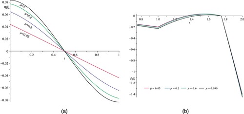\end{aligned}$ (128) The graph of the function $q^{*}$ is clarified in Figure (a) for different values of μ.

Figure 1. (a) The graph of the solution function given by (Equation128(128) $\begin{aligned} q^{*} (t) & = \frac{t^{4 - μ}}{Γ (5 - μ)} - \frac{t^{3 - μ}}{2 Γ (4 - μ)} \\ - \frac{(1 - t)^{4 - μ}}{Γ (5 - μ)} + \frac{(1 - t)^{3 - μ}}{2 Γ (4 - μ)} . \end{aligned}$ (128) ) for different values of μ (b) The graph of the solution function given by (Equation131(131) $\begin{aligned} p (s) & = ϕ (s) = (\frac{3}{4 Γ (6 - μ)} - \frac{1}{4 Γ (4 - μ)} - \frac{1}{6}) s, \\ f o r s \in [\frac{3}{4}, 1], \end{aligned}$ (131) ), (Equation136(136) $\begin{aligned} p (s) & = \frac{3 (s - 1)^{4 - μ}}{2 Γ (5 - μ)} - \frac{3 (s - 1)^{5 - μ}}{4 Γ (6 - μ)} \\ - \frac{(s - 1)^{3 - μ}}{2 Γ (4 - μ)} + \frac{3 (2 - s)^{5 - μ}}{4 Γ (6 - μ)} \\ - \frac{(2 - s)^{3 - μ}}{4 Γ (4 - μ)} - \frac{s^{3}}{6} - (s - 1) [\frac{1}{Γ (5 - μ)} {(\frac{3}{4})}^{4 - μ} \\ - \frac{1}{Γ (6 - μ)} {(\frac{3}{4})}^{5 - μ} - \frac{2}{3 Γ (4 - μ)} {(\frac{3}{4})}^{3 - μ} \\ + \frac{1}{Γ (6 - μ)} {(\frac{1}{4})}^{5 - μ} \\ - \frac{1}{3 Γ (4 - μ)} {(\frac{1}{4})}^{3 - μ}] \\ + \frac{2 (s - 1)}{9} {(\frac{7}{4})}^{3}, s \in [1, \frac{7}{4}] \\ + \frac{2 (s - 1)}{9} {(\frac{7}{4})}^{3}, s \in [1, \frac{7}{4}], \end{aligned}$ (136) ) and (Equation137(137) $\begin{aligned} p (s) & = \frac{1}{2} [\frac{3 Γ (3)}{Γ (5 - μ)} (s - 1)^{4 - μ} - \frac{Γ (4)}{Γ (6 - μ)} (s - 1)^{5 - μ} \\ - \frac{2 Γ (2)}{Γ (4 - μ)} (s - 1)^{3 - μ} + \frac{Γ (4)}{Γ (6 - μ)} (2 - s)^{5 - μ} \\ - \frac{Γ (2)}{Γ (4 - μ)} (2 - s)^{3 - μ}] - \frac{s^{3}}{6} \\ + 2 (s - 2) [\frac{3 Γ (3)}{Γ (5 - μ)} {(\frac{3}{4})}^{4 - μ} - \frac{Γ (4)}{Γ (6 - μ)} \\ \times {(\frac{3}{4})}^{5 - μ} - \frac{2 Γ (2)}{Γ (4 - μ)} {(\frac{3}{4})}^{3 - μ} \\ + \frac{Γ (4)}{Γ (6 - μ)} {(\frac{1}{4})}^{5 - μ} - \frac{Γ (2)}{Γ (4 - μ)} {(\frac{1}{4})}^{3 - μ}] \\ - (s - 2) \frac{4 {(\frac{7}{4})}^{3}}{3}, s \in [\frac{7}{4}, 2] . \end{aligned}$ (137) ) for different values of μ.

Figure 1. (a) The graph of the solution function given by (Equation128(128) q∗(t)=t4−μΓ(5−μ)−t3−μ2Γ(4−μ)−(1−t)4−μΓ(5−μ)+(1−t)3−μ2Γ(4−μ).(128) ) for different values of μ (b) The graph of the solution function given by (Equation131(131) p(s)=ϕ(s)=34Γ(6−μ)−14Γ(4−μ)−16s,for s∈34,1,(131) ), (Equation136(136) p(s)=3(s−1)4−μ2Γ(5−μ)−3(s−1)5−μ4Γ(6−μ)−(s−1)3−μ2Γ(4−μ)+3(2−s)5−μ4Γ(6−μ)−(2−s)3−μ4Γ(4−μ)−s36−(s−1)1Γ(5−μ)344−μ−1Γ(6−μ)345−μ−23Γ(4−μ)343−μ+1Γ(6−μ)145−μ−13Γ(4−μ)143−μ+2(s−1)9743,s∈1,74+2(s−1)9743,s∈1,74,(136) ) and (Equation137(137) p(s)=123Γ(3)Γ(5−μ)(s−1)4−μ−Γ(4)Γ(6−μ)(s−1)5−μ−2Γ(2)Γ(4−μ)(s−1)3−μ+Γ(4)Γ(6−μ)(2−s)5−μ−Γ(2)Γ(4−μ)(2−s)3−μ−s36+2(s−2)3Γ(3)Γ(5−μ)344−μ−Γ(4)Γ(6−μ)×345−μ−2Γ(2)Γ(4−μ)343−μ+Γ(4)Γ(6−μ)145−μ−Γ(2)Γ(4−μ)143−μ−(s−2)47433,s∈74,2.(137) ) for different values of μ.

Example 8.2

Let $r = \frac{1}{4}, a = 1, b = 2,$ and consider the functional (129) $F [p] = \int_{a}^{b} L (s, p (s),_{a}^{R H} D_{b}^{μ, 0} p (s), p (s - r), p^{'} (s - r)) d s,$ (129) where for $s \in [1, 2]$ (130) $\begin{aligned} L (s, p (s),_{b}^{R H} D_{b}^{μ, 0} p (s), p^{'} (s), p (s - r), p^{'} (s - r)) \\ = s p (s) + (6 s^{2} - s^{3} - 11 s + 6)_{a}^{R H} D_{b}^{μ, 0} p (s) - \frac{1}{2} [p^{'} (s)]^{2} \\ + (s - \frac{1}{4}) p (s - r) - \frac{1}{2} {[p^{'} (s - \frac{1}{4})]}^{2} . \end{aligned}$ (130) We find a function p such that $F [p]$ is an extremum and satisfies the boundary conditions: (131) $\begin{aligned} p (s) & = ϕ (s) = (\frac{3}{4 Γ (6 - μ)} - \frac{1}{4 Γ (4 - μ)} - \frac{1}{6}) s, \\ f o r s \in [\frac{3}{4}, 1], \end{aligned}$ (131) and (132) $\begin{aligned} p (\frac{7}{4}) & = 0, p (2) = \frac{3}{Γ (5 - μ)} - \frac{3}{2 Γ (6 - μ)} \\ - \frac{1}{Γ (4 - μ)} - \frac{4}{3} . \end{aligned}$ (132) By applying Theorem 5.1 the function pmust satisfy the following conditions: (133) $2 p^{''} (s) + 2 s =_{1}^{R H} D_{2}^{μ, 1} (6 s^{2} - s^{3} - 11 s + 6),$ (133) for $s \in [1, \frac{7}{4}]$ and (134) $p^{''} (s) + s =_{1}^{R H} D_{2}^{μ, 1} (6 s^{2} - s^{3} - 11 s + 6),$ (134) for $s \in [\frac{7}{4}, 2]$ . Observe that, according to property (2.1) in [Citation1] it yields (135) $\begin{aligned} _{1}^{R H} D_{2}^{μ, 1} (6 s^{2} - s^{3} - 11 s + 6) \\ =_{1}^{R} D_{2}^{μ} (6 s^{2} - s^{3} - 11 s + 6) \\ = \frac{1}{2} [_{1} D_{s}^{μ} (6 s^{2} - s^{3} - 11 s + 6) \\ -_{s} D_{2}^{μ} (6 s^{2} - s^{3} - 11 s + 6)] \\ = \frac{1}{2} [_{1} D_{s}^{μ} (3 (s - 1)^{2} - (s - 1)^{3} - 2 (s - 1))] \\ + \frac{1}{2} [_{s} D_{2}^{μ} ((2 - s)^{3} - (2 - s))] \\ = \frac{3 (s - 1)^{2 - μ}}{Γ (3 - μ)} - \frac{3 (s - 1)^{3 - μ}}{2 Γ (4 - μ)} - \frac{(s - 1)^{1 - μ}}{Γ (2 - μ)} \\ + \frac{3 (2 - s)^{3 - μ}}{2 Γ (4 - μ)} - \frac{(2 - s)^{1 - μ}}{2 Γ (2 - μ)} . \end{aligned}$ (135) Inserting the expression (Equation135(135) $\begin{aligned} _{1}^{R H} D_{2}^{μ, 1} (6 s^{2} - s^{3} - 11 s + 6) \\ =_{1}^{R} D_{2}^{μ} (6 s^{2} - s^{3} - 11 s + 6) \\ = \frac{1}{2} [_{1} D_{s}^{μ} (6 s^{2} - s^{3} - 11 s + 6) \\ -_{s} D_{2}^{μ} (6 s^{2} - s^{3} - 11 s + 6)] \\ = \frac{1}{2} [_{1} D_{s}^{μ} (3 (s - 1)^{2} - (s - 1)^{3} - 2 (s - 1))] \\ + \frac{1}{2} [_{s} D_{2}^{μ} ((2 - s)^{3} - (2 - s))] \\ = \frac{3 (s - 1)^{2 - μ}}{Γ (3 - μ)} - \frac{3 (s - 1)^{3 - μ}}{2 Γ (4 - μ)} - \frac{(s - 1)^{1 - μ}}{Γ (2 - μ)} \\ + \frac{3 (2 - s)^{3 - μ}}{2 Γ (4 - μ)} - \frac{(2 - s)^{1 - μ}}{2 Γ (2 - μ)} . \end{aligned}$ (135) ) into (Equation133(133) $2 p^{''} (s) + 2 s =_{1}^{R H} D_{2}^{μ, 1} (6 s^{2} - s^{3} - 11 s + 6),$ (133) ) and (Equation134(134) $p^{''} (s) + s =_{1}^{R H} D_{2}^{μ, 1} (6 s^{2} - s^{3} - 11 s + 6),$ (134) ) and taking into account the boundary conditions (Equation131(131) $\begin{aligned} p (s) & = ϕ (s) = (\frac{3}{4 Γ (6 - μ)} - \frac{1}{4 Γ (4 - μ)} - \frac{1}{6}) s, \\ f o r s \in [\frac{3}{4}, 1], \end{aligned}$ (131) ) and (Equation122(122) $\frac{d^{2}}{d^{2}} q^{*} (t) +_{0}^{R H} D_{1}^{μ, 1} (t^{2} - t) = 0, f o r a n y t \in [0, 1],$ (122) ), we get after some manipulations (136) $\begin{aligned} p (s) & = \frac{3 (s - 1)^{4 - μ}}{2 Γ (5 - μ)} - \frac{3 (s - 1)^{5 - μ}}{4 Γ (6 - μ)} \\ - \frac{(s - 1)^{3 - μ}}{2 Γ (4 - μ)} + \frac{3 (2 - s)^{5 - μ}}{4 Γ (6 - μ)} \\ - \frac{(2 - s)^{3 - μ}}{4 Γ (4 - μ)} - \frac{s^{3}}{6} - (s - 1) [\frac{1}{Γ (5 - μ)} {(\frac{3}{4})}^{4 - μ} \\ - \frac{1}{Γ (6 - μ)} {(\frac{3}{4})}^{5 - μ} - \frac{2}{3 Γ (4 - μ)} {(\frac{3}{4})}^{3 - μ} \\ + \frac{1}{Γ (6 - μ)} {(\frac{1}{4})}^{5 - μ} \\ - \frac{1}{3 Γ (4 - μ)} {(\frac{1}{4})}^{3 - μ}] \\ + \frac{2 (s - 1)}{9} {(\frac{7}{4})}^{3}, s \in [1, \frac{7}{4}] \\ + \frac{2 (s - 1)}{9} {(\frac{7}{4})}^{3}, s \in [1, \frac{7}{4}], \end{aligned}$ (136) and (137) $\begin{aligned} p (s) & = \frac{1}{2} [\frac{3 Γ (3)}{Γ (5 - μ)} (s - 1)^{4 - μ} - \frac{Γ (4)}{Γ (6 - μ)} (s - 1)^{5 - μ} \\ - \frac{2 Γ (2)}{Γ (4 - μ)} (s - 1)^{3 - μ} + \frac{Γ (4)}{Γ (6 - μ)} (2 - s)^{5 - μ} \\ - \frac{Γ (2)}{Γ (4 - μ)} (2 - s)^{3 - μ}] - \frac{s^{3}}{6} \\ + 2 (s - 2) [\frac{3 Γ (3)}{Γ (5 - μ)} {(\frac{3}{4})}^{4 - μ} - \frac{Γ (4)}{Γ (6 - μ)} \\ \times {(\frac{3}{4})}^{5 - μ} - \frac{2 Γ (2)}{Γ (4 - μ)} {(\frac{3}{4})}^{3 - μ} \\ + \frac{Γ (4)}{Γ (6 - μ)} {(\frac{1}{4})}^{5 - μ} - \frac{Γ (2)}{Γ (4 - μ)} {(\frac{1}{4})}^{3 - μ}] \\ - (s - 2) \frac{4 {(\frac{7}{4})}^{3}}{3}, s \in [\frac{7}{4}, 2] . \end{aligned}$ (137) The graph of the function p is clarified in Figure (b) for different values of μ.

Remark 8.1

According to Remark 2.2, if $β = 0$ , then $_{a}^{R H} D_{b}^{μ, β} q (t) =_{a}^{R C} D_{b}^{μ} q (t); t \in [a, b]$ , and hence, when $μ = 1$ , we get $_{a}^{R H} D_{b}^{μ, β} q (t) = d q / d; t \in [a, b] .$ So, the figures (a) and (b) emphasize that when $μ$ approach to the value one, the solution function curve approaches to the solution function curve if the Riesz–Hilfer derivative is replaced by the first drivative.

Example 8.3

Fractional Lagrangian for RLC.

In this example we consider a simple loop current that is described by a fractional Lagrangian. We assume that this single loop circuit involves a capacitor C, a resistor R and an inductor χ. The fractional Lagrangian for this loop take the form (138) $L = \frac{χ}{2} {[\frac{d q}{d t}]}^{2} - \frac{1}{2 c} q^{2} (t) + \frac{i γ R}{2}_{b}^{R H} D_{b}^{μ, β} q (t),$ (138) where, q is the charge. According to Theorem 3.1, Euler–Lagrange equation corresponding to (138) is (139) $\frac{q}{c} + χ \frac{d^{2} q}{d^{2}} +_{b}^{R H} D_{b}^{μ, β} (\frac{i γ R}{2}) (t) = 0.$ (139)

Example 8.4

Let $r \in (0, b - a),$ $h : [a, b] \to R$ be such that the function $z (t) =_{a}^{R H} D_{b}^{μ, β} h (t)$ is continuously differentiable. Consider the functional (140) $J [q] = \int_{a}^{b} (\frac{1}{2} q^{2} (t) + h (t)_{a}^{R H} D_{b}^{μ, 1} q (t) + \frac{1}{2} [q^{'} (t - r)]^{2}) d t,$ (140) with the boundary conditions (141) $q (t) = ϕ (t), t \in [a - r, a] a n d q (b) = q^{b} .$ (141) According to Theorem 5.1, the functional J has an extremum at a function q if q satisfies: (142) $q (t) -_{a}^{R C} D_{b}^{μ} h (t) - q^{''} (t - r) = 0, f o r t \in [a, b - r],$ (142) and (143) $q (t) -_{a}^{R C} D_{b}^{μ} h (t) = 0, f o r t \in [b - r, b] .$ (143)

Remark 8.2

Like in many papers, see for example [Citation21], the numerical methods are more suitable to find the solutions of FVP.

9. Results and discussion

As mentioned earlier, variational problems and fractional calculus have many applications in different branches in engineering and mathematics, moreover, the Riesz–Hilfer fractional derivative (RHFD) is a generalization for the Riesz–Riemann–Liouville and the Riesz–Caputo derivative. The results that we obtained are to find Euler–Lagrange equations for various of fractional variational problems with the Lagrangian function containing (RHFD), and hence our results generalize many recent papers in the literature, for example, [Citation22–25, Citation36]. On other hand, our technique allows to generalize some works, such as the obtained results in [Citation26] to the case when the functional involving (RHFD). As we mentioned in Corollary 2.1, relations (Equation20(20) $\begin{aligned} \int_{a}^{b} h (t)_{a}^{R} D_{b}^{μ} η (t) d t \\ = \int_{a}^{b} h (t)_{a}^{R H} D_{b}^{μ, 1} η (t) d t \\ = - \int_{a}^{b} η (t)_{a}^{R H} D_{b}^{μ, 0} h (t) d t + \frac{1}{2} h (t)_{a} I_{t}^{1 - μ} η (t) |_{a}^{b} \\ + \frac{1}{2} h (t)_{t} I_{b}^{1 - μ} η (t) |_{a}^{b} \\ = - \int_{a}^{b} η (t)_{a}^{R C} D_{b}^{μ} h (t) d t + h (t)_{a}^{R} I_{b}^{1 - μ} η (t) |_{a}^{b} . \end{aligned}$ (20) ) and (Equation21(21) $\begin{aligned} \int_{a}^{r} h (t)_{a}^{R H} D_{b}^{μ, β} η (t) d t \\ = - \int_{a}^{r} η (t)_{a}^{R H} D_{b}^{μ, 1 - β} h (t) d t \\ + \frac{1}{2} [\int_{a}^{r} η (t) (_{t} D_{r}^{μ, 1 - β} -_{t} D_{b}^{μ, 1 - β}) h (t)) d t \\ +_{t} I_{r}^{q} h (t) ._{a} I_{t}^{β (1 - μ)} η (t) |_{a}^{r} \\ - \int_{r}^{b} η (t) (_{a} D_{t}^{μ, 1 - β} -_{r} D_{t}^{μ, 1 - β}) h (t) d t \\ + a I_{t}^{q} h (t) ._{t} I_{b}^{β (1 - μ)} η (t) |_{a}^{b} \\ - r I_{t}^{q} h (t) ._{t} I_{b}^{β (1 - μ)} η (t) |_{r}^{b}] . \end{aligned}$ (21) ) in [Citation22] are particular cases of Lemma 2.1, and if $β = 0$ and i = 1 in Theorem 3.1, then we obtain Theorem 3.1, in [Citation22]. Moreover, If we put $β = 0$ in both Theorems 3.2 and 6.1, we obtain Theorems 4.1 and 7.1, respectively, in [Citation24].

10. Conclusion

Euler–Lagrange equations for different kind of fractional variational problems with the Lagrangian function containing the Riesz–Hilfer fractional derivative are obtained. Since the Riesz–Hilfer fractional derivative is a generalization for the Riesz–Riemann–Liouville and the Riesz–Caputo derivative, then our results generalize many recent works in which the Lagrangian function involving the Riesz–Riemann–Liouville or the Riesz–Caputo derivative. Fractional variational problem in the presence of delay derivatives is considered. Moreover, a version for Noether theorem in the Riesz–Hilfer sense is established. Necessary conditions for a pair function-time to be an optimal solution to the problem are investigated. Examples are given to illustrate the applicability of the obtained results. Furthermore, our obtained results generalize some existing results such as Theorem 1 in [Citation22] and Theorems 3 and 6 in [Citation24]. Also, the technique used in the present paper enable to extend the results in [Citation26, Citation28, Citation31] when the treated problems in these works involving Riesz–Hilfer fractional derivative. Moreover, this work, may be, encourages to study partial differential equations containing Riesz–Hilfer fractional derivative.

Acknowledgments

The authors acknowledge the Deanship of Scientific Research at King Faisal University for financial support under the Research Group Support Track. (Grant No. 1811003).

Disclosure statement

No potential conflict of interest was reported by the author(s).

Additional information

Funding

The authors acknowledge the Deanship of Scientific Research at King Faisal University for financial support under the Research Group Support Track [grant number 1811003].

References

Kilbas AA, Srivastava HM, Trujillo JJ, Theory and applications of fractional differential equations, Amsterdam: Elsevier Science Publishers BV; 2006. (North holland mathematics studies; vol. 204).
Google Scholar
Miller KS, Ross B. An introduction to the fractional calculus and fractional differential equations. New York: Wiley; 1993.
Google Scholar
Podlubny I. Fractional differential equations. San Diego (CA): Academic Press; 1999.
Google Scholar
Smako SG, Kilbas AA, Marichev OI. Fractional integral and derivativies-theory and applications. Longhorne (PA): Gordan and Breach; 1993.
Google Scholar
Ghomanjani F. A new approach for solving fractional differential algebric equations. J Taibah Univ Sci. 2017;11:1158–1164.
Web of Science ®Google Scholar
Ibrahim AG. Differential equations and inclusions of fractional order with impulse effect in Banach spaces. Bull Malays Math Sci Soc. 2020;43(1):69–109.
Web of Science ®Google Scholar
Moghaddam BP, Mostaghim ZS. A numercial method based on finite difference for solving fractional delay differential equations. J Taibah Univ Sci. 2013;7:120-127.
Google Scholar
Lukashchuk SY. Approximate conservation laws for fractional differential equations. Commun Nonlinear Sci Numer Simul. 2019;68:147–159.
Web of Science ®Google Scholar
Wang JR, Ibrahim AG, O'Regan D, et al. A general class of noninstantaneous impulsive fractional differential inclusions in Banach spaces. Adv Differ Equ. 2017;2017(1):1–28. DOI:10.1186/s13662-017-1342-8
Google Scholar
Wang JR, Ibrahim AG, O'Regan D. Hilfer- type fractional differential switched inclusions with noninstantaneous impulsive and nonlocal conditions. Nonlinear Anal Model Control. 2018;23(6):921–941.
Web of Science ®Google Scholar
Wang JR, Ibrahim AG, O'Regan D. Controllability of noninstantaneous impulsive semilinear functional differential inclusions without compactness. Indag Math New Ser. 2018;29:1362–1392.
Web of Science ®Google Scholar
Wang JR, Ibrahim AG, O'Regan D. Controllability of fractional evolutions inclusions with noninstantaneous impulsive. Int J Nonlinear Sci Numer Simul. 2018;19(3-4):321–334.
Web of Science ®Google Scholar
Wang JR, Ibrahim AG, O'Regan D. Global attracting solutions to Hilfer fractional differential inclusions of Sobolev type with noninstantaneous impulses and nonlocal conditions. Nonlinear Anal Model Control. 2019;24(5):775–803.
Web of Science ®Google Scholar
Wang JR, Ibrahim AG, O'Regan D. Nonemptyness and compactness of the solution set for fractional evolution inclusions with non-instantaneous impulses. Electron J Differ Equ. 2019;37:1–17.
Google Scholar
Bliss GA. Lectures on the calculus of variations. University of Chicago Press; 1963.
Google Scholar
Gelfand IM, Fomin SV. Calculus of variations. Prenticc-Hail; 1963.
Google Scholar
Hestenes MR. Calculus of variations and optimal control theory. John Wiley & Sons; 1966.
Google Scholar
Weinstock R. Calculus of variations with applications to physics and engineering. New-York: Dover publications, Inc.; 1974.
Google Scholar
Riewe F. Nonconservative Lagrangian and Hamiltonian mechanics. Phys Rev E. 1966;53(2):1890–1899.
Google Scholar
Riewe F. Mechanics with fractional derivatives. Phys Rev E. 1997;55(3):3581–3592.
Web of Science ®Google Scholar
Agrawal OP. Formulation of Euler–Lagrange equations for fractional variational problems. J Math Anal Appl. 2002;272:368–379.
Web of Science ®Google Scholar
Agrawal OP. Fractional variational calculus in terms of Riesz fractional derivatives. J Phys A Math Theor. 2007;40:6287–6303.
Web of Science ®Google Scholar
Almeida R, Torres DFM. Necessary and sufficient conditions for the fractional calculus of variations with Caputo derivatives. Commun Nonlinear Sci Numer Simul. 2011;16(3):1490–1500.
Web of Science ®Google Scholar
Almeida R. Fractional variational problems with the Riesz–Caputo derivative. Appl Math Lett. 2012;25:142–148.
Web of Science ®Google Scholar
Odzijewicz T, Malinowska AB, Torres DFM. Fractional variational calculus with classical and combined Caputo derivatives. Nonlinear Anal. 2012;75:1507–1515.
Web of Science ®Google Scholar
Sayev K, Rostami MR, Attari HS. A new study on delay fractional variation problems. Int J Comput Math. 2018;95(6-7):1170–1194.
Web of Science ®Google Scholar
Tavares D, Almeida R, Torres DFM. Optimality conditions for fractional variational problems with dependence on a combined Caputo derivative of.variable order. Optimization. 2015;64(6):1381–1391.
Web of Science ®Google Scholar
Almeida R, Morgado ML. The Euler–Lagrange and Legendre equations for functionals involving distributed-order fractional derivatives. Appl Math Comput. 2018;331:394–403.
Web of Science ®Google Scholar
Agrawal OP. Generalized variational problems and Euler–Lagrange equations. Comput Math Appl. 2010;59:1852–1864.
Web of Science ®Google Scholar
Almeida R, Pooseh S, Torres DFM. Computational methods in the fractional calculus of variations. London: Imp. Coll. Press; 2015.
Google Scholar
Askari H, Ansari A. Fractional calculus of variations with a generalized fractional derivative. Fract Differ Calc. 2016;6:57–72.
Google Scholar
Atanacković TM, Pilipović S. Variational problems with fractional derivatives: Euler–Lagrange equations. J Phys A Math Theor. 2011;41(9):195–201.
Google Scholar
Baleanu D. About fractional quantization and fractional variational principles. Commun Nonlinear Sci Numer Simul. 2009;14(6):2520–2523.
Web of Science ®Google Scholar
Baleanu D, Trujillo JI. A new method of finding the fractional Euler–Lagrange and Hamilton equations within Caputo fractional derivatives. Common Nonlinear Sci Numer Simul. 2010;15(5):1111–1115.
Web of Science ®Google Scholar
Herzallah MAE, Baleanu D. Fractional-order Euler–Lagrange equations and formulation of Hamiltonian equations. Nonlinear Dyn. 2009;58(1-2):385–391.
Web of Science ®Google Scholar
Jarad F, Abdeljawad T, Baleanu D. Fractional variational principles with delay within Caputo derivatives. Rep Math Phys. 2010;65(1):17–28.
Web of Science ®Google Scholar
Malinowska AB, Torres DFM. Generalized natural boundary conditions for fractional variational problems in terms of the Caputo derivative. Comput Math Appl. 2010;59(9):3110–3116.
Web of Science ®Google Scholar
Malinowska AB, Torres DFM. Fractional variational calculus in terms of a combined Caputo derivative. In: Proceedings IFAC Workshop on Fractional Derivative and Applications IFAC FDA2010. Badajoz, Spain: University of Extremadura; 2010. p. 18–20.
Google Scholar
Tavares D, Almeida R, Torres DFM. Constrained fractional variational problems of variable order. IEEE/CAA J Autom Sin. 2017;1(4):65–73.
Google Scholar
Tavares D, Almeida R, Torres DFM. Combined fractional variational problems of variable order and some computational aspects. J Comput Appl Math. 2018;339:374–388.
Web of Science ®Google Scholar
Hilfer R. Applications of fractional calculus in physics. Singapore: World Scientific; 1999.
Google Scholar
Agrawal OP, Muslih SI, Baleanu D. Generalized variational calculus in terms of multiparamaters fractional derivatives. Commun Nonlinear Sci Numer Simul. 2010;16:4756–4767.
Web of Science ®Google Scholar
Ali A, Seadawy AR, Lu D. Computational methods and traveling wave solutions for the fourth-order nonlinear Ablowitz-Kaup-Newell-Segur water wave dynamical equation via two methods and its applications. Open Phys. 2018;16:219–226.
Web of Science ®Google Scholar
Iqbal M, Seadawy AR, Lu D. Construction of solitary wave solutions to the nonlinear modified Kortewege-de Vries dynamical equation in unmagnetized plasma via mathematical methods. Mod Phys Lett A. 2018;33(32):1850183.
Web of Science ®Google Scholar
Iqbal M, Seadawy AR, Lu D. Dispersive solitary wave solutions of nonlinear further modified Korteweg–de Vries dynamical equation in an unmagnetized dusty plasma. Mod Phys Lett A. 2018;33(37):1850217.
Web of Science ®Google Scholar
Iqbal M, Seadawy AR, Lu D. Construction of bright–dark solutions and ion-acoustic solitary wave solutions of dynamical system of nonlinear wave propagation. Mod Phys Lett A. 2019;34(37):1950309.
Web of Science ®Google Scholar
Iqbal M, Seadawy AR, Lu D, et al. Construction of a weakly nonlinear dispersion solitary wave solution for the Zakharov–Kuznetsov-modified equal width dynamical equation. Indian J Phys. 2019;21:1–10.
Google Scholar
Iqbal M, Seadawy AR, Khalil OH, et al. Propagation of long internal waves in density stratified ocean for the (2+1)-dimensional nonlinear Nizhnik-Novikov-Vesselov dynamical equation. Res Phys. 2020;16:102838.
Google Scholar
Iqbal M, Seadawy AR, Lu D. Applications of nonlinear longitudinal wave equation in a magneto-electro-elastic circular rod and new solitary wave solutions. Mod Phys Lett B. 2019;33(18):1950210.
Web of Science ®Google Scholar
Lu D, Seadawy AA, Iqbal M. Mathematical methods via construction of traveling and solitary wave solutions of three coupled system of nonlinear partial differential equations and their applications. Res Phys. 2018;11:1161–1171.
Google Scholar
Nasreen N, Seadawy AR, Lu D, et al. Dispersive solitary wave and soliton solutions of the generalized third order nonlinear Schrodinger dynamical equation by modified analytical method. Res Phys. 2019;15:102641.
Google Scholar
Seadaway AR, Lu D, Yue C. Travelling wave solutions of the generalized nonlinear fifth-order KDV water wave equations and its stability. J Taibah Univ Sci. 2017;11:623–633.
Web of Science ®Google Scholar
Seadawy AR, Iqbal M, Lu D. Nonlinear wave solutions of the kudryashov–Sinelshchikov dynamical equation in mixtures liquid-gas bubbles under the consideration of heat transfer and viscosity. J Taibah Univ Sci. 2019;13:1060–1072.
Web of Science ®Google Scholar
Seadawy AR, Iqbal M, Lu D. Propagation of kink and anti-kink wave solutions for the nonlinear damped modified Korteweg–de Vries equation arising in ion-acoustic wave in an unmagnetized collisional dusty plasma. Phys A. 2020;544:123560.
Web of Science ®Google Scholar
Seadawy AR, Iqbal M, Lu D. Construction of soliton solutions of the modify unstable nonlinear Schrodinger dynamical equation in fiber optics. Indian J Phys. 2019:1–10.
Web of Science ®Google Scholar
Seadawy AR, Lu D, Iqbal M. Application of mathematical methods on the system of dynamical equations for the ion sound and Langmuir waves. Pramana J Phys. 2019;93(1):10.
Web of Science ®Google Scholar
Seadawy AR, Iqbal M, Lu D. Applications of propagation of long-wave with dissipation and dispersion in nonlinear media via solitary wave solutions of generalized Kadomtsev–Petviashvili modified equal width dynamical equation. Comput Math Appl. 2019;78:3620–3632.
Web of Science ®Google Scholar

Euler–Lagrange equations for variational problems involving the Riesz–Hilfer fractional derivative

Abstract

1. Introduction

2. Preliminaries and notations

[Citation1]

[Citation41]

[Citation41]

3. Euler–Lagrange equation for a simple fractional variational problem involving the Riesz–Hilfer derivative

4. Isoperimetric problem

5. Fractional variational problem with delay

6. Optimal time problem

7. The Noether theorem in the sense of Riesz–Hilfer

8. Applications

9. Results and discussion

10. Conclusion

Acknowledgments

Disclosure statement

References

Information for

Open access

Opportunities

Help and information

Euler–Lagrange equations for variational problems involving the Riesz–Hilfer fractional derivative

Abstract

1. Introduction

2. Preliminaries and notations

[Citation1]

[Citation41]

[Citation41]

3. Euler–Lagrange equation for a simple fractional variational problem involving the Riesz–Hilfer derivative

4. Isoperimetric problem

5. Fractional variational problem with delay

6. Optimal time problem

7. The Noether theorem in the sense of Riesz–Hilfer

8. Applications

9. Results and discussion

10. Conclusion

Acknowledgments

Disclosure statement

Additional information

Funding

References

Related research

To cite this article:

Download citation

Your download is now in progress and you may close this window

Login or register to access this feature

Information for

Open access

Opportunities

Help and information

Keep up to date