
 ?Mathematical formulae have been encoded as MathML and are displayed in this HTML version using MathJax in order to improve their display. Uncheck the box to turn MathJax off. This feature requires Javascript. Click on a formula to zoom.
Abstract
A numerical treatment to a system of Caputo fractional order differential- algebraic equations (SFDAEs) is presented throughout this article. The suggested method based upon the shifted Chebyshev pesedu- spectral method (SCPSM). The shifted Chebyshev polynomials (SCPs) are handled to reduce the SFDAEs into the solution of linear/ nonlinear systems of algebraic equations. By using some tested applications, the effectiveness and the accuracy of the suggested approach are demonstrated graphically. Also numerical comparisons between the proposed technique with other numerical methods in the existing literature are held. The numerical results show that the proposed technique is computationally efficient, accurate and easy to implement.
1. Introduction
Nowadays, the fractional differential equations (FDEs) have gained increased appearances in varied problems in various fields of physics, chemistry, biology, applied science and engineering, this is due to their accuracy in modelling these problems [Citation1–8]. Consequently, the development of analytical and numerical algorithms for FDEs is an interested topic for many researches [Citation9–16].
Many physical phenomena's are obviously designated by a system of differential-algebraic equations (SDAEs). These types of systems follow in the displaying of the mechanical systems subject to constraints, power systems, electrical networks, optimal control, chemical process and in other numerous applications [Citation17]. SFDAEs have currently confirmed to be a suitable devise in the displaying of the numerous engineering and physical problems such as non-integer order optimal controller design, electrochemical processes, complex biochemical [Citation18].
The approximate and numerical solutions of these types of systems have been a focus of several researchers especially the nonlinear systems, because most of these systems don't have exact solutions. Numerical methods to solve SDAEs have been given such as, the numerical algorithms for computing the matrix Green's operator [Citation19], implicit Runge–Kutta method [Citation20], Padé approximation method [Citation21,Citation22], homotopy perturbation method [Citation23], Adomain decomposition method [Citation24] and variation iteration method (VIM) [Citation25].
While methods like, the homotopy analysis method (HAM) [Citation26], the Adomian decomposition method (ADM) [Citation27], the variational iteration method [Citation27], fractional differential transform method [Citation28], the generalized triangular function operational matrices [Citation29], the Bezier curves method [Citation30], and Gegenbauer tau method [Citation31] have been successfully applied for SFDAEs.
In this paper, we apply the SCPSM to solve the following SFDAEs [Citation31]:
(1)
(1) With the initial conditions:
(2)
(2) where
is the Caputo fractional derivative of order
. When
, the SFDAEs is reduced to the classical SDAEs. The proposed technique is one of the known spectral methods, which have been widely used in many fields. These methods are characterized by their speed of convergence and the high level of accuracy.
For FDEs, the spectral collocation method (also called pseudo-spectral method) is more applicable and commonly applied to numerically solve different types of the fractional differential equations [Citation15,Citation32]. In collocation technique, expansion coefficients are determined by constructing the approximate solution to satisfy the differential equation at some applicably selected points from the domain identified as collocation points. Recently, various types of orthogonal polynomials and collocation points are used in spectral collocation approximations [Citation15,Citation32].
CPs have many useful properties. These polynomials present, among others, very good properties in the approximation of functions. This encourages many researchers for using these polynomials for solving different types of differential equations and FDEs [Citation32–35].
The proposed technique used the properties of Chebyshev polynomials (CPs) to reduce the SFDAEs into a system of algebraic equation which is greatly simplifying the problem. To the best of our knowledge, the numerical treatment of SFDAEs has not been established by using SCPSM yet.
To check the accuracy of the suggested method, five numerical applications including comparisons between our obtained results with those achieved by using other existing methods are presented. This article is prescribed as follows: The basic definition of the Caputo fractional derivative and the main properties of the CPs are summarized in Section 2. In Section 3, the necessary theorems of the upper bound of errors and the convergence analysis of the fractional derivatives of the SCPs are explained. Section 4 contains the procedures for the implementation of the suggested method to nonlinear FDAEs. Some applications are discussed in Section 5. Finally, a brief conclusion finishes the paper in Section 6.
2. Preliminaries and notations
2.1. Caputo fractional derivatives
Definition 2.1:
A real function is assumed to be in the space
if there exists a real number
such that
where
and is assumed to be in space
if and only if
Definition 2.2
The fractional derivative of
in the Caputo sense is defined as
(3)
(3) For
Caputo derivatives have the following properties:
(4)
(4)
(5)
(5) where
is the ceiling function and
For
the Caputo fractional derivative agrees with the integer order derivative. More details in [Citation12,Citation13].
2.2. Main properties of the CPs
The CPs, of degree
are determined by the following recurrence relation [Citation32–34]
The analytic form of
is defined by
(6)
(6) where
is the integer part of
.
The SCPs of degree n defined in the interval
, constructed by offering the change of variable
and defined by
(7)
(7) The square integrable function
in
can be approximated using the first
terms of the SCPs as
(8)
(8) Where the coefficients
are given by
(9)
(9)
3. The approximation of the fractional derivatives of the SCPs and its convergence analysis
The approximate formulation of the non-integer derivatives, the truncating error and the convergence analysis of the SCPs are considered in the following theorems.
Theorem 2.1:
(Chebyshev truncation theorem) [Citation32]
The error in approximating by the sum of its
-terms is bounded by the sum of the absolute values of all neglected coefficient. If
(10)
(10) then
(11)
(11)
Theorem 2 .2:
Let be approximated by SCPs as in (8) and suppose that
, then
(12)
(12) Where
is given by
(13)
(13) For Proof, see [Citation32].
Theorem 2.3
The Caputo fractional derivative of order for the SCPs can be expressed in terms of the SCPs themselves as in the following form
(14)
(14) where
(15)
(15) Theorem 3.4 [Citation32,Citation35]
The error in approximating
is bounded by:
(16)
(16)
4. Solution to the SFDAEs
In this section we will explain the main steps of the procedure of applying the SCPSM for solving the following SFDAEs:
(17)
(17) Subject to the initial conditions
(18)
(18) Step 1: Approximate
by using the SCPs as:
(19)
(19) Step 2: Use Eq. (12) to approximate the Caputo fractional derivatives, then the SFDAEs (17) is reduced to
(20)
(20) Step 3: Approximate the initial conditions (18) by using SCPs:
(21)
(21) Step 4: Collocate Eq. (20) at the
points. For a suitable collocation points, use the of the SCPs roots,
.
Step 5: The obtained equations of the previous step 4 with Eq. (21) represent a system of linear/nonlinear algebraic equations which contain of unknowns;
,
Step 6: Solve the algebraic system by using the Newton iteration method to obtain the unknowns.
Step 7: The approximated solutions will be
5. Numerical applications
In this section five numerical applications of SFDAEs are solved by the proposed technique; the applications include variable and constant coefficient linear\ nonlinear SFDAEs
Application 5.1:
Consider the following variable coefficient linear SFDAE [Citation27–29]
(22)
(22) With the initial conditions
(23)
(23) For the special case at
system (22) has exact solution:
(24)
(24) By implementing the proposed technique using
,
and
to Eq. (22), we obtain
(25)
(25) And the approximated equations for the initial conditions will be
(26)
(26) The equations obtained by collocating system (25) at the first five roots of the SCPs
with Eqs. (26) represent a system of linear algebraic equations which contains twelve equations for twelve unknowns;
and
. These unknowns are obtained by using Newton iteration method.
For . The estimated solutions are
Figure (a,b) shows the performance of the approximate solutions;
and
respectively, of the Application 5.1 at
for different values of
(
= 0.75,
= 0.85,
= 0.95,
= 1) with the exact solutions at
. it is easy to see that the obtained solutions are continuously depended on the fractional derivative and the estimated solutions are in good agreement with the exact solution at
The Absolute errors between the exact solution and the approximate solution of Application 5.1 at different values of
(
) with their CPU time are tabulated in Table . Executing time of this problem is measured using Mathematica 10 software on CPU Intel(R) Core(TM) i3, it's apparent that the solution doesn't require much CPU time. It is remarkable that the proposed technique is very effective even with using few terms of SCPs and the overall errors can be made smaller by adding more terms of SCPs.
Figure 1. The behaviours of and
of Application 5.1 for different values of
with the exact solutions at
. (a)
, (b)
.
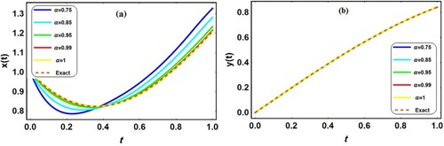
Table 1. Absolute error of  of Application 5.1 for different values of .
In Table the approximate numerical solutions for for
are compared with the solutions given by VIM [Citation27], HAM [Citation28] and TF [Citation29]. These numerical results demonstrate the harmony between our method and the other numerical methods used in the comparisons.
Table 2. Approximate solution of obtained by our proposed method with the results in [Citation27–29].
Application 5.2:
Consider the following nonlinear SFADE [Citation27–29]
(27)
(27) With
and initial conditions
(28)
(28) For the special case when
the exact solution is
.
By employing the proposed technique using ,
and
We obtain a system of nonlinear algebraic equations which contains eighteen equations for eighteen unknowns; ,
. These unknowns are obtained by using Newton iteration method.
For . The estimated solutions will be
The numerical solutions of Application 5.2 are shown graphically through Figure and tabulated in Table (a–c) and Table (4a and 4b). From Figure , it is easy to conclude that the obtained solutions are continuously depend on the fractional derivative and the estimated solutions are in good agreement with the exact solution at
. Table (a–c) show the effectiveness of the suggested technique even with using few terms of SCPs and the accuracy of the method is increased by adding more terms of the SCPs. Also the solutions do not need much CPU time to produce very accurate numerical solutions.
Table 3. (a) Absolut errors of of Application 5.2 for different values of .
Table (a,b) demonstrate the accuracy of the proposed technique when compared with the numerical methods in [Citation27–29].
Figure 2. The behaviours of of Application 5.2 for different values of
with the exact solutions at
= 1,
; (a)
, (b)
, (c)
.
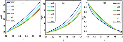
Table 4. (a) The approximate solution of of Application 5.2 with comparisons by [Citation27–29].
Table 5. (a) The absolute error of of Application 5.3 for different values of .
Table 6. (a) The absolute error of of Application 5.4 for different values of .
Table 7. (a) Numerical comparison between the approximate solutions of of Application 5.5 with SGOM [Citation31] at .
Application 5.3:
Consider the following variable coefficient nonlinear SFDAEs [Citation29]
(29)
(29) where
and initial conditions:
(30)
(30) At
The exact solution is:
.
By applying our proposed technique using ,
,
and
to the fractional system (5–8), we obtain a system of linear algebraic equations with unknowns;
,
. These unknowns are attained by using Newton iteration method. For
, the estimated solutions will be
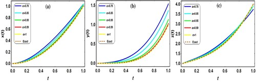
The numerical solutions of Application 5.3 are shown graphically through Figure and the absolute errors between our approximate solutions and the exact solutions for different values of m with their CPU time are given in Table (a–c)
Application 5.4:
Consider the following nonlinear SFDAEs [Citation26]
(31)
(31) with the initial conditions
(32)
(32) At
System (31) has exact solution:
. By using our proposed technique using
and
to the fractional system (5–6), we obtain a system of linear algebraic equations with unknowns;
,
. These unknowns are gained by using Newton iteration method.
Figure 3. The behaviour of of Application 5.3 for different values of
with exact solutions
; (a)
, (b)
, (c)
.

For , the estimated solutions are
The numerical solutions of Application 5.4 are shown graphically through Figure and the absolute errors for different values of
are tabulated in Table (a–c).
Figure 4. The behaviours of Application 5.4 for different values of
with exact solutions at
; (a)
, (b)
, (c)
.
Application 5.5:
Consider the following SFDAEs [Citation31]
(33)
(33) with the initial conditions
(34)
(34) The exact solution of this problem is
(35)
(35) By using our proposed technique using
and
to the fractional system (33), we obtain a system of linear algebraic equations with unknowns;
,
. These unknowns are obtained by solving the algebraic system. Then the estimated solutions are
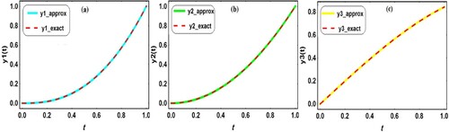
The numerical results of Application 5.5 are graphically illustrated in Figure . A numerical comparison between our attained solutions with the results in [Citation31] is tabulated in Table (a–c). The numerical results demonstrate the effectiveness and the accuracy of the proposed technique even by using a few terms of SCPs, and our obtained results are quite similar to the results given by SGOM [Citation31].
5. Conclusion
Through this paper, The SCPSM method has been extended to solve the linear and nonlinear SFDAEs. The numerical results of some tested applications were a good evidence for the applicability and efficiency of the suggested method. A specific advantage of the suggested implementation is that it transfers the fractional differential equations into a system of algebraic equations which is easier to solve. Also, satisfactory results are obtained by using a few terms of the SCPs, and the efficiency of the anticipated method is increased by using more terms of SCPs. The obtained solutions are continuously depended on the fractional derivative and this note confirms the physical meaning of the behaviour of the solution for the proposed real problems. Also the solutions do not require much CPU time.
Figure 5. The behaviours of the approximate and exact solutions of Application 5.5. (a) (b)
(c)
.
Acknowledgement
The author is very grateful to the referees for carefully reading the paper and for their comments and suggestions which have improved the paper.
Disclosure statement
No potential conflict of interest was reported by the author(s).
References
- Butzer PL, Westphal U. An introduction to fractional calculus. Ch. 1. In: Hilfer R, editor. Applications of fractional calculus in physics. Singapore: World Scientific; 2000. p. 87–130.
- Debnath L. Fractional integral and fractional differential equations in fluid mechanics. Fract. Calc. Appl. Anal. 2003;6:119–155.
- Samko SG, Kilbas AA, Marichev OI. Fractional integrals and derivatives: Theory and applications. Amsterdam: Gordan and Breach. 1993.
- Ullah R, Ellahi R, Sait SM, et al. On the fractional-order model of HIV-1 infection of CD4+ T-cells under the influence of antiviral drug treatment. J Taibah Univ Sci. 2020;14(1):50–59. doi: 10.1080/16583655.2019.1700676
- Coronel-Escamilla A, Torres F, Gómez-Aguilar JF, et al. On the trajectory tracking control for an SCARA robot manipulator in a fractional model driven by induction motors with PSO tuning. Multibody Syst Dyn. 2018;43(3):257–277. doi: 10.1007/s11044-017-9586-3
- Gómez-Aguilar JF. Chaos in a nonlinear Bloch system with Atangana–Baleanu fractional derivatives. Numer Methods Partial Differ Equ. 2018;34(5):1716–1738. doi: 10.1002/num.22219
- Pérez JE, Gómez-Aguilar JF, Baleanu D, et al. Chaotic attractors with fractional conformable derivatives in the Liouville–Caputo sense and its dynamical behaviors. Entropy. 2018;20(5):384. doi: 10.3390/e20050384
- Morales-Delgado VF, Gómez-Aguilar JF, Escobar-Jiménez RF, et al. Fractional conformable derivatives of Liouville–Caputo type with low-fractionality. Physica A. 2018;503:424–438. doi: 10.1016/j.physa.2018.03.018
- Daftardar-Gejji V, Babakhani A. Analysis of a system of fractional differential equations. J Math Anal Appl. 2004;293(2):511–522. doi: 10.1016/j.jmaa.2004.01.013
- Ahmed HF. A numerical technique for solving multi-dimensional fractional optimal control problems. J Taibah Univ Sci. 2018;12(5):494–505. doi: 10.1080/16583655.2018.1491690
- Atangana A, Gómez-Aguilar JF. Numerical approximation of Riemann-Liouville definition of fractional derivative: from Riemann-Liouville to Atangana-Baleanu. Numer Methods Partial Differ Equ. 2018;34(5):1502–1523. doi: 10.1002/num.22195
- Miller KS, Ross B. An introduction to the fractional calculus and fractional differential equations. New York: Wiley; 1993.
- Podlubny I. Fractional differential equations. San Diego: Academic Press; 1999.
- Al-Sadi W, Zhenyou H, Alkhazzan A. Existence and stability of a positive solution for nonlinear hybrid fractional differential equations with singularity. J Taibah Univ Sci. 2019;13(1):951–960. doi: 10.1080/16583655.2019.1663783
- Mallawi F, Alzaidy JF, Hafez RM. Application of a Legendre collocation method to the space–time variable fractional-order advection–dispersion equation. J Taibah Univ Sci. 2019;13(1):324–330. doi: 10.1080/16583655.2019.1576265
- Belmor S, Ravichandran C, Jarad F. Nonlinear generalized fractional differential equations with generalized fractional integral conditions. J Taibah Univ Sci. 2020;14(1):114–123. doi: 10.1080/16583655.2019.1709265
- Campbell S, Ilchmann A, Mehrmann V, et al., editors Applications of differential-algebraic equations: examples and benchmarks. Cham: Springer International Publishing; 2019.
- Shiri B, Baleanu D. System of fractional differential algebraic equations with applications. Chaos Solitons Fractals. 2019;120:203–212. doi: 10.1016/j.chaos.2019.01.028
- Thota S, Kumar SD. Symbolic algorithm for a system of differential-algebraic equations. Kyungpook Math J. 2016;56(4):1141–1160. doi: 10.5666/KMJ.2016.56.4.1141
- Ascher UM, Petzold LR. Projected implicit Runge–Kutta methods for differential-algebraic equations. SIAM J Numer Anal. 1991;28(4):1097–1120. doi: 10.1137/0728059
- Çelik E, Bayram M. The numerical solution of physical problems modeled as a systems of differential-algebraic equations (DAEs). J Franklin Inst. 2005;342(1):1–6. doi: 10.1016/j.jfranklin.2004.07.004
- Guzel N, Bayram M. On the numerical solution of differential-algebraic equations with index-3. Appl Math Comput. 2006;175(2):1320–1331.
- Soltanian F, Dehghan M, Karbassi SM. Solution of the differential algebraic equations via homotopy perturbation method and their engineering applications. Int J Comput Math. 2010;87(9):1950–1974. doi: 10.1080/00207160802545908
- Hosseini MM. Adomian decomposition method for solution of differential-algebraic equations. J Comput Appl Math. 2006;197(2):495–501. doi: 10.1016/j.cam.2005.11.012
- Soltanian F, Karbassi SM, Hosseini MM. Application of He’s variational iteration method for solution of differential-algebraic equations. Chaos Solitons Fractals. 2009;41(1):436–445. doi: 10.1016/j.chaos.2008.02.004
- Zurigat M, Momani S, Alawneh A. Analytical approximate solutions of systems of fractional algebraic–differential equations by homotopy analysis method. Comput Math Appl. 2010;59(3):1227–1235. doi: 10.1016/j.camwa.2009.07.002
- İbiş B, Bayram M. Numerical comparison of methods for solving fractional differential–algebraic equations (FDAEs). Comput Math Appl. 2011;62(8):3270–3278. doi: 10.1016/j.camwa.2011.08.043
- İbiş B, Bayram M, Ağargün AG. Applications of fractional differential transform method to fractional differential-algebraic equations. Eur J Pure Appl Math. 2011;4(2):129–141.
- Damarla SK, Kundu M. Numerical solution to fractional order differential-algebraic equations using generalized triangular function operational matrices. JFCA. 2015;6(2):31–52.
- Ghomanjani F. A new approach for solving fractional differential-algebraic equations. J Taibah Univ Sci. 2017;11(6):1158–1164. doi: 10.1016/j.jtusci.2017.03.006
- Ahmed HF, Melad MB. New numerical approach for solving fractional differential-algebraic equations. JFCA. 2018;9(2):141–162.
- Khader MM, Sweilam NH. On the approximate solutions for system of fractional integro-differential equations using Chebyshev pseudo-spectral method. Appl Math Model. 2013;37(24):9819–9828. doi: 10.1016/j.apm.2013.06.010
- Snyder MA. Chebyshev methods in numerical approximation. Englewood Cliffs: Prentice-Hall; 1966.
- Öztürk Y. Numerical solution of systems of differential equations using operational matrix method with Chebyshev polynomials. J Taibah Univ Sci. 2018;12(2):155–162. doi: 10.1080/16583655.2018.1451063
- Doha EH, Bhrawy AH, Ezz-Eldien SS. A Chebyshev spectral method based on operational matrix for initial and boundary value problems of fractional order. Comput Math Appl. 2011;62(5):2364–2373. doi: 10.1016/j.camwa.2011.07.024