The general treatment of giant Goos-Hänchen shift in a slab cavity

Abstract

In this study, the general treatment to obtain negative/positive giant Goos-Hänchen shifts for a slab cavity is provided. We find that there are two main types of giant shifts: The first type (type I) is associated with near-zero reflection coefficient, and the second type (type II) is associated with extra-large reflection and transmission coefficients. An infinite number of modes for each type are found. The general equations for both types with the model's parameters are presented to exactly locate the modes. Type I appears with near-zero absorption/gaining, while Type II appears with a finite gaining with values depend on the modes. The real values of the modes' susceptibility are found to be almost the same. Both types can generate negative or positive lateral shifts when the susceptibility is slightly modified. We finally present a discussion about their physical explanation and potential applications.

Keywords:

• Goos-Hänchen shift
• slab cavity
• giant lateral shift
• general equation GHS

1. Introduction

Goos-Hänchen shift (GHS) or lateral shift is one of the known phenomena in the electromagnetism field [1], and in 1947, has been experimentally discovered [2,3]. It is mostly referred to as a lateral shift of the beam from the expected geometrical position. Many theories have been proposed to explain the negative/positive GHS such as total internal reflection with energy conservation [4] and stationary phase theory [5,6]. The GHS is applied in verses applications; for example, in optical sensing which can be beneficial to measure the incident angle of the beam and the refractive index [7]. It also can be applied to measure the film thickness, irregularities, and roughness on the surface of an isotropic spatially dispersive medium [8,9]. Moreover, it is applied in designing the micrometer-order surface-plasmon resonance waveguide devices [10]. In general, it has promising features that can be applied directly in quantum mechanics, optics, sensing, and acoustics [7,8,11–14].

The literature now has a considerable amount of articles studying many designs and proposals for gaining positive and negative GHS and its associated features. To name a few, in a semi-infinite medium, near the Brewster angle in a low absorbing material, the GHS of the reflection light is examined [15,16], and in many designs of defected or normal photonic crystals (PC), the lateral shift is obtained [17,18]. Further, the GHS is investigated and reported in artificial manufacture materials such as metamaterials [19] and is found using ejected electrons in a semiconductor quantum slab or well [20,21].

One of the most applied models to manipulate the GHS is the slab cavity of three layers. In this model, the cavity is filled by a material that mostly can be controlled through external fields or other stimulations, while the two edge layers remain fixed. Many schemes of atomic gases are used to fill the slab cavity including two-level atoms [22,23], three levels such as Λ scheme [24–26], four levels such as double ladder and N schemes [27–30], Rydberg state [31]. Other materials with or without atomic gases techniques are employed such as graphene [28,32], quantum walls [33], inhomogeneous media [34], materials having doppler broadening effect [35], and colloidal ferrofluids [36].

One of the commonly desired features of the GHS is to obtain giant shifts (larger than $\approx {10}^2\lambda$), and many of the previously mentioned references are focusing on this particular feature. Most of the literature in the field concentrates on applying the model on one specific material along with some techniques. On top of that, many of the studies limited themselves to some probe incident angles or some specific material parameters. However, to the best of our knowledge, the general treatment of an arbitrary filling material of the middle layer for this model was not made yet. Besides, we noticed that in many cases, the effect of the intracavity medium is limited to its susceptibility. Therefore, if we study the effect of general input values of the susceptibility, we could observe what values of the susceptibility provide the giant GHS and other related questions without imposing any material. We think that such a theoretical study is of interest to many kinds of research and could benefit scientists and engineers to optimize the materials or the cavity to control/generate the giant GHS. Consequently, we here study the general analysis of the reflection and transmission GHS in the slab cavity with being the real and imaginary values of the susceptibility of the intracavity layer as inputs and the GHS as output for arbitrary incident angles. In other words, the study aims to determine the exact values of the susceptibility at which giant GH shifts occur.

This article is organized as follows. In Section 2, the model of the slab cavity is presented. In Section 3, the giants GHS of the reflected beam are provided, and in Section 4 the giants of the transmitted light are studied. Lastly, in Section 5 the discussion and conclusion are placed.

2. Model

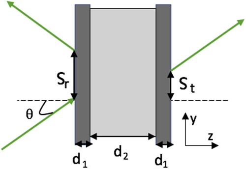
The model consists of three slab layers of uniform dielectrics as depicted in Figure (1). The thickness of the first and last layer is $d_1$ and the middle layer is $d_2$. The permittivity of the edge layers is ${ϵ}_1$ and the intracavity layer is ${ϵ}_2$. The incident light beam of frequency ω attacks the first layer from the vacuum with an angle θ and is assumed to be TE polarized light (A similar treatment can be applied to TM polarized light). We could fill the interactive layer (second layer) with, in principle, any material but here because of our seek to find the general treatment, we will leave it as a free parameter. The permittivity equals ${ϵ}_2=1+\chi =1+{\chi }_r+i{\chi }_i$, where χ is the susceptibility and ${\chi }_r$ [${\chi }_i$] is the real [imaginary] part of the susceptibility.

Figure 1. The slab cavity configuration of three layers. The probe beam enters the cavity with an angle θ, and the reflected and transmitted GHS are denoted as $S_r$ and $S_t$, respectively.

The slab cavity with exactly our description is well-known in the literature (for example [22,24]) and the calculations are mostly performed using the standard characteristic matrix approach [37,38]. The resultant transmission and reflection coefficients applied to our inputs are (1) $\begin{array}{rl}T(k_y,\omega )& =\frac{2q_0}{q_0(Q_{22}+Q_{11})-(q_0^2{Q}_{12}+Q_{21})},\end{array}$(1) (2) $\begin{array}{rl}R(k_y,\omega )& =\frac{q_0(Q_{22}-Q_{11})-(q_0^2{Q}_{12}-Q_{21})}{q_0(Q_{22}+Q_{11})-(q_0^2{Q}_{12}+Q_{21})},\end{array}$(2) where the wavenumber vector is $\mathbf{k}=k_y\hat{\mathbf{j}}+k_z\hat{\mathbf{k}}$. In the vacuum, $k_z=\sqrt{k^2-k_y^2}$, where k is the absolute value of $\mathbf{k}$ which equals $k=\omega /c$, and $q_0$ equals $k_z/k$. The Q elements $Q_{11}$, $Q_{22}$, $Q_{12}$ and $Q_{21}$ are the matrix elements of the following matrix (3) $Q=M_1(k_y,\omega ,d_1)M_2(k_y,\omega ,d_2)M_3(k_y,\omega ,d_1),$(3) where $M_j$ matrix represents each layer in the slab with $d_3=d_1$. The $M_j$ matrices are given as (4) $M_j(\theta ,\omega ,d_j)=\left(\begin{array}{cc}\cos [k_z^j{d}_j]& i\sin [k_z^j{d}_j]/q_j\\ i{q}_j\sin [k_z^j{d}_j]& \cos [k_z^j{d}_j]\end{array}\right),$(4) where $k_z^j=\sqrt{{ϵ}_j{k}^2-k_y^2}$ and $q_j=k_z^j/k$.

Next the lateral shift (GHS), if we assume the broadening of the beam is quite narrow compering to the probe beam $k\gg \mathrm{\Delta }k$, and the beam is well-collimated, the stationary phase theory [5,6,39] can be applied. Thus, the analytic expression of the transmitted and reflected GHS can be expressed as (5) $\begin{array}{rl}\frac{S_t}{\lambda }& =-\frac{1}{\lambda }\frac{\mathrm{d}{\varphi }_t}{d{k}_y}=-\frac{1}{2\pi \cos \theta }\frac{\mathrm{d}{\varphi }_t}{\mathrm{d}\theta },\\ \frac{S_r}{\lambda }& =-\frac{1}{\lambda }\frac{\mathrm{d}{\varphi }_r}{d{k}_y}=-\frac{1}{2\pi \cos \theta }\frac{\mathrm{d}{\varphi }_r}{\mathrm{d}\theta },\end{array}$(5) where ${\varphi }_t$ and ${\varphi }_r$ are the phases of T and R, which can be calculated from (6) ${\varphi }_t={\tan }^{-1}\left(\frac{\mathrm{Im}[T]}{\mathrm{Re}[T]}\right),{\varphi }_r={\tan }^{-1}\left(\frac{\mathrm{Im}[R]}{\mathrm{Re}[R]}\right),$(6) where ($\mathrm{Re}$) is the real value and ($\mathrm{Im}$) is the imaginary value. More detail calculations can be found in many references such as [22,40].

After doing the calculations we can substitute $k_y=k\sin \theta$, so T and R will be directly as a function of the incident angle. The numerical calculation will be performed with the following selected values: $d_1=0.2\mu \mathrm{m}$, $d_2=5\mu \mathrm{m}$, ${ϵ}_1={ϵ}_3=2.22$. The angular frequency of the probe beam is assumed to be fixed and is assumed to be $\omega =(2\pi \times 300\ast {10}^{12}){\mathrm{s}}^{-1}$ with $\lambda =2\pi c/\omega$. Most of these values or similar to them are used in many references such as [22,24,27].

3. The reflection beam

In this section, we will focus on the reflected GHS against the input susceptibility $\chi ={\chi }_r+i{\chi }_i$ and the angle θ.

3.1. ${\chi }_i=0$

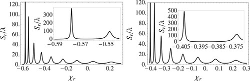
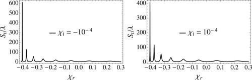
This case corresponds to zero absorption or gain. Let us select two test angles, say $\theta =40$ and $\theta =50$. The reflected GHS for both angles is shown in Figure (2). From the figure, we can observe many peaks. These peaks decrease in height as ${\chi }_r$ increases and their width increases as the susceptibility increases. The number of these peaks seems to be infinite; however, as ${\chi }_r\to \mathrm{\infty }$, they become quite difficult to distinguish, where they become almost a continuous line. Although they seem to be infinite, they have a starting peak which is the longest of them as appear in the figure. For instance, the position of the first peak of $\theta =50$ is located at ${\chi }_r\approx -0.403235$ with a height equals $S_r/\lambda \approx 490.4$. The gap between two consecutive peaks is rising as well as ${\chi }_r$ rises.

Figure 2. The reflected GHS versus the real susceptibility with ${\chi }_i=0$. The angle of the left figure is $\theta =40$, and the angle of the right figure is $\theta =50$.

We also observe that the position of the first peak varies as the angle varies; namely, as the angle goes toward $\theta =90$ as its ${\chi }_r$ increases. From now and on, we are going to call these peaks as modes with being the first mode is the largest of them. Also, we denote the position of these peaks as ${\chi }_r={\chi }_{r,n}(\theta )$, where n is the mode number which take values $n=1,2,3,\dots$. For instance, the first three modes of $\theta =50$ are ${\chi }_{r,1}(50)=-\mathrm{0.403234..}$, ${\chi }_{r,2}(50)=-\mathrm{0.373414..}$, ${\chi }_{r,3}(50)=-\mathrm{0.323773..}$. After studying the analytical expressions of Equations (2(2) $\begin{array}{rl}R(k_y,\omega )& =\frac{q_0(Q_{22}-Q_{11})-(q_0^2{Q}_{12}-Q_{21})}{q_0(Q_{22}+Q_{11})-(q_0^2{Q}_{12}+Q_{21})},\end{array}$(2) ) and (6(6) ${\varphi }_t={\tan }^{-1}\left(\frac{\mathrm{Im}[T]}{\mathrm{Re}[T]}\right),{\varphi }_r={\tan }^{-1}\left(\frac{\mathrm{Im}[R]}{\mathrm{Re}[R]}\right),$(6) ), we found that the zeros of the following equation is approximately yield ${\chi }_{r,n}(\theta )$ (7) $\sin {\left(\frac{\omega }{c}{d}_2\sqrt{1+{\chi }_r-{\sin }^2\theta }\right)}^2=0,$(7) After solving it for ${\chi }_r$, it yields (8) ${\chi }_{r,n}(\theta )\approx {\left(\frac{n\pi c}{\omega d_2}\right)}^2+{\sin }^2\theta -1,$(8) where n takes values $n=1,2,3,\dots$. Although this equation does not provide the accurate value of ${\chi }_{r,n}(\theta )$, it gives a very good approximation. For example, the first three modes of $\theta =50$ from the equation are $-0.40319$, $-0.3732$, $-0.3233$, respectively. These values are very close to the exact values provided above. Another important factor of this simple model of Equation (7(7) $\sin {\left(\frac{\omega }{c}{d}_2\sqrt{1+{\chi }_r-{\sin }^2\theta }\right)}^2=0,$(7) ) is that it can roughly predict the number of peaks when GHS plotted against the incident angle θ. The number of modes is a function of ${\chi }_r$ given as (9) $N_{{\chi }_r}=\frac{\omega }{c}{d}_2\frac{\sqrt{1+{\chi }_r}}{\pi }.$(9) And this, for example, agrees with [22,24] as in Figure 2 in [22], the authors plotted GHS against θ. The value of ${\chi }_r$ in their model for the selected Rabi frequencies is almost constant and equals ${\chi }_r\approx -0.198$. Using our model of Equation (9(9) $N_{{\chi }_r}=\frac{\omega }{c}{d}_2\frac{\sqrt{1+{\chi }_r}}{\pi }.$(9) ) predicts 8.95 peaks, while in the figures of [22] the number of peaks is between 8 to 9 in agreement to this simple model. Another example with nanostructure systems such as [41], where modifying the thickness of the intracavity medium varying the number of peaks in agreement to Equation (9(9) $N_{{\chi }_r}=\frac{\omega }{c}{d}_2\frac{\sqrt{1+{\chi }_r}}{\pi }.$(9) ).

We also find the approximated expression of the height of the modes, the GHS of the modes, which equals (10) $\frac{S_r}{\lambda }\approx \frac{2}{\pi }{\left(\frac{k{d}_2}{n}\right)}^2\sin \theta .$(10) This approximation is only valid for relatively small angles, less than $\theta \approx 60$. However, the ratio between the heights of the modes is almost true for all angles. The heights ratio between two consecutive modes from Equation (10(10) $\frac{S_r}{\lambda }\approx \frac{2}{\pi }{\left(\frac{k{d}_2}{n}\right)}^2\sin \theta .$(10) ) is $(n+1{)}^2/n^2$ which is very close to the correct ratio.

For large angles, the GHS becomes quite large. For example, at angle $\theta =85$, the GHS of the first mode is $S_r/\lambda \approx 3300$ while for angle $\theta =89$, the GHS of the first mode is $\approx 16,000$. Therefore, for this case, ${\chi }_i=0$, giant GHS can only be produced at large angles near $\theta =90$ at ${\chi }_{r,n}(\theta )$ with being the largest GHS values are of the first few modes.

3.2. ${\chi }_i\to 0$

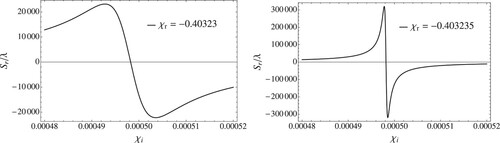
Now, we discuss the dramatic change of the second case when ${\chi }_i$ approaches zero form both directions ±. To take a glance over the GHS for this case, see Figure (3). In the figure, we can see as ${\chi }_i\to 0$ as the heights of the modes start to increase. In this case, when ${\chi }_i$ is positive (negative), the GHS is negative (positive) and quickly becomes giant. When we further increase the limit ${\chi }_i\to 0$ around ${\chi }_i\approx \pm {10}^{-6}$, it becomes clear that these emerging giant shifts do not exactly have the same position as the original modes ${\chi }_{r,n}(\theta )$, instead, they are slightly shifted. The behaviour of GHS around zero has several separated peaks as the behaviour of ${\chi }_i=0$. The GHS, in this case, has a limitless size, it approaches infinite as ${\chi }_i\to 0$ with a bandwidth of the peak goes to zero as well. The number of these giant GHS of a given small ${\chi }_i$ is infinite (always located around the modes), and the heights of these giants are almost the same for a given ${\chi }_i$. Indeed the behaviour of GHS of this case will converge to the original case of $\chi =0$. 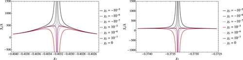To illustrate this fact we plotted the first and second modes in Figure (4) with different small values of ${\chi }_i$. We observe that as $\chi \to 0$ as the emerging peaks become narrower and longer, thus when $\chi =0$ the width of these new peaks become zero and disappear.

Figure 3. The reflected GHS against ${\chi }_r$ for angle $\theta =50$. The black curves are with ${\chi }_i<0$, and the red (dashed) curves are with ${\chi }_i>0$. For a given figure the absolute value of $|{\chi }_i|$ is the same and is indicated under the figure. The bottom left and right figures 1re the same but shown in different scales.

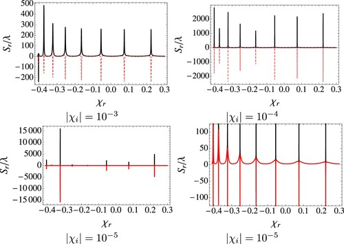
Figure 4. The reflected GHS versus the real susceptibility. The incident angle is $\theta =50$ and the values of ${\chi }_i$ are indicated in the figures. The left (right) figure shows a magnified scale of the first (second) mode.

From this point and on we will name this type of giant GHS as the first type (Type I). This type has an infinite number of modes, thus we will donate their positions by ${\chi }_{r,n}^I(\theta ,{\chi }_i)$, where n is the mode number. To better see some values of ${\chi }_{r,n}^I(\theta ,{\chi }_i)$ along with their heights refer to Table (1). From the table, we see the values of lateral shifts are escalating dramatically as ${\chi }_i\to 0$. And the position of the modes of type I is slightly different from the position of the modes of $\chi =0$ which means ${\chi }_{r,n}(\theta )\approx {\chi }_{r,n}^I(\theta ,{\chi }_i)$. The difference between the two values is in order of ${10}^{-3}$. The main important feature to notice from the table is that while ${\chi }_i$ goes toward zero, the GHS increases dramatically. Moreover, we observe that how these giant GHS are sensitive to tiny differences near the mode values which are mentioned above Equation (7(7) $\sin {\left(\frac{\omega }{c}{d}_2\sqrt{1+{\chi }_r-{\sin }^2\theta }\right)}^2=0,$(7) ).

Table 1. The peaks values of the first two modes of type I for angle $\theta =50$.

${\chi }_i$	${\chi }_{r,1}^I$	$S_{r,1}^I/\lambda$	${\chi }_{r,2}^I$	$S_{r,2}^I/\lambda$
$-{10}^{-3}$	$-\mathrm{0.403238..}$	−240.8	−0.373382..	489.4
${10}^{-3}$	−0.403214..	−79.85	−0.373327..	−161.4
$-{10}^{-4}$	−0.403216..	3049	−0.373339..	2563
${10}^{-4}$	−0.403216..	−2028	−0.373339..	−2322
$-{10}^{-5}$	−0.403216..	24875	−0.373339..	24,523
${10}^{-5}$	−0.403216..	−23894	−0.373339..	−24,277
$-{10}^{-6}$	−0.403216..	244239	−0.373339..	24,4126
${10}^{-6}$	−0.403216..	−243253	−0.373339..	−24,3875

Since all values of ${\chi }_{r,n}^I(\theta ,{\chi }_i)$ converges toward one value as ${\chi }_i$ approaches zero, as evident from the table, we define the independent mode value of type I to be exactly as (11) ${\chi }_{r,n}^I(\theta )=\underset{{\chi }_i\to 0}{lim}{\chi }_{r,n}^I(\theta ,{\chi }_i).$(11) From this definition, at the value ${\chi }_{r,n}^I(\theta )$, and ${\chi }_i\to 0$, the GHS is infinite. Although in practical applications, we do not go to small values of ${\chi }_i$ as this much, it still a small finite value of ${\chi }_i$ will produce a large GHS as Table (1) shows.

The exact determination of the values ${\chi }_{r,n}^I(\theta ,{\chi }_i)$ is in general difficult, but at least we know their values are close to the mode values, and we know that determining the values ${\chi }_{r,n}^I(\theta )$ are easier. We note that as ${\chi }_i\to 0$ at ${\chi }_{r,n}^I(\theta ,{\chi }_i)$ as the reflection coefficient goes to zero, so at ${\chi }_{r,n}^I(\theta )$, the exact value of R is zero. For example, the pairs of the first mode $({\chi }_r,{\chi }_i)\equiv (-0.4032,{10}^{-4})$, the reflection coefficient equals $|R|=0.2505$, while for $({\chi }_r,{\chi }_i)\equiv (-0.4032,{10}^{-5})$, $|R|$ is 0.02045. And a similar phenomenon happens to all modes and all angles. Therefore, we only need to equate the numerator of R to zero with ${\chi }_i=0$ and solve it for χ. This method gives the exact values of ${\chi }_{r,n}^I(\theta )$ with GHS being infinite. Near this value, the values of ${\chi }_{r,n}^I(\theta ,{\chi }_i)$ can be numerically determined. Equating R = 0 gives (12) $q\cos (k{d}_{2}q)+[C_1+q^2{C}_2]\sin (k{d}_{2}q)=0,$(12) where $q=\sqrt{{ϵ}_2-{\sin }^2\theta }=\sqrt{1+\chi -{\sin }^2\theta }$, $k=2\pi /\lambda =\omega /c$, and (13) $\begin{array}{rl}{C}_1& =\frac{q_1[q_0^2{\cos }^2\alpha +q_1^2{\sin }^2\alpha ]}{[q_0^2-q_1^2]\sin (2\alpha )},\end{array}$(13) (14) $\begin{array}{rl}{C}_2& =\frac{-q_1^2{\cos }^2\alpha -q_0^2{\sin }^2\alpha }{[q_0^2-q_1^2]q_1\sin (2\alpha )},\end{array}$(14) where $\alpha =d_{1}k\sqrt{{ϵ}_1-{\sin }^2\theta }$, $q_0=\cos \theta$, and $q_1=\sqrt{{ϵ}_1-{\sin }^2\theta }$. For known values of $d_1$, $d_2$, k, ${ϵ}_1$, ${ϵ}_2$, and for a given θ, the only unknown variable in the equation is χ which is inside q. This Equation (12(12) $q\cos (k{d}_{2}q)+[C_1+q^2{C}_2]\sin (k{d}_{2}q)=0,$(12) ) has an infinite number of roots, so to find the solution of the nth mode, we need to seek the solution near the value of ${\chi }_{r,n}(\theta )$ of Equation (8(8) ${\chi }_{r,n}(\theta )\approx {\left(\frac{n\pi c}{\omega d_2}\right)}^2+{\sin }^2\theta -1,$(8) ). So solving this equation numerically to determine q and consequently χ yields the exact value of Equation (11(11) ${\chi }_{r,n}^I(\theta )=\underset{{\chi }_i\to 0}{lim}{\chi }_{r,n}^I(\theta ,{\chi }_i).$(11) ). This equation can be applied for any angle, any parameter values, etc. For example, the first three mode values of type I for $\theta =50$ for our parameters are (15) $\begin{array}{rl}{\chi }_{r,1}^I(50)& =-\mathrm{0.40321665158..}\\ {\chi }_{r,2}^I(50)& =-\mathrm{0.37333937354..}\\ {\chi }_{r,3}^I(50)& =-\mathrm{0.32354560255..}\end{array}$(15)

The values as can be seen are very close to ${\chi }_{r,n}^I(\theta ,{\chi }_i)$ from Table (1).

3.3. Other giants

After searching over a huge selection of random and systematic choices of $({\chi }_r,{\chi }_i)$ to obtain large GHS, we found another type of giants. We call this new type as type II. In contrast to type I, this type for a given value of ${\chi }_i$ occurs for one particular mode. Therefore, we will denote its modes as (${\chi }_{r,n}^{II}(\theta ),{\chi }_{i,n}^{II}(\theta ))$ or in short ${\chi }_n^{II}(\theta )$, we here need to determine two values to obtain the giant shift. And as type I this type has an infinite number of modes. Demonstrating these giant modes using figures might be difficult, instead, we use Table (2) to show the clear difference between this type and the previous type. In the table, we only specify the peak values, the maximum heights and ${\chi }_r$, of the input ${\chi }_i$ for the first three modes. We see as ${\chi }_i$ grows close to a specific value, giant GHS appears only for one particular mode, in the table is the first mode, and not for the others. A small deviation of the ${\chi }_i$ lets the GHS be negative giants. We can observe that the first mode is escalating very quickly as ${\chi }_r$ and ${\chi }_i$ go toward a specific value, while the other modes almost remain unchanged compering to the first mode. This ensures that this type is different from the previous type.

Table 2. The peaks values of the three modes of angle $\theta =50$ for some input ${\chi }_i$ values.

${\chi }_i$	${\chi }_{r,1}^{II}$	$S_{r,1}^{II}/\lambda$	${\chi }_{r,2}^I$	$S_{r,2}^I/\lambda$	${\chi }_{r,3}^I$	$S_{r,3}^I/\lambda$
0	$-\mathrm{0.403234..}$	490.5	$-\mathrm{0.373414..}$	123.4	$-\mathrm{0.323773..}$	55.43
$-0.0004$	$-\mathrm{0.403235..}$	3092	$-\mathrm{0.373339..}$	763.7	$-\mathrm{0.323545..}$	671.6
$-0.00049$	$-\mathrm{0.403235..}$	30,299	$-\mathrm{0.373345..}$	660.7	$-\mathrm{0.323545..}$	560.7
$-0.00050$	$-\mathrm{0.403235..}$	$-133,405$	$-\mathrm{0.373343..}$	651.8	$-\mathrm{0.323547..}$	550.9
$-0.000498$	$-\mathrm{0.403235..}$	1,358,669	$-\mathrm{0.373343..}$	653.6	$-\mathrm{0.323547..}$	552.8
$-0.000499$	$-\mathrm{0.403235..}$	$-296,582$	$-\mathrm{0.373343..}$	652.7	$-\mathrm{0.323547..}$	551.9
$-0.0004981$	$-\mathrm{0.403235..}$	3,062,939	$-\mathrm{0.373343..}$	653.5	$-\mathrm{0.323547..}$	552.7
$-0.0004982$	$-\mathrm{0.403235..}$	$-11,857,507$	$-\mathrm{0.373343..}$	653.4	$-\mathrm{0.323547..}$	552.7

From the table, we see that the real part of χ is almost untouched while varying ${\chi }_i$. Thus, this suggests plotting the same phenomenon with a fixed value of ${\chi }_r$ versus ${\chi }_i$. The plot is shown in Figure (5) at which we provided two real values. Apparently, we see two giant peaks (negative and positive) emerge as ${\chi }_r$ moves toward a specific value. This value is so close to the mode values ${\chi }_{r,n}$ and ${\chi }_{r,n}^I$ as evident from the table. Therefore, for this type, as we proceed closer toward a specific ${\chi }_n^{II}(\theta )$, as the GHS will be infinite either positive or negative and a tiny deviation from this value will yield a finite amount of GHS. Thus, if we could determine this ultimate value, we could then adjust it a bit to obtain the desire giant value of GHS.

Figure 5. The reflected GHS against ${\chi }_i$ for angle 50 with a fixed value of ${\chi }_r$.

Before exactly spelling how to find this ultimate value of ${\chi }_n^{II}(\theta )$, let us talk about the reflection coefficient for this case. For giants of type II, the reflection coefficient goes toward infinite as $S_r$ goes toward infinite, and this exactly opposite to type I. For example, the value of $|R|$ from the Table 2or the third, fourth and fifth rows for the first mode equals 59.98, 275 and 2778, respectively. Accordingly, to determine the ultimate values of ${\chi }_n^{II}(\theta )$, we need to equate the denominator of R to zero, and thus R becomes infinite which matches this type. The resultant equation is (16) $q\cos (k{d}_{2}q)+[\widetilde{C_1}+q^2\widetilde{C_2}]\sin (k{d}_{2}q)=0,$(16) where (17) $\begin{array}{rl}\widetilde{C_1}& =\frac{q_1[q_0^2{\cos }^2\alpha -q_1^2{\sin }^2\alpha -i{q}_0{q}_1\sin (2\alpha )]}{2i{q}_0{q}_1\cos (2\alpha )+[q_0^2+q_1^2]\sin (2\alpha )},\end{array}$(17) (18) $\begin{array}{rl}\widetilde{C_2}& =\frac{q_1^2{\cos }^2\alpha -q_0^2{\sin }^2\alpha -i{q}_0{q}_1\sin (2\alpha )}{q_1[2i{q}_0{q}_1\cos (2\alpha )+[q_0^2+q_1^2]\sin (2\alpha )]},\end{array}$(18) where q, α, $q_1$, and $q_2$ are the same as of Equation (12(12) $q\cos (k{d}_{2}q)+[C_1+q^2{C}_2]\sin (k{d}_{2}q)=0,$(12) ). For given constant parameters, we only need to solve this equation to find q or more specifically $\chi ={\chi }_r+i{\chi }_i\equiv {\chi }_n^{II}(\theta )$ which is the ultimate value of χ of the second type. Solving this equation numerically can be exactly done as explained for Equation (12(12) $q\cos (k{d}_{2}q)+[C_1+q^2{C}_2]\sin (k{d}_{2}q)=0,$(12) ). Here solving it for angle $\theta =50$ for the first three modes give (19) $\begin{array}{rl}{\chi }_1^{II}(50)& =-\mathrm{0.403235381500..}-i\mathrm{0.0004981794608..}\\ {\chi }_2^{II}(50)& =-\mathrm{0.373414672327..}-i\mathrm{0.00199569587546..}\\ {\chi }_3^{II}(50)& =-\mathrm{0.323716464655..}-i\mathrm{0.00450156011734..}\end{array}$(19) As we can see the first value is pretty close to the value found in Table (2). 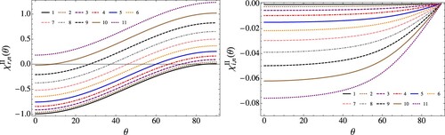Furthermore, we recognize that the real value is extremely close to the mode values ${\chi }_{r,n}$, and the imaginary value of each mode varies from mode to mode. If we solve Equation (16(16) $q\cos (k{d}_{2}q)+[\widetilde{C_1}+q^2\widetilde{C_2}]\sin (k{d}_{2}q)=0,$(16) ) for all angles to obtain ${\chi }_{r,n}^{II}(\theta )$ for the first eleven modes, we would obtain Figure (6). From the figure, we first notice that the real value is almost the same as Type I modes and the modes ${\chi }_{r,n}$, which means if we plot either ${\chi }_{r,n}(\theta )$, or ${\chi }_{r,n}^I(\theta )$, we would see almost the same curves. Another thing is that the imaginary values are always negative which implies that they are always gaining. And this is expected since the reflection will exceed the initial input amplitude, so the media must be gaining.

Figure 6. The real and imaginary values of ${\chi }_n^{II}(\theta )$ for the first 11 modes. The mode number is indicated in the same figures.

This type is found in literature in many articles such as in [22], wherein Figure 3 of this article, they had a relatively high GHS peak around $200\lambda$ for angle $\theta =60$ for both the reflection and transmission GHS. This high shift occurs close to the fifth mode of type II, where the exact value using their parameters gives ${\chi }_5^{II}(60)\approx 0.00032-i0.0109$, and their χ value at that peak is around $\chi =0.001145-i0.00963$. The two values are close to each either, so the peak occurred.

Another thing is that the refractive index of both types can take values starting from near-zero to limitless. To better see this, let us recall the expression of n, the refractive index, for non-magnetic materials $n={ϵ}^2=(1+{\chi }_r+i{\chi }_i{)}^2$. Hence, if ${\chi }_r$ exceeds zero, the refractive index will be larger than one. And in our case, the eleventh mode and the larger modes have values exceeding zero as it is clear from Figure (6).

4. The transmission beam

At first, as we did with the reflection beam, let us see GHS of the transmission beam. We here start from sitting ${\chi }_i=0$ and then start to let ${\chi }_i\to 0$. When ${\chi }_i=0$, the $S_t$ exactly equals $S_r$; the same values and the same behaviour. However, when ${\chi }_i\to 0$, the behaviour starts to differ compering to R. The GHS for some ${\chi }_i$ values are shown in Figure (7). From Figure 1nd further analysis, it appears that the effect of small ${\chi }_i$ is negligible and will not provide giant shifts as the reflected beam. Instead, as ${\chi }_i$ approaches zero as the GHS resembles the normal mode behaviour as Figure (2).

Figure 7. The transmitted GHS versus the real susceptibility. The incident angle is $\theta =50$ and ${\chi }_i=-{10}^{-4}$ for the left Figure and ${\chi }_i={10}^{-4}$ for the right Figure.

We found the only possible way to obtain giant shifts for the transmission light is by applying the same method as the second type. Which is equating the dominator of T to zero, and it will consequently produce infinite GHS and infinite T. The dominator of T is exactly the same as the dominator of R, thus, both have exactly the same values of χ; ${\chi }_n^{II}(\theta )$. Therefore, the transmission shift has only one type which is the second type. And it shares precisely the same susceptibility of the enormous shifts.

5. Discussion and conclusion

We found that the reflected beam has two main types of giant lateral shifts. The first type is at which the reflection tends to be close to zero. According to our understanding, this kind happens because of numerous destructive interferences inside the slab cavity. These destructive interferences lead to attenuate the energy of the reflected beam to become near zero. At meanwhile, since the number of these interferences is huge and has a huge Q factor (Huge number of cycles), these interferences accumulate a sharp and huge change to the phase of the reflected light. And according to Equation (5(5) $\begin{array}{rl}\frac{S_t}{\lambda }& =-\frac{1}{\lambda }\frac{\mathrm{d}{\varphi }_t}{d{k}_y}=-\frac{1}{2\pi \cos \theta }\frac{\mathrm{d}{\varphi }_t}{\mathrm{d}\theta },\\ \frac{S_r}{\lambda }& =-\frac{1}{\lambda }\frac{\mathrm{d}{\varphi }_r}{d{k}_y}=-\frac{1}{2\pi \cos \theta }\frac{\mathrm{d}{\varphi }_r}{\mathrm{d}\theta },\end{array}$(5) ), this will lead to a tremendous GHS. However, the transmission beam does not care about this process and will be almost invariant during ${\chi }_i\to 0$, here is because the transmission is like a halfway interference. It implies that although the reflection suffers from the destruction because of the out of phase frequent full cycles inside the cavity, the transmission only passes through a half cycle so it receives some of the energy without effected by the destruction, and thus will not accumulate as a huge change in phase as the reflection. We also see similar behaviour of T and R of our cavity in other cavities such as the Fabry-Perot cavity [37,42].

The next type (type II) is associated with large reflection and transmission amplitudes. This type, in opposition to the first type, constructively interferes with itself inside the slab cavity. These interferences with a particular finite gaining made the amplitudes quite huge with a huge sharp change in the phase. Here both T and R simultaneously grow to be large. That is because the constructive movements of the half-cycle of T or full-cycle of R build up by a similar fashion. Mathematically speaking, we can see that directly from the expression of both T and R from Equations (1(1) $\begin{array}{rl}T(k_y,\omega )& =\frac{2q_0}{q_0(Q_{22}+Q_{11})-(q_0^2{Q}_{12}+Q_{21})},\end{array}$(1) ) and (2(2) $\begin{array}{rl}R(k_y,\omega )& =\frac{q_0(Q_{22}-Q_{11})-(q_0^2{Q}_{12}-Q_{21})}{q_0(Q_{22}+Q_{11})-(q_0^2{Q}_{12}+Q_{21})},\end{array}$(2) ), where they both share the same denominator. Thus, the action of the gaining, in this type, is equivalent for the transmission and reflection and leads to a large variance for both phases and consequently giant GHS.

Next, we here discuss some of the potential applications of the general expressions of Equations (12(12) $q\cos (k{d}_{2}q)+[C_1+q^2{C}_2]\sin (k{d}_{2}q)=0,$(12) ) and (16(16) $q\cos (k{d}_{2}q)+[\widetilde{C_1}+q^2\widetilde{C_2}]\sin (k{d}_{2}q)=0,$(16) ) of both types. The direct and clear usage is helping researchers to optimize the susceptibility of the intracavity medium to match or avoid, depending on the desire, being equal to one of the modes of the two types. For example, in an atomic medium, the real value of the susceptibility is, say, between $(-0.1,0.1)$, so we properly need to look at the 9th and 10th mode for small angles. And consequently, we need to adjust the gain/absorption of the medium through the external fields to capture one of the modes. Another important application is to apply these relations to other phenomena related to GHS such as the group velocity [24,27] and Gaussian light incident wave [23,25]. The possibilities are tremendous and are beneficial for scientists and engineers.

Testing this model experimentally requires an intracavity medium having full or semi-full control over its susceptibility. A proposal material could be an atomic gas filled by the double-lambda atoms with two external fields [43]. This system can control the optical properties of the material by just adjusting the external fields. Besides, its susceptibility covers a wide range of values. Aside from the intracavity medium, testing this model, especially for the giant GHS values, also requires employing all the explicit and implicit assumptions of the model including, a well-collimated beam, a large slab in y and x-axes, single frequency, etc. Certainly, applying all the assumptions accurately at once is probably challenging. Thus, this work needs to be further studied and it requires simulations and gradually adding the exact experimental environment.

In conclusion, we studied the general treatment of GHS in the slab cavity with general inputs: the incident angle of light and the susceptibility of the intracavity medium. We found that two types are possible to have giant shifts: Type I: with ${\chi }_i\to 0$ and with certain values of ${\chi }_r$, Type II: with certain values of both ${\chi }_r$ and ${\chi }_i$. Type I only appeared in the reflection beam with $R\to 0$ as ${\chi }_r\to {\chi }_{r,n}^I$ and activate all the modes. While Type II appeared in both T and R with $R,T\to \mathrm{\infty }$ and only activate one mode. Negative and positive GHS were found in both types by slightly adjusting the imaginary value of χ.

Acknowledgments

Anas Othman acknowledges financial support from Taibah University. Special thanks to Prof. Mohammed Al-Amri and Dr Saeed Asiri.

Disclosure statement

No potential conflict of interest was reported by the author(s).

References

- Picht J. Beitrag zur Theorie der Totalreflexion. Ann Physik (Paris). 1929;395:433. doi: 10.1002/andp.19293950402
- Goos F, Hänchen H. Ein neuer und fundamentaler Versuch zur Totalreflexion. Ann Phys. 1947;1:333–346. doi: 10.1002/andp.19474360704
- Goos F, Hänchen H. Neumessung des Strahlversetzungseffektes bei Totalreflexion. Ann Phys. 1949;5:251–252. doi: 10.1002/andp.19494400312
- Renard RH. Total reflection: a new evaluation of the Goos–Hänchen shift. J Opt Soc Am. 1964;54:1190. doi: 10.1364/JOSA.54.001190
- Li C-F. Negative lateral shift of a light beam transmitted through a dielectric slab and interaction of boundary effects. Phys Rev Lett. 2003;91:133903.
- Artmann K. Berechnung der Seitenversetzung des totalreflektierten Strahles. Ann Phys. 1948;2:87–102. doi: 10.1002/andp.19484370108
- Hashimoto T, Yoshino T. Optical heterodyne sensor using the Goos–Hänchen shift. Opt Lett. 1989;14:913. doi: 10.1364/OL.14.000913
- Harrick NJ. Study of physics and chemistry of surfaces from frustrated total internal reflections. Phys Rev Lett. 1960;4:224–226. doi: 10.1103/PhysRevLett.4.224
- Birman JL, Pattanayak DN, Puri A. Prediction of a resonance-Enhanced laser-Beam displacement at total internal reflection in semiconductors. Phys Rev Lett. 1983;50:1664. doi: 10.1103/PhysRevLett.50.1664
- Oh G-Y, Kim DG, Choi Y-W. The characterization of GH shifts of surface plasmon resonance in a waveguide using the FDTD method. Opt Express. 2009;17:20714. doi: 10.1364/OE.17.020714
- Lotsch HKV. Beam displacement at total reflection : The Goos-Hanchen effect I. Optik (Jena). 1970;32:116.
- Lotsch HKV. Beam displacement at total reflection : The Goos-Hanchen effect II. Optik (Jena). 1970;32:189.
- Lotsch HKV. Beam displacement at total reflection : The Goos-Hanchen effect III. Optik (Jena). 1971;32:299.
- Lotsch HKV. Beam displacement at total reflection : The Goos-Hanchen effect IV. Optik (Jena). 1971;32:553.
- Wild WJ, Giles CL. Goos-Hänchen shifts from absorbing media. Phys Rev A. 1982;25:2099–2101. doi: 10.1103/PhysRevA.25.2099
- Lai HM, Chan SW. Large and negative Goos–Hänchen shift near the brewster dip on reflection from weakly absorbing media. Opt Lett. 2002;27:680. doi: 10.1364/OL.27.000680
- Felbacq D, Moreau A, Smaâli R. Goos–Hänchen effect in the gaps of photonic crystals. Opt Lett. 2003;28:1633. doi: 10.1364/OL.28.001633
- Wang LG, Zhu SY. Giant lateral shift of a light beam at the defect mode in one-dimensional photonic crystals. Opt Lett. 2006;31:101. doi: 10.1364/OL.31.000101
- Chen X, Wei R-R, Shen M, et al. Bistable and negative lateral shifts of the reflected light beam from kretschmann configuration with nonlinear left-handed metamaterials. Appl Phys B. 2010;101:283–289. doi: 10.1007/s00340-010-4071-1
- Chen X, Ban Y, Li C-F. Voltage-tunable lateral shifts of ballistic electrons in semiconductor quantum slabs. J Appl Phys. 2009;105:093710.
- Chen X, Lu X-J, Wang Y, et al. Controllable Goos–Hänchen shifts and spin beam splitter for ballistic electrons in a parabolic quantum well under a uniform magnetic field. Phys Rev B. 2011;83:195409.
- Wang L-G, Ikram M, Zubairy MS. Control of the Goos-Hänchen shift of a light beam via a coherent driving field. Phys Rev A. 2008;77:023811.
- Ziauddin, Qamar S. Control of the Goos-Hänchen shift using a duplicated two-level atomic medium. Phys Rev A. 2012;85:055804. doi: 10.1103/PhysRevA.85.055804
- Ziauddin, Qamar S, Zubairy M. Coherent control of the Goos–Hänchen shift. Phys Rev A. 2010;81:023821. doi: 10.1103/PhysRevA.81.023821
- Asiri S., Xu J., Al-Amri M., et al. Controlling the Goos-Hänchen and Imbert-Fedorov shifts via pump and driving fields. Phys Rev A. 2016;93:013821.
- Zhang X-J, Wang H-H, Liu C-Z, et al. Controlling transverse shift of the reflected light via high refractive index with zero absorption. Opt Express. 2017;25:10335. doi: 10.1364/OE.25.010335
- Hamedi HR, Radmehr A, Sahrai M. Manipulation of Goos-Hänchen shifts in the atomic configuration of mercury via interacting dark-state resonances. Phys Rev A. 2014;90:053836. doi: 10.1103/PhysRevA.90.053836
- Solookinejad Gh, Jabbari M, Panahi M, et al. Polarized control of Goos–Hänchen shifts in four-level quantized graphene nanostructures. Laser Phys. 2017;27:015204.
- Han P, Chang X, Li W, et al. Tunable Goos–Hänchen shift and polarization beam splitting through a cavity containing double ladder energy level system. IEEE Photonics J. 2019;11:6101013.
- Jafarzadeh H, Payravi M. Theoretical investigation of tunable Goos–Hänchen shifts in a four-Level quantum system. Int J Theor Phys. 2018;57:2415. doi: 10.1007/s10773-018-3763-x
- Asadpour SH, Hamedi HR, Jafari M. Enhancement of Goos–Hänchen shift due to a rydberg state. Appl Opt. 2018;57:4013. doi: 10.1364/AO.57.004013
- Solookinejad Gh, Masoud J, Panahi M, et al. Phase manipulation of Goos–Hänchen shifts in a single-layer of graphene nanostructure under strong magnetic field. Laser Phys. 2017;27:115204.
- Yang W-X. Tunneling-induced giant Goos–Hänchen shift in quantum wells. Opt Lett. 2015;40:3133. doi: 10.1364/OL.40.003133
- Jing Q, Du C, Lei F, et al. Coherent control of the Goos–Hänchen shift via an inhomogeneous cavity. J Opt Soc Am B. 2015;32:1532. doi: 10.1364/JOSAB.32.001532
- Malik A, Chaung YL, Abbas M, et al. Giant negative and positive Goos–Hänchen shifts via doppler broadening effect. Laser Phys. 2019;29:075201. doi: 10.1088/1555-6611/ab14ec
- Luo C, Dai X, Xiang Y. Enhanced and Tunable Goos–Hänchen Shift in a Cavity Containing Colloidal Ferrofluids. IEEE Photonics J. 2015;7: 6100310.
- Born M, Wolf E. Principles of optics. 7th ed.. Cambridge: Cambridge University Press; 1999.
- Liu NH, Zhu SY, Chen H, et al. Superluminal pulse propagation through one-dimensional photonic crystals with a dispersive defect. Phys Rev E. 2002;65:046607.
- Orfanidis SJ. Electromagnetic Waves and Antennas [Online]. Available from: http://eceweb1.rutgers.edu/orfanidi/ewa/ (2013)
- Wang LG, Chen H, Zhu SY. Large negative Goos–Hänchen shift from a weakly absorbing dielectric slab. Opt Lett. 2005;30:2936. doi: 10.1364/OL.30.002936
- Jafarzadeh H. Goos–Hänchen shift via refractive index control of four-level quantum dot nanostructure. Opt Appl. 2018;48(3). doi:10.5277/oa180314.
- Yariv A, Yeh P. Photonics. 6th ed. New York (NY): Oxford University Press; 2007.
- Othman A, Yevick D, Al-Amri M. Generation of three wide frequency bands within a single white-light cavity. Phys Rev A. 2018;97:043816. doi: 10.1103/PhysRevA.97.043816