Bayesian and non-Bayesian reliability estimation of multicomponent stress–strength model for unit Weibull distribution

ABSTRACT

Mazucheli et al. introduced a new transformed model referred as the unit-Weibull (UW) distribution with uni- and anti-unimodal, decreasing and increasing shaped density along with bathtub shaped, constant and non-decreasing hazard rates. Here we consider inference upon stress and strength reliability using different statistical procedures. Under the framework that stress–strength components follow UW distributions with a known shape, we first estimate multicomponent system reliability by using four different frequentist methods. Besides, asymptotic confidence intervals (CIs) and two bootstrap CIs are obtained. Inference results for the reliability are further derived from Bayesian context when shape parameter is known or unknown. Unbiased estimation has also been considered when common shape is known. Numerical comparisons are presented using Monte Carlo simulations and in consequence, an illustrative discussion is provided. Two numerical examples are also presented in support of this study.

Significant conclusion: We have investigated inference upon a stress–strength parameter for UW distribution. The four frequentist methods of estimation along with Bayesian procedures have been used to estimate the system reliability with common parameter being known or unknown.

Keywords:

• Bayesian point and interval procedures
• least square estimator
• stress–strength reliability
• maximum product of spacing estimator

1. Introduction

Many physical phenomena from different disciplines are often modelled using some known probability models which include, among others, Burr family of distributions, lognormal, gamma, exponential, Weibull distributions. These probability distributions can model a variety of data exhibiting significant variability. One particular probability model of specific significance is the well-known Weibull distribution. Over the last five decades or so, several new modifications of this particular model have been proposed and studied by many researchers, such as exponentiated Weibull [1–3], extended Weibull [4,5], modified Weibull [6–8], odd Weibull [9], Weibull-X class [10], Weibull-G model [11], extended Weibull-G family [12] and so on. These distributions are generally derived by adding some additional parameters to the original probability distribution under consideration. Besides, most of these generalizations share one interesting characteristic that they are based on the support over positive part of the real line. Such inferential trend often leads to insufficient number of distributions with finite support. But at the same time, probability distributions with support on finite range are also of importance in many studies. Physical characteristics of many life test experiments quite often lead to data which may lie in some finite range. Data on fractions, percentages, per capita income growth, fuel efficiency of vehicles, height and weight of individuals, survival times from a deadly disease etc. are likely to lie in some bounded positive intervals. Kumaraswamy [13] studied a two-parameter distribution with support on finite interval and investigated many useful applications of this distribution in meteorological inference. Mazucheli et al. [14,15] derived some useful classical estimates for unknown parameters of a unit-gamma distribution and also introduced unit Birnbaum–Saunders distribution, besides, different estimation methods are used to estimate the model parameters. Further, Mazucheli et al. [16] developed and studied properties of a unit Gompertz distribution and derived inferences for its unknown parameters. Mazucheli et al. [17] initially studied various characteristics of a unit Weibull distribution. Through several applications they showed that this particular model can be treated as an useful alternative to the Kumaraswamy and beta distributions in life test studies. We, here, consider multicomponent reliability estimation under unit Weibull probability distribution. This distribution can assume different shapes – monotonic, unimodal, anti-unimodal based on model parameters and such flexibility makes it quite suitable for fitting various data arising in reliability analysis and industrial experiments.

Traditionally, a system consisting more than one component is referred to as multicomponent system, see [18,19]. Under this framework, a system with k independent strength components $X_1,X_2,\dots ,X_k$ properly functions if at least s−out−of−k ($s\le k)$ strength variables exceed the stress Y. Such a system is often called as (“s−out−of−k:G”) system. Physical aspects of many investigations may lead to multi-component systems and many such examples abound in practice. Such structures are extensively utilized in industrial experiments, military radio networks, bridge construction, building communication networks, etc. In recent past, many scholars have studied multicomponent stress–strength models largely owing to the growing interest on this topic, see for instance, works of [20–23], Dey and Moala [24] and many others. Seadawy et al. [25], Seadawy et al. [26], Ahmad et al. [27], Riaz et al. [28], Abbasi et al. [29] have also studied some complex structures.

The probability distribution of a unit Weibull distribution, with range in the interval $(0,1)$, is given by (1) $\begin{array}{rl}{f}_X(x,\alpha ,\text{β})& =\alpha \text{β}(-\ln x{)}^{\text{β}-1}{x}^{-1}{e}^{-\alpha (-\ln x{)}^{\text{β}}},\\ & \alpha >0,\text{β}>0\end{array}$(1) and (2) $F_X\left(x\right)=e^{-\alpha (-\ln x{)}^{\text{β}}},\alpha >0,\text{β}>0,$(2) where $\alpha ,\text{β}$ govern shape of UW distribution. We write this distribution as $UW(\alpha ,\text{β})$.

Various frequentist procedures are discussed to estimate the unknown multicomponent reliability function. We further estimate this unknown parametric function using Bayes procedure against proper and improper prior distributions under a well-known loss function. Next, we have constructed asymptotic, two bootstrap and HPD intervals. Further, UMVUE of the multicomponent reliability is discussed as well under the case that common shape is known. To the our knowledge, this estimation problem based on unit Weibull distribution is not discussed before using the aforementioned methods of estimation.

Contribution of this work is many fold as UW distribution has not been discussed much in the literature. We derive inference for $R_{s,k}$ under various classical methods like maximum likelihood estimator (MLE), least square estimator (LSE) and weighted LSE (WLSE) and maximum product of spacing (MPS) estimators. These estimators are evaluated against estimated risks and average bias values computed using various sample sizes. We further estimate $R_{s,k}$ by Bayesian method based on proper and improper priors. Interval estimation is taken care as well. We have constructed asymptotic interval, bootstrap intervals and highest posterior density (HPD) interval. We compare these estimates using their length and coverage probabilities. The uniformly minimum variance unbiased estimator (UMVUE) of $R_{s,k}$, with known common scale, is derived as well. Our aim is to provide a guideline for selecting the better inference procedure among different classical and Bayesian methods. This would be of deep interest to reliability engineers.

The reliability of system is briefly illustrated in Section 2. In the same section, we describe four classical estimation methods, namely, MLE, LSE, WLSE and MPS to estimate multicomponent reliability and construct asymptotic and two bootstrap (boot−t and boot−p) CIs of multicomponent reliability when all parameters of the system are unknown. Further Bayes estimator is discussed when the prior distributions of β, ${\alpha }_1$ and ${\alpha }_2$ are gamma variables and also independent. In sequel, the HPD interval of multicomponent reliability is also constructed. Subsequently in Section 3, frequentist and Bayesian inference of multicomponent reliability are derived under the assumption that β is known. Simulations results are evaluated in Section 4 to examine numerical performance of proposed procedures. Two real-life examples are studied in Section 5. Finally, paper is concluded in Section 6.

2. Inference for $R_{s,k}$ with unknown β

Suppose $X_1,X_2,\dots ,X_k$ denote strength components with cdf as given in (2(2) $F_X\left(x\right)=e^{-\alpha (-\ln x{)}^{\text{β}}},\alpha >0,\text{β}>0,$(2) ). Likewise variable Y denotes associated stress acting on the system with distribution function $G_Y(y;{\alpha }_2,\text{β})$. Then we have (see Rao et al. [19]) (3) $\begin{array}{rl}{R}_{s,k}& =\sum _{i=s}^k\left(\genfrac{}{}{0ex}{}{k}{i}\right){\int }_{-\mathrm{\infty }}^{\mathrm{\infty }}(1-F({\alpha }_2,\text{β},y){)}^i\\ & \times \left(F\right({\alpha }_2,\text{β},y\left){)}^{k-i}\mathrm{d}G\right(y).\end{array}$(3) We next derive some useful inference of this parametric function using different procedures when common shape is unknown or known.

2.1. MLE of $R_{s,k}$

Suppose that $X_1,X_2,\dots ,X_k$ are taken from $UW({\alpha }_1,\text{β})$ distribution and Y follows a $UW({\alpha }_2,\text{β})$ distribution where parameters ${\alpha }_1,{\alpha }_2$ and β are assumed as unknown. Under this framework, we get that $\begin{array}{rl}{R}_{s,k}& ={\alpha }_1\text{β}\sum _{i=s}^k\left(\genfrac{}{}{0em}{}{k}{i}\right){\int }_0^{\mathrm{\infty }}{\left(1-e^{-{\alpha }_1(-\ln y{)}^{\text{β}}}\right)}^i\\ & \times {\left(e^{-{\alpha }_1(-\ln y{)}^{\text{β}}}\right)}^{k-i}\\ & \times {\alpha }_2\text{β}(-\ln y{)}^{\text{β}-1}{y}^{-1}{e}^{-{\alpha }_2(-\ln y{)}^{\text{β}}}\mathrm{d}y.\end{array}$ After some simplification, we have (4) $R_{s,k}=\sum _{i=s}^k\sum _{j=0}^i(-1{)}^j\left(\genfrac{}{}{0em}{}{i}{j}\right){\alpha }_2\left(\genfrac{}{}{0em}{}{k}{i}\right)[{\alpha }_1(j+k-i)+{\alpha }_2{]}^{-1}.$(4) We proceed by assuming that n structures are subjected to a test. The likelihood, based on observed data $x_{i1},x_{i2},\dots ,x_{ik}$ and $y_i$, of $({\alpha }_1,{\alpha }_2,\text{β})$ is $\begin{array}{rl}& L\left({\alpha }_1,{\alpha }_2,\text{β};x,y\right)\\ & =\prod _{i=1}^n\left(\prod _{j=1}^k\left({\alpha }_1\text{β}(-\ln x_{ij}{)}^{\text{β}-1}{x}_{ij}^{-1}{e}^{-{\alpha }_1(-\ln x_{ij}{)}^{\text{β}}}\right)\right)\\ & \times \left({\alpha }_2\text{β}(-\ln y_i{)}^{\text{β}-1}{y}_i^{-1}{e}^{-{\alpha }_2(-\ln y_i{)}^{\text{β}}}\right).\end{array}$ The log-likelihood turns out to be (5) $\begin{array}{rl}& l\left({\alpha }_1,{\alpha }_2,\text{β};x,y\right)\\ & =(\log {\alpha }_1)\left(nk\right)+\sum _{i=1}^n\sum _{j=1}^k\log \left(1/x_{ij}\right)\\ & +(\text{β}-1)\sum _{i=1}^n\sum _{j=1}^k\log (-\log x_{ij})\\ & -{\alpha }_1\sum _{i=1}^n\sum _{j=1}^k(-\log x_{ij}{)}^{\text{β}}\\ & +\sum _{i=1}^n\log \left(1/y_i\right)+(\text{β}-1)\sum _{i=1}^n\log (-\log y_i)\\ & +(\log \text{β})\left(n\right(k+1\left)\right)\\ & -{\alpha }_2\sum _{i=1}^n(-\log y_i{)}^{\text{β}}+(\log {\alpha }_2)n.\end{array}$(5) Partially differentiating the loglikelihood, respectively, w.r.t ${\alpha }_1$, ${\alpha }_2$ and β and equating to zero yield following results.

The MLE ${\hat{\alpha }}_1$ of ${\alpha }_1$ is (6) ${\hat{\alpha }}_1=\frac{nk}{{\displaystyle \sum _{i=1}^n\sum _{j=1}^k(-\log x_{ij}{)}^{\text{β}}}}.$(6) Similarly, from $\frac{\mathrm{\partial }l}{\mathrm{\partial }{\alpha }_2}=\frac{n}{{\alpha }_2}-\sum _{i=1}^n(-\log y_i{)}^{\text{β}}=0,$ we get the MLE ${\hat{\alpha }}_2$ of ${\alpha }_2$ as (7) ${\hat{\alpha }}_2=\frac{n}{{\displaystyle \sum _{i=1}^n(-\log y_i{)}^{\text{β}}}}.$(7) Finally, $\mathrm{\partial }l/\mathrm{\partial }\text{β}=0$ is solved for β to obtain its MLE $\widehat{\text{β}}$ satisfying (8) $\begin{array}{rl}& \frac{(nk+n)}{\widehat{\text{β}}}+\sum _{i=1}^n\sum _{j=1}^k\log (-\log x_{ij})+\sum _{i=1}^n\log (-\log y_i)\\ & -{\hat{\alpha }}_1\sum _{i=1}^n\sum _{j=1}^k\log (-\log x_{ij})(-\log x_{ij}{)}^{\text{β}}\\ & -{\hat{\alpha }}_2\sum _{i=1}^n\log (-\log y_i)(-\log y_i{)}^{\text{β}}=0.\end{array}$(8) The above likelihood equation is nonlinear and can be solved numerically using some iterative technique. Plugging MLE of β in Equations (6(6) ${\hat{\alpha }}_1=\frac{nk}{{\displaystyle \sum _{i=1}^n\sum _{j=1}^k(-\log x_{ij}{)}^{\text{β}}}}.$(6) ) and (7(7) ${\hat{\alpha }}_2=\frac{n}{{\displaystyle \sum _{i=1}^n(-\log y_i{)}^{\text{β}}}}.$(7) ), we can obtain $\widehat{{\alpha }_1}$ and $\widehat{{\alpha }_2}$, respectively. Now MLE ${\hat{R}}_{s,k}$ of $R_{s,k}$ turns out to be $R_{s,k}=\sum _{i=s}^k\sum _{j=0}^i(-1{)}^j{\hat{\alpha }}_2\left(\genfrac{}{}{0em}{}{i}{j}\right)\left(\genfrac{}{}{0em}{}{k}{i}\right)[{\hat{\alpha }}_1(j+k-i)+{\hat{\alpha }}_2{]}^{-1}.$

2.2. Asymptotic interval

Here a confidence interval of the multicomponent reliability is given using MLE. The Fisher information of $\theta =({\alpha }_1,{\alpha }_2,\text{β})$ is $I\left(\theta \right)=-\left[\begin{array}{ccc}{I}_{11}& I_{12}& I_{13}\\ I_{21}& I_{22}& I_{23}\\ I_{31}& I_{32}& I_{33}\end{array}\right].$ The elements of $I\left(\theta \right)$ are $\begin{array}{rl}{I}_{11}& =E\left(\frac{{\mathrm{\partial }}^{2}l}{\mathrm{\partial }{\alpha }_1^2}\right)=-\frac{nk}{{\alpha }_1^2},I_{22}=E\left(\frac{{\mathrm{\partial }}^{2}l}{\mathrm{\partial }{\alpha }_2^2}\right)=-\frac{n}{{\alpha }_2^2},\\ I_{12}& =I_{21}=E\left(\frac{{\mathrm{\partial }}^{2}l}{{\mathrm{\partial }}_1{\alpha }_1\mathrm{\partial }{\alpha }_2}\right)=0,\\ I_{13}& =I_{31}=E\left(\frac{{\mathrm{\partial }}^{2}l}{\mathrm{\partial }{\alpha }_1\mathrm{\partial }\text{β}}\right)\\ & =nk{\int }_0^1\log (-\log x_{ij})(-\log x_{ij}{)}^{\text{β}}{\alpha }_1\\ & \times \text{β}(-\ln x_{ij}{)}^{\text{β}-1}{x}_{ij}^{-1}{e}^{-{\alpha }_1(-\ln x_{ij}{)}^{\text{β}}}\mathrm{d}{x}_{ij}.\end{array}$ After some simplification, we get $I_{13}=I_{31}=-\frac{nk}{{\alpha }_1\text{β}}{\int }_0^{\mathrm{\infty }}u{e}^{-u}\log \left(u/{\alpha }_1\right)\mathrm{d}u.$ Similarly, we have $I_{23}=I_{32}=-\frac{n}{{\alpha }_2\text{β}}{\int }_0^{\mathrm{\infty }}u{e}^{-u}\log \left(u/{\alpha }_2\right)\mathrm{d}u$ and $\begin{array}{rl}{I}_{33}& =-\frac{n(k+1)}{{\text{β}}^2}-\frac{nk}{{\text{β}}^2}{\int }_0^{\mathrm{\infty }}u{e}^{-u}(\log (u/{\alpha }_1){)}^2\mathrm{d}u\\ & -\frac{n}{{\text{β}}^2}{\int }_0^{\mathrm{\infty }}u{e}^{-u}(\log (u/{\alpha }_2){)}^2\mathrm{d}u.\end{array}$ From the large sample theory, the MLE of reliability is normal with average given by $R_{s,k}$. The associated variance is computed as $\begin{array}{rl}{\sigma }_{R_{s,k}}^2& ={\left(\frac{\mathrm{\partial }{R}_{s,k}}{\mathrm{\partial }{\alpha }_1}\right)}^2{I}_{11}^{-1}+{\left(\frac{\mathrm{\partial }{R}_{s,k}}{\mathrm{\partial }{\alpha }_2}\right)}^2{I}_{22}^{-1}\\ & +2\left(\frac{\mathrm{\partial }{R}_{s,k}}{\mathrm{\partial }{\alpha }_1}\right)\left(\frac{\mathrm{\partial }{R}_{s,k}}{\mathrm{\partial }{\alpha }_2}\right)I_{12}^{-1},\end{array}$ where we have $\begin{array}{rl}\frac{\mathrm{\partial }{R}_{s,k}}{\mathrm{\partial }{\alpha }_1}& =\sum _{i=s}^k\sum _{j=0}^i(j+k-i)\left(\genfrac{}{}{0ex}{}{k}{i}\right)\left(\genfrac{}{}{0ex}{}{i}{j}\right)(-1{)}^{j+1}{\alpha }_2\\ & \times {\left[{\alpha }_1(j+k-i)+{\alpha }_2\right]}^{-2}\end{array}$ and similarly $\mathrm{\partial }{R}_{s,k}/\mathrm{\partial }{\alpha }_2$ is evaluated. Thus $100(1-\eta )\mathrm{\%}$ CI of the parametric function is given by $({\hat{R}}_{s,k}\pm q_{\eta /2}{\hat{\sigma }}_{R_{s,k}})$, where $q_{\eta /2}$ is associated percentile of normal $N(0,1)$ variable and ${\hat{\sigma }}_{R_{s,k}}$ is computed at respective MLEs.

2.3. Bootstrapping

We develop boot-p and boot-t intervals for $R_{S,k}$ (see Efron [30] and Hall [31] for further details).

2.3.1. Boot-p

1. Obtain samples $(y_1^{\ast },\dots ,y_n^{\ast })$ of size n and also simulate $(x_{i1}^{\ast },\dots ,x_{ik}^{\ast })$ of size nk where i is a positive integer ranging from 1 to n. Based on it, a sample estimate of reliability is computed as ${\hat{R}}_{s,k}^{\ast }$.

2. Iterate above stage, say nboot times.

3. Now if $F^{\ast }\left(x\right)=P({\hat{R}}_{s,k}^{\ast }\le x)$ denote cdf of ${\hat{R}}_{s,k}^{\ast }$ and assume that ${\hat{R}}_{s,k}^{bp}\left(x\right)=F^{\ast -1}\left(x\right)$ for a given x. Then $100(1-\eta )\mathrm{\%}$ boot-p interval is computed as $\left({\hat{R}}_{s,k}^{bp}\right(\eta /2),{\hat{R}}_{s,k}^{bp}(1-\left(\eta /2\right)\left)\right).$

2.3.2. Boot-t

1. Simulate bootstrap samples $(y_1^{\ast },\dots ,y_n^{\ast })$ of size n and also generate $(x_{i1}^{\ast },\dots ,x_{ik}^{\ast })$ of size nk where i is a positive integer ranging from 1 to n. Based on it, a sample estimate of reliability is computed as ${\hat{R}}_{s,k}^{\ast }$.

2. Evaluate $T^{\ast }=\left(\sqrt{V\left({\hat{R}}_{s,k}^{\ast }\right)}{)}^{-1}\right({\hat{R}}_{s,k}^{\ast }-{\hat{R}}_{s,k})$.

3. Iterate above two stages sufficient number of times.

4. Suppose $H_{T^{\ast }}\left(x\right)$ is cdf of variable as defined in Step 2 and define ${\hat{R}}_{s,k}^{bt}\left(x\right)={\hat{R}}_{s,k}\left(x\right)+\left[H_{T^{\ast }}^{-1}\right(x\left)\right]\left[\sqrt{V\left({\hat{R}}_{s,k}\right)}\right].$ Then $100(1-\eta )\mathrm{\%}$ boot-t interval is computed as $\left({\hat{R}}_{s,k}^{bt}\right(\eta /2),{\hat{R}}_{s,k}^{bt}(1-\left(\eta /2\right)\left)\right).$

2.4. Least square and weighted least square estimates

The LSE method is initially discussed by Swain et al. [32]. Here we obtain this estimator for the multicomponent reliability $R_{s,k}$. Note that LSE ${\widehat{{\alpha }_1}}^L$ of ${\alpha }_1$ can be computed by minimizing $\sum _{i=1}^{nk}\left[F_X\right(x_i)-(i/(nk+1)){]}^2$, that is, $\sum _{i=1}^{nk}[e^{-{\alpha }_1(-\ln x_i{)}^{\text{β}}}-(i/(nk+1)){]}^2$. So LSE ${\hat{\alpha }}_1^l$ is the solution of the following equation: $\begin{array}{rl}& \sum _{i=1}^{nk}[e^{-{\hat{\alpha }}_1^l(-\ln x_i{)}^{\text{β}}}-(i/(nk+1)\left)\right]\\ & \times e^{-{\hat{\alpha }}_1^l(-\ln x_i{)}^{\text{β}}}(-\ln x_i{)}^{\text{β}}=0,\end{array}$ where $X_1,X_2,\dots ,X_{nk}$ follow $UW({\alpha }_1,\text{β})$ distribution. The LSE ${\widehat{{\alpha }_2}}_L$ of ${\alpha }_2$ is computed similarly by solving the following equation: $\begin{array}{rl}& \sum _{i=1}^n[e^{-{\hat{\alpha }}_2^l(-\ln y_i{)}^{\text{β}}}-(i/(nk+1)\left)\right]\\ & \times e^{-{\hat{\alpha }}_2^l(-\ln y_i{)}^{\text{β}}}(-\ln y_i{)}^{\text{β}}=0,\end{array}$ where $Y_1,Y_2,\dots ,Y_n$ follow $UW({\alpha }_2,\text{β})$ distribution. Thus LSE of $R_{s,k}$ turns out to be ${\hat{R}}_{s,k}^l=\sum _{i=s}^k{\hat{\alpha }}_2^l\sum _{j=0}^i\left(\genfrac{}{}{0em}{}{k}{i}\right)\left(\genfrac{}{}{0em}{}{i}{j}\right)\left[{\hat{\alpha }}_1^l\right(j+k-i)+{\hat{\alpha }}_2^l{]}^{-1}(-1{)}^j.$ Next, weighted least square estimates (WLSE) ${\hat{\alpha }}_1^w$ of ${\alpha }_1$ is computed by minimizing the following function: $\sum _{i=1}^{nk}\frac{(nk+1{)}^2(nk+2)}{i(nk-i+1)}[e^{-{\alpha }_1(-\ln x_i{)}^{\text{β}}}-(i/(nk+1)){]}^2$ and thus the required estimate is determined from the following equation: $\begin{array}{rl}& \sum _{i=1}^{nk}\frac{(nk+1{)}^2(nk+2)}{i(nk-i+1)}[e^{-{\hat{\alpha }}_1^w(-\ln x_i{)}^{\text{β}}}-(i/(nk+1)\left)\right]\\ & \times e^{-{\hat{\alpha }}_1^w(-\ln x_i{)}^{\text{β}}}(-\ln x_i{)}^{\text{β}}=0.\end{array}$ The WLSE estimate ${\hat{\alpha }}_2^w$ of ${\alpha }_2$ is similarly computed from the equation presented below: $\begin{array}{rl}& \sum _{i=1}^n\frac{(n+1{)}^2(n+2)}{i(n-i+1)}[e^{-{\hat{\alpha }}_2^w(-\ln y_i{)}^{\text{β}}}-(i/(nk+1)\left)\right]\\ & \times e^{-{\hat{\alpha }}_2^w(-\ln y_i{)}^{\text{β}}}(-\ln y_i{)}^{\text{β}}=0.\end{array}$ So WLSE of $R_{s,k}$ is given by ${\hat{R}}_{s,k}^w=\sum _{i=s}^k\sum _{j=0}^i\left(\genfrac{}{}{0em}{}{k}{i}\right)\left(\genfrac{}{}{0em}{}{i}{j}\right)\frac{(-1{)}^j{\hat{\alpha }}_2^w}{{\hat{\alpha }}_1^w(j+k-i)+{\hat{\alpha }}_2^w}.$

2.5. Maximum product of spacing (MPS) estimates

Here we obtain another estimator called MPS estimates of the multicomponent reliability as discussed in [33]. Here spacing of a random sample of size nk is defined as $D_i\left({\alpha }_1\right)=F_X\left(x_i\right)-F_X\left(x_{i-1}\right),i=1,2,\dots ,nk,$ also $F_X\left(x_0\right)=0$ and $F_X\left(x_{nk+1}\right)=1$. The desired estimate ${\hat{\alpha }}_1^m$ of ${\alpha }_1$ is computed by maximizing the geometric mean $\left(\prod _{i=1}^{nk+1}{D}_i\right({\alpha }_1){)}^{1/(nk+1)}$ of spacing. Alternatively we maximize $\left(1/\right(nk+1\left)\right)\sum _{i=1}^{nk+1}\ln D_i\left({\alpha }_1\right)$ and compute the desired estimate of ${\alpha }_1$ from the following equation: $\begin{array}{rl}& \left(1/\right(nk+1\left)\right)\sum _{i=1}^{nk+1}\frac{1}{D_i\left({\hat{\alpha }}_1^m\right)}[-e^{-{\hat{\alpha }}_1^m(-\ln x_i{)}^{\text{β}}}(-\ln x_i{)}^{\text{β}}\\ & +e^{-{\hat{\alpha }}_1^m(-\ln x_{i-1}{)}^{\text{β}}}(-\ln x_i{)}^{\text{β}}]=0.\end{array}$ Next using a sample of size n from the Y variable, define $D_i^{\ast }\left({\alpha }_2\right)=F_Y\left(y_i\right)-F_Y\left(y_{i-1}\right),i=1,2,\dots ,n,$ also $F_Y\left(y_0\right)=0$ and $F_Y\left(y_{n+1}\right)=1$. The MPS estimate ${\hat{\alpha }}_2^m$ of ${\alpha }_2$ is determined from equation presented as $\begin{array}{rl}& \left(1/\right(n+1\left)\right)\sum _{i=1}^{n+1}\frac{1}{D_i^{\ast }\left({\hat{\alpha }}_2^m\right)}[-e^{-{\hat{\alpha }}_2^m(-\ln y_i{)}^{\text{β}}}(-\ln y_i{)}^{\text{β}}\\ & +e^{-{\hat{\alpha }}_2^m(-\ln y_{i-1}{)}^{\text{β}}}(-\ln y_i{)}^{\text{β}}]=0.\end{array}$ Thus the MPS estimate of $R_{s,k}$ can be obtained as ${\hat{R}}_{s,k}^m=\sum _{i=s}^k\sum _{j=0}^i\left(\genfrac{}{}{0em}{}{k}{i}\right)\left(\genfrac{}{}{0em}{}{i}{j}\right)\frac{(-1{)}^j{\hat{\alpha }}_2^m}{{\hat{\alpha }}_1^m(j+k-i)+{\hat{\alpha }}_2^m}.$

2.6. Bayesian inference

We discuss Bayesian inference of the parametric reliability function. Parameters $({\alpha }_1,{\alpha }_2,\text{β})$ are a priori assumed to be independently distributed as gamma variables with hyperparameters $(p_i,q_i)$, where $p_i$ and $q_i$, respectively, are shape and reverse of scale, index i takes values as 1, 2 and 3. The corresponding pdf is $g\left(x\right)=\frac{q_i^{p_i}}{\mathrm{\Gamma }\left(p_i\right)}{x}^{p_i-1}{e}^{-x{q}_i},x,p_i,q_i>0.$ After some simplification, the joint posterior distribution is derived to be (9) $\begin{array}{rl}& \pi ({\alpha }_1,{\alpha }_2,\text{β}|x,y)\\ & \propto {\alpha }_1^{nk+p_1-1}{\alpha }_2^{n+p_2-1}{\text{β}}^{n(k+1)+p_3-1}\\ & \times e^{-{\alpha }_1\left(q_1+\sum _{i=1}^n\sum _{j=1}^k(-\log x_{ij}{)}^{\text{β}}\right)}\\ & \times e^{-{\alpha }_2(q_2+\sum _{i=1}^n(-\log y_i{)}^{\text{β}})}\\ & \times e^{-\text{β}\left(q_3-\sum _{i=1}^n\sum _{j=1}^k(-\log x_{ij})-\sum _{i=1}^n(-\log y_i)\right)}.\end{array}$(9) The normalizing constant can easily be computed. The required estimator is (10) ${\tilde{R}}_{s,k}^B={\int }_0^{\mathrm{\infty }}{\int }_0^{\mathrm{\infty }}{\int }_0^{\mathrm{\infty }}{R}_{s,k}\pi ({\alpha }_1,{\alpha }_2,\text{β}|x,y)\mathrm{d}{\alpha }_1\mathrm{d}{\alpha }_2\mathrm{d}\text{β}.$(10) The above integral is relatively difficult to be solved analytically. However, the corresponding posterior expectation can be approximated numerically. We now use [34] procedure and MH algorithm [35,36] to compute $R_{s,k}$.

2.6.1. Lindley's method

Here Bayes estimator of the multicomponent reliability is obtained by Lindley's approximation method. This method is based on asymptotic expansion useful for evaluating Bayes procedures. The expectation of $u\left(\theta \right),\theta =({\alpha }_1,{\alpha }_2,\text{β}),$ with respect to the given posterior distribution is (11) $E\left(u\right(\theta )|x,y)=\frac{{\displaystyle \int u\left(\theta \right)e^{l\left(\theta \right)+\rho \left(\theta \right)}\mathrm{d}\theta }}{{\displaystyle \int e^{l\left(\theta \right)+\rho \left(\theta \right)}\mathrm{d}\theta }}$(11) where $l\left(\theta \right)$ and $\rho \left(\theta \right)$ denote the log-likelihood function and logarithm of the associated prior, respectively. From this method, the approximate Bayes estimator is given by (12) $\begin{array}{rl}{\tilde{R}}_{s,k}& =u\left(\theta \right)+(u_1{a}_1+u_2{a}_2+u_3{a}_3+a_4+a_5)\\ & +0.5\left[\right({\sigma }_{11}{l}_{111}+2{\sigma }_{12}{l}_{121}+2{\sigma }_{13}{l}_{131}+2{\sigma }_{23}{l}_{231}\\ & +{\sigma }_{22}{l}_{221}+{\sigma }_{33}{l}_{331}\left)\right(u_1{\sigma }_{11}+u_2{\sigma }_{12}+u_3{\sigma }_{13})\\ & +({\sigma }_{11}{l}_{112}+2{\sigma }_{12}{l}_{122}+2{\sigma }_{13}{l}_{132}+2{\sigma }_{23}{l}_{232}\\ & +{\sigma }_{22}{l}_{222}+{\sigma }_{33}{l}_{332}\left)\right(u_1{\sigma }_{21}+u_2{\sigma }_{22}+u_3{\sigma }_{23})\\ & +({\sigma }_{11}{l}_{113}+2{\sigma }_{12}{l}_{123}+2{\sigma }_{13}{l}_{133}+2{\sigma }_{23}{l}_{233}\\ & +{\sigma }_{22}{l}_{223}+{\sigma }_{33}{l}_{333}\left)\right(u_1{\sigma }_{31}+u_2{\sigma }_{32}+u_3{\sigma }_{33}\left)\right],\end{array}$(12) where $\begin{array}{rl}{a}_i& ={\rho }_1{\sigma }_{i1}+{\rho }_2{\sigma }_{i2}+{\rho }_3{\sigma }_{i3},i=1,2,3,\\ a_4& =u_{12}{\sigma }_{12}+u_{13}{\sigma }_{13}+u_{23}{\sigma }_{23},\\ a_5& =0.5(u_{11}{\sigma }_{11}+u_{22}{\sigma }_{22}+u_{33}{\sigma }_{33}).\end{array}$ Furthermore, $\begin{array}{rl}{\rho }_1& =\frac{p_1-1}{{\alpha }_1}-q_1,{\rho }_2=\frac{p_2-1}{{\alpha }_2}-q_2,\\ {\rho }_3& =\frac{p_3-1}{\text{β}}-q_3.\end{array}$ Further ${\sigma }_{ik}$ is component $[-l_{ik}{]}^{-1},i,k=1,2,3$. Next we take the quantity $u\left(\theta \right)$ as $R_{s,k}$ and respective MLEs are utilized for evaluation purposes. Expressions of Equation (12(12) $\begin{array}{rl}{\tilde{R}}_{s,k}& =u\left(\theta \right)+(u_1{a}_1+u_2{a}_2+u_3{a}_3+a_4+a_5)\\ & +0.5\left[\right({\sigma }_{11}{l}_{111}+2{\sigma }_{12}{l}_{121}+2{\sigma }_{13}{l}_{131}+2{\sigma }_{23}{l}_{231}\\ & +{\sigma }_{22}{l}_{221}+{\sigma }_{33}{l}_{331}\left)\right(u_1{\sigma }_{11}+u_2{\sigma }_{12}+u_3{\sigma }_{13})\\ & +({\sigma }_{11}{l}_{112}+2{\sigma }_{12}{l}_{122}+2{\sigma }_{13}{l}_{132}+2{\sigma }_{23}{l}_{232}\\ & +{\sigma }_{22}{l}_{222}+{\sigma }_{33}{l}_{332}\left)\right(u_1{\sigma }_{21}+u_2{\sigma }_{22}+u_3{\sigma }_{23})\\ & +({\sigma }_{11}{l}_{113}+2{\sigma }_{12}{l}_{123}+2{\sigma }_{13}{l}_{133}+2{\sigma }_{23}{l}_{233}\\ & +{\sigma }_{22}{l}_{223}+{\sigma }_{33}{l}_{333}\left)\right(u_1{\sigma }_{31}+u_2{\sigma }_{32}+u_3{\sigma }_{33}\left)\right],\end{array}$(12) ) are computed below: $\begin{array}{rl}{l}_1& =\frac{nk}{{\alpha }_1}-\sum _{i=1}^n\sum _{j=1}^k(-\log x_{ij}{)}^{\text{β}},\\ l_{11}& =-\frac{nk}{{\alpha }_1^2},l_{111}=\frac{2nk}{{\alpha }_1^3}\\ l_2& =\frac{n}{{\alpha }_2}-\sum _{i=1}^n(-\log y_i{)}^{\text{β}},l_{22}=-\frac{n}{{\alpha }_2^2},l_{222}=\frac{2n}{{\alpha }_2^3},\\ l_3& =\frac{n(k+1)}{\text{β}}+\sum _{i=1}^n\sum _{j=1}^k\log (-\log x_{ij})\\ & +\sum _{i=1}^n\log (-\log y_i)\\ & -{\alpha }_1\sum _{i=1}^n\sum _{j=1}^k\log (-\log x_{ij})(-\log x_{ij}{)}^{\text{β}}\\ & -{\alpha }_2\sum _{i=1}^n\log (-\log y_i)(-\log y_i{)}^{\text{β}},\\ l_{33}& =-\frac{n(k+1)}{{\text{β}}^2}\\ & -{\alpha }_1\sum _{i=1}^n\sum _{j=1}^k(\log (-\log x_{ij}\left){)}^2\right(-\log x_{ij}{)}^{\text{β}}\\ & -{\alpha }_2\sum _{i=1}^n(\log (-\log y_i\left){)}^2\right(-\log y_i{)}^{\text{β}},\\ l_{333}& =\frac{2n(k+1)}{{\text{β}}^3}\\ & -{\alpha }_1\sum _{i=1}^n\sum _{j=1}^k(\log (-\log x_{ij}\left){)}^3\right(-\log x_{ij}{)}^{\text{β}}\\ & -{\alpha }_2\sum _{i=1}^n(\log (-\log y_i\left){)}^3\right(-\log y_i{)}^{\text{β}},\\ l_{13}& =-\sum _{i=1}^n\sum _{j=1}^k\log (-\log x_{ij})(-\log x_{ij}{)}^{\text{β}},\\ l_{23}& =-\sum _{i=1}^n\log (-\log y_i)(-\log y_i{)}^{\text{β}},\\ l_{113}& =l_{131}=l_{132}=l_{122}=l_{223}=l_{232}=0,\\ l_{123}& =l_{231}=l_{221}=l_{12}=l_{21}=l_{112}=l_{121}=0,\\ l_{332}& =l_{323}=l_{233}=-\sum _{i=1}^n\log (-\log y_i{)}^2(-\log y_i{)}^{\text{β}},\\ l_{331}& =l_{133}=-\sum _{i=1}^n\sum _{j=1}^k\log (-\log x_{ij}{)}^2(-\log x_{ij}{)}^{\text{β}}.\end{array}$ In a likewise manner, we also evaluate $u_1=\mathrm{\partial }{R}_{s,k}/\mathrm{\partial }{\alpha }_1$, $u_2=\mathrm{\partial }{R}_{s,k}/\mathrm{\partial }{\alpha }_2$, $u_{11}={\mathrm{\partial }}^2{R}_{s,k}/\mathrm{\partial }{\alpha }_1^2$, $u_{22}={\mathrm{\partial }}^2{R}_{s,k}/\mathrm{\partial }{\alpha }_2^2$ and also notice that $u_3=\mathrm{\partial }{R}_{s,k}/\mathrm{\partial }\text{β}=0,u_{33}=u_{13}=u_{23}=0,u_{12}=u_{21}={\mathrm{\partial }}^2{R}_{s,k}/\mathrm{\partial }{\alpha }_1\mathrm{\partial }{\alpha }_2$.

2.6.2. MH algorithm

This iterative procedure is widely used for evaluating Bayes estimates of different parametric functions such as $R_{s,k}$, among others. The posterior of $({\alpha }_1,{\alpha }_2,\text{β})$ given observations is derived in previous section. Thus the marginal posteriors of ${\alpha }_1$ and ${\alpha }_2$ are seen to be gamma distributed, respectively. While marginal posterior of other parameter β is not evaluated in known form. We simulate samples for β using normal proposal distribution. Accordingly, Bayes estimate ${\tilde{R}}_{s,k}^{MH}$ of $R_{s,k}$ can be obtained from the following procedure.

Step:

1: Select an adequate guess $({\alpha }_{1_0},{\alpha }_{2_0},{\text{β}}_{{}_0})$ of $({\alpha }_1,{\alpha }_2,\text{β})$.

2: In ith iteration obtain sample ${\text{β}}^{\mathrm{\prime }}$ utilizing a normal distribution with mean ${\text{β}}_{i-1}$ and variance ${\sigma }^2$.

3: Obtain a sample ${\alpha }_1^{\mathrm{\prime }}$ from the gamma $G(a,b)$ variable where $a=(nk+p_1)$ and $b=q_1+\sum _{i=1}^n\sum _{j=1}^k(-\log x_{ij}{)}^{\text{β}}$.

4: Obtain a sample ${\alpha }_2^{\mathrm{\prime }}$ from the gamma $G(a^{\mathrm{\prime }},b^{\mathrm{\prime }})$ variable where $a^{\mathrm{\prime }}=\left(n+p_2\right)$ and $b^{\mathrm{\prime }}=q_2+\sum _{i=1}^n(-\log y_i{)}^{\text{β}}$.

5: Set $m=min\{1,a^0\}$ where $a^0=\pi ({\alpha }_1^{\mathrm{\prime }},{\alpha }_2^{\mathrm{\prime }},{\text{β}}^{\mathrm{\prime }}|samples)\left[\pi \right({\alpha }_{1_{i-1}},{\alpha }_{2_{i-1}},{\text{β}}_{{}_{i-1}}|samples){]}^{-1}.$

6: Simulate a number u from a random variable U which follows a uniform model on $(0,1)$.

7: We take the sample as ${\alpha }_1{}_{{}_i}\leftarrow {\alpha }_1^{\mathrm{\prime }}$, ${\alpha }_{2_{{}_i}}\leftarrow {\alpha }_2^{\mathrm{\prime }}$, ${\text{β}}_{{}_i}\leftarrow {\text{β}}^{\mathrm{\prime }}$ provided the inequality $u\le m$ holds.

8: Based on the above sample, we compute $R_{s,k}^i$ at $({\alpha }_{1_i},{\alpha }_{2_i},{\text{β}}_i)$.

9: Now iterate stages 2 to 7 to obtain posterior estimates $R_{s,k}^i,i=1,2,\dots ,M$.

Now the required Bayes estimate ${\tilde{R}}_{s,k}^{MH}$ is given by ${\tilde{R}}_{s,k}^{MH}=\frac{1}{M-M_0}\sum _{i=M_0+1}^M{R}_{s,k}^i,$ where $M_0$ is burn-in samples. The HPD interval of $R_{s,k}$ is constructed from the posterior samples (see Chen and Shao [37]).

3. Inference for $R_{s,k}$ with known β

We now proceed to derive some more frequentist and Bayesian inference of unknown parametric function under assumption that $\text{β}={\text{β}}_0$ where ${\text{β}}_0$ is a known constant. We mention that the expression of the reliability is identically same as considered in previous sections since it does not depend on ${\text{β}}_0$.

3.1. MLE

Suppose that $(x_1,x_2,\dots ,x_k)$ denotes an observed value generated from the model as listed in Equation (2(2) $F_X\left(x\right)=e^{-\alpha (-\ln x{)}^{\text{β}}},\alpha >0,\text{β}>0,$(2) ) where ${\alpha }_1$ being unknown shape and ${\text{β}}_0$ being known shape. Similarly sample y is drawn when ${\alpha }_2$ is unknown. The likelihood is then given by $\begin{array}{rl}& L\left({\alpha }_1,{\alpha }_2,{\text{β}}_0;x,y\right)\\ & =\prod _{i=1}^n\left(\prod _{j=1}^k\left({\alpha }_1{\text{β}}_0(-\ln x_{ij}{)}^{{\text{β}}_0-1}{x}_{ij}^{-1}{e}^{-{\alpha }_1(-\ln x_{ij}{)}^{{\text{β}}_0}}\right)\right)\\ & \times \left({\alpha }_2{\text{β}}_0(-\ln y_i{)}^{{\text{β}}_0-1}{y}_i^{-1}{e}^{-{\alpha }_2(-\ln y_i{)}^{{\text{β}}_0}}\right).\end{array}$ The log-likelihood function can be obtained as (13) $\begin{array}{rl}& l\left({\alpha }_1,{\alpha }_2,{\text{β}}_0;x,y\right)\\ & =nk\log {\alpha }_1+n\log {\alpha }_2\\ & -{\alpha }_1\sum _{i=1}^n\sum _{j=1}^k(-\log x_{ij}{)}^{{\text{β}}_0}-{\alpha }_2\sum _{i=1}^n(-\log y_i{)}^{{\text{β}}_0}.\end{array}$(13) We partially differentiate the above function with respect to unknown parameters ${\alpha }_1$ and ${\alpha }_2$, respectively. Then solving these likelihood equations, respective MLEs of ${\alpha }_1$ and ${\alpha }_2$ are obtained as (14) ${\hat{\alpha }}_1=\frac{nk}{{\displaystyle \sum _{i=1}^n\sum _{j=1}^k(-\log x_{ij}{)}^{{\text{β}}_0}}}$(14) and (15) ${\hat{\alpha }}_2=\frac{n}{{\displaystyle \sum _{i=1}^n(-\log y_i{)}^{{\text{β}}_0}}}.$(15) Thus the estimate ${\hat{R}}_{s,k}$ of $R_{s,k}$ is evaluated using the invariance property. From large sample theory, we know that this MLE is normally distributed. The associated mean is given by $R_{s,k}$. Similarly variance is ${\sigma }_{R_{s,k}}^2={\left(\frac{\mathrm{\partial }{R}_{s,k}}{\mathrm{\partial }{\alpha }_1}\right)}^2\frac{{\alpha }_1^2}{nk}+{\left(\frac{\mathrm{\partial }{R}_{s,k}}{\mathrm{\partial }{\alpha }_2}\right)}^2\frac{{\alpha }_2^2}{n}.$ The $100(1-p)\mathrm{\%}$ confidence interval of the reliability $R_{s,k}$ is $({\hat{R}}_{s,k}\pm q_{p/2}{\hat{\sigma }}_{R_{s,k}})$ where $q_{p/2}$ is the corresponding percentile of the normal $N(0,1)$ distribution. It is also noted that ${\hat{\sigma }}_{R_{s,k}}$ is the estimated value of ${\sigma }_{R_{s,k}}$.

3.2. UMVUE of $R_{s,k}$

Here UMVUE ${\hat{R}}_{s,k}^U$ of the reliability $R_{s,k}$ is derived. It is enough to find the UMVUE of $\xi ({\alpha }_1,{\alpha }_2)={\alpha }_2/\left({\alpha }_1\right(j+k-i)+{\alpha }_2)$ as UMVUEs satisfy linearity property. We see that $(Y^{\ast },Z^{\ast })$ is a complete sufficient statistic for $({\alpha }_1,{\alpha }_2)$. Further with $Y^{\ast }$ has a $G(nk,{\lambda }_1)$ pdf and $Z^{\ast }$ also has a $G(n,{\lambda }_2)$ pdf where $(Y^{\ast },Z^{\ast })=\left(\sum _{i=1}^n\sum _{j=1}^k\right(-\log x_{ij}{)}^{{\text{β}}_0},\sum _{i=1}^n(-\log y_i{)}^{{\text{β}}_0})$. Now let $\phi (Y,Z)=1,Y>(j+k-i)Z$ and $\phi (Y,Z)=0,\mathrm{e}\mathrm{l}\mathrm{s}\mathrm{e}\mathrm{w}\mathrm{h}\mathrm{e}\mathrm{r}\mathrm{e},$ where $Y=(-\log x_{11}{)}^{{\text{β}}_0},Z=(-\log y_1{)}^{{\text{β}}_0}$. We verify that this is unbiased for estimating $\xi ({\alpha }_1,{\alpha }_2).$

Now UMVUE ${\hat{\xi }}_u({\alpha }_1,{\alpha }_2)$ of $\xi ({\alpha }_1,{\alpha }_2)$ is derived using the Lehmann–Scheffe theorem as follows: (16) $\begin{array}{rl}{\hat{\xi }}_u({\alpha }_1,{\alpha }_2)& =E\left(\phi \right(Y,Z)|Y^{\ast }=y^{\ast },Z^{\ast }=z^{\ast })\\ & =P(Y>(j+k-i)Z|Y^{\ast }=y^{\ast },Z^{\ast }=z^{\ast })\\ & ={\int }_{A_0}\int f_{Y|Y^{\ast }=y^{\ast }}\left(y|y^{\ast }\right)f_{Z|Z^{\ast }=z^{\ast }}\left(z|z^{\ast }\right)\mathrm{d}y\mathrm{d}z\end{array}$(16) where $A_0=\left\{\right(y,z):0<y<y^{\ast },0<z<z^{\ast },y>(j+k-i\left)z\right\}$. The conditional distributions involved in the previous equation is derived using [38]. We evaluate following cases: (i) $z^{\ast }<y^{\ast }(j+k-i{)}^{-1}$, (ii) $z^{\ast }>y^{\ast }(j+k-i{)}^{-1}$ and (iii) $z^{\ast }=y^{\ast }(j+k-i{)}^{-1}$.

Case (i): $\begin{array}{rl}{\hat{\xi }}_u({\alpha }_1,{\alpha }_2)& =(1-n)(1-nk){\int }_0^{z^{\ast }}{\int }_{z(j+k-i)}^{y^{\ast }}[z^{\ast }{y}^{\ast }{]}^{-1}\\ & \times {\left(1-\frac{z}{z^{\ast }}\right)}^{-(2-n)}{\left(1-\frac{y}{y^{\ast }}\right)}^{-(2-nk)}\mathrm{d}z\mathrm{d}y\\ & =\sum _{l=0}^{nk-1}{\left(-1\right)}^l{\left(\frac{z^{\ast }(j+k-i)}{y^{\ast }}\right)}^l\frac{\left(\genfrac{}{}{0ex}{}{nk-1}{l}\right)}{\left(\genfrac{}{}{0ex}{}{n+l-1}{l}\right)}\end{array}$ Case (ii) $\begin{array}{rl}{\hat{\xi }}_u({\alpha }_1,{\alpha }_2)& ={\int }_0^{y^{\ast }}{\int }_0^{y/\left(j+k-i\right)}\frac{(n-1)(nk-1)}{z^{\ast }{y}^{\ast }}\\ & \times {\left(1-\frac{z}{z^{\ast }}\right)}^{n-2}{\left(1-\frac{y}{y^{\ast }}\right)}^{nk-2}\mathrm{d}z\mathrm{d}y\\ & =1-\sum _{l=0}^{n-1}(-1{)}^l{\left(\frac{y^{\ast }}{z^{\ast }(j+k-i)}\right)}^l\frac{\left(\genfrac{}{}{0ex}{}{n-1}{l}\right)}{\left(\genfrac{}{}{0ex}{}{nk+l-1}{l}\right)}\end{array}$ Case (iii) $\begin{array}{rl}{\hat{\xi }}_u({\alpha }_1,{\alpha }_2)& =(1-n)(1-nk){\int }_0^{z^{\ast }}{\int }_{z(j+k-i)}^{y^{\ast }}[z^{\ast }{y}^{\ast }{]}^{-1}\\ & \times {\left(1-\frac{z}{z^{\ast }}\right)}^{-(2-n)}{\left(1-\frac{y}{y^{\ast }}\right)}^{-(2-nk)}\mathrm{d}z\mathrm{d}y\\ & =\frac{n-1}{nk+n-2}.\end{array}$ The desired UMVUE is now obtained as (17) ${\hat{R}}_{s,k}^U=\sum _{i=s}^k[\left(\genfrac{}{}{0ex}{}{k}{i}\right){\hat{\xi }}_u({\alpha }_1,{\alpha }_2)]\left[\sum _{j=0}^i\left(\genfrac{}{}{0ex}{}{i}{j}\right)(-1{)}^j\right].$(17)

3.3. Bayesian inference

Bayesian inference for the reliability is discussed here when β is known. It is assumed that ${\alpha }_1$ and ${\alpha }_2$ are independently distributed as gamma $G(p_1,q_1)$ and $G(p_2,q_2)$, respectively. The corresponding joint posterior distribution is given by (18) $\begin{array}{rl}& \pi ({\alpha }_1,{\alpha }_2|{\text{β}}_0,x,y)\\ & =\frac{(q_1+y^{\ast }{)}^{nk+p_1}(q_2+z^{\ast }{)}^{n+p_2}}{\mathrm{\Gamma }(nk+p_1)\mathrm{\Gamma }(n+p_2)}{{\alpha }_1}^{nk+p_1-1}\\ & \times {{\alpha }_2}^{n+p_2-1}{e}^{-{\alpha }_1(q_1+y^{\ast })-{\alpha }_2(q_2+z\ast )}\end{array}$(18) The Bayes estimator has the following form: (19) $\begin{array}{rl}{\hat{R}}_{s,k}^B& =\sum _{i=s}^k\sum _{j=0}^i\left(\genfrac{}{}{0ex}{}{k}{i}\right)\left(\genfrac{}{}{0ex}{}{i}{j}\right)(-1{)}^j{\int }_0^{\mathrm{\infty }}{\int }_0^{\mathrm{\infty }}\\ & \times \frac{{\alpha }_2}{{\alpha }_1(j+k-i)+{\alpha }_2}\pi ({\alpha }_1,{\alpha }_2|{\text{β}}_0,x,y)\mathrm{d}{\alpha }_1\mathrm{d}{\alpha }_2.\end{array}$(19) Next we try to evaluate the above expression. We take $u_1={\alpha }_2/\left({\alpha }_1(j+k-i)+{\alpha }_2\right)$. Also assume that $u_2={\alpha }_1(j+k-i)+{\alpha }_2$. We observe that $u_1\in (0,1)$, $u_2\in (0,\mathrm{\infty })$. The inverse transformations are ${\alpha }_1=u_2(1-u_1)/\left(j+k-i\right)$ and ${\alpha }_2=u_1{u}_2$ with $J(u_1,u_2)=-u_2/\left(j+k-i\right)$. The above double integral is given by $\begin{array}{rl}& \frac{(q_1+y^{\ast }{)}^{nk+p_1}(q_2+z^{\ast }{)}^{n+p_2}}{\mathrm{\Gamma }(nk+p_1)\mathrm{\Gamma }(n+p_2)(j+k-i{)}^{nk+p_1}}\\ & \times {\int }_0^1{\int }_0^{\mathrm{\infty }}{u}_1^{n+p_2}(1-u_1{)}^{nk+p_1-1}{u}_2^{p_0-1}\mathrm{e}\mathrm{x}\mathrm{p}\\ & \times \left(-u_2\left\{\frac{\begin{array}{c}(1-u_1)(q_1+y^{\ast })\\ +u_1(q_2+z^{\ast })(j+k-i)\end{array}}{j+k-i}\right\}\right)\mathrm{d}{u}_1\mathrm{d}{u}_2\\ & =\frac{(1-\eta {)}^{n+p_2}}{B(nk+p_1,n+p_2)}{\int }_0^1{u}_1^{n+p_2}\\ & \times (1-u_1{)}^{nk+p_1-1}(1-u_1\eta {)}^{-p_0}\mathrm{d}{u}_1\end{array}$ where $\eta =1-(q_2+z^{\ast })(j+k-i)/(q_1+y^{\ast })$  and  $p_0=nk+n+p_1+p_2$. Using hypergeometric series representation the above integral is expressed as $\begin{array}{rl}& {}_2{F}_1(a,b,c,\eta )\\ & =\frac{1}{B(b,c-b)}{\int }_0^1{t}^{b-1}(1-t{)}^{c-b-1}(1-t\eta {)}^{-a}\mathrm{d}t,\end{array}$ when $|\eta |<1$, $\mathrm{R}\mathrm{e}\left(c\right)>0$ and $\mathrm{R}\mathrm{e}\left(b\right)>0$, also $|\eta |<1$ is the convergence region. We now have $\begin{array}{r}{\hat{R}}_{s,k}^B=\left\{\begin{array}{ll}\sum _{i=s}^k\sum _{j=0}^i\frac{\begin{array}{c}(-1{)}^j(1-\eta {)}^{n+p_2}\\ (n+p_2)\left(\genfrac{}{}{0ex}{}{i}{j}\right)\end{array}}{p_0}\left(\genfrac{}{}{0ex}{}{k}{i}\right){}_2& \\ F_1(p_0,n+p_2+1,p_0+1,\eta ),& \mathrm{i}\mathrm{f}|\eta |<1,\\ \sum _{i=s}^k\sum _{j=0}^i\left(\genfrac{}{}{0ex}{}{k}{i}\right)\left(\genfrac{}{}{0ex}{}{i}{j}\right){\frac{(-1{)}^j(n+p_2)}{p_0(1-\eta {)}^{nk+p_1}}}_2& \\ F_1(p_0,nk+p_1,p_0+1,\frac{\eta }{\eta -1}),& \eta <-1,\\ 1,& \eta =1.\end{array}\right.\end{array}$ In this particular case, Bayes estimate appears in closed-form expression. Such estimates may also be computed from Lindley and MH methods as well. So for comparison purposes, Bayesian inference of the multicomponent reliability is derived from the latter two methods as well.

3.3.1. Bayes from Lindley technique

Bayesian inference of $U({\theta }_1,{\theta }_2)$ from this particular technique turns out as $\begin{array}{rl}{\hat{u}}_L(x,y)& =u({\theta }_1,{\theta }_2)+0.5[b_0+{\gamma }_{30}{\xi }_{12}\\ & +{\gamma }_{21}{c}_{12}+{\gamma }_{12}{c}_{21}+{\gamma }_{03}{\xi }_{21}]\end{array}$ where $b_0=\sum _{i=1}^2\sum _{j=1}^2{u}_{ij}{\tau }_{ij}$. We also have ${\gamma }_{ij}=\mathrm{\partial }{q}^{i+j}/{\mathrm{\partial }}^i{\theta }_1{\mathrm{\partial }}^j{\theta }_2$ for positive integer indices i and j taking values as 1, 2, 3, with their sum i + j being three. Also with i and j taking values as 1 and 2, we have $u_{ij}={\mathrm{\partial }}^{2}u/\mathrm{\partial }{\theta }_i\mathrm{\partial }{\theta }_j$. Also ${\xi }_{ij}=(u_i{\tau }_{ii}+u_j{\tau }_{ij}){\tau }_{ii}$, $c_{ij}=3u_i{\tau }_{ii}{\tau }_{ij}+u_j({\tau }_{ii}{\tau }_{ij}+2{\tau }_{ij}^2){\tau }_{ij},i\ne j$. It should be noted that ${\tau }_{ij}$ denotes ith row and jth column entry of inverse of matrix $u^{\ast }=(-u_{ij}^{\ast });u_{ij}^{\ast }=\mathrm{\partial }{u}^2/\mathrm{\partial }{\theta }_i\mathrm{\partial }{\theta }_j$ where $u=\propto \left[\ln {\alpha }_1\right](p_1-1+nk)+\left[\ln {\alpha }_2\right](p_2-1+n)-(q_1+y^{\ast })\left[{\alpha }_1\right]-(q_2+z^{\ast })\left[{\alpha }_2\right]$. The corresponding mode $(\widetilde{{\alpha }_1},\widetilde{{\alpha }_2})=\left(\right(nk+p_1-1\left)/\right(q_1+y^{\ast }),(n+p_2-1\left)/\right(q_2+z^{\ast }\left)\right)$ of the posterior distribution is used to compute the desired estimates and also $({\theta }_1,{\theta }_2)$ is assigned as $({\alpha }_1,{\alpha }_2)$ for our problem. Let ${\tau }_{11}$ be equal to $(nk+p_1-1{)}^{-1}[{\alpha }_1^2]$, ${\tau }_{22}$ be equal to $(nk+p_1-1{)}^{-1}[{\alpha }_2^2].$ We also have ${\tau }_{12}={\tau }_{21}={\gamma }_{12}={\gamma }_{21}=0,{\gamma }_{30}=2(nk+p_1-1)/{\alpha }_1^3,{\gamma }_{03}=2(n+p_2-1)/{\alpha }_2^3,{\xi }_{12}=u_1{\tau }_{11}^2,{\xi }_{21}=u_2{\tau }_{22}^2,b_0=u_{11}{\tau }_{11}+u_{22}{\tau }_{22}$. Thus we have (20) $\begin{array}{rl}{\hat{R}}_{s,k}^L& =R_{s,k}+0.5\left[\right({\alpha }_1^2{u}_{11}+2{\alpha }_1{u}_1\left)/\right(nk+p_1-1)\\ & +({\alpha }_2^2{u}_{22}+2{\alpha }_2{u}_2)/(n+p_2-1)].\end{array}$(20)

3.3.2. M–H algorithm

Note that marginal posteriors of ${\alpha }_1$ and ${\alpha }_2$ are gamma $G(nk+p_1,q_1+y^{\ast })$ and $G(n+p_2,q_2+z^{\ast })$, respectively. We generate samples using the following algorithm and then apply it to compute the Bayes procedure.

Step:

1: Select the adequate choice $({\alpha }_{1_0},{\alpha }_{2_0})$ of $({\alpha }_1,{\alpha }_2)$.

2: Obtain a sample ${\alpha }_1^{\mathrm{\prime }}$ using $G(a^{\ast },b^{\ast })$ variable where $a^{\ast }=nk+p_1$ and $b^{\ast }=q_1+y^{\ast }$.

3: Obtain a sample ${\alpha }_2^{\mathrm{\prime }}$ using $G(a_1^{\ast },b_1^{\ast })$ variable where $a_1^{\ast }=nk+p_2$ and $b_1^{\ast }=q_2+z^{\ast }$.

4: Evaluate $m=min\{1,a_0^{\ast }\}$ where $a_0^{\ast }=\left(\pi \right({\alpha }_1^{\mathrm{\prime }},{\alpha }_2^{\mathrm{\prime }}|samples\left)\right)\left[\pi \right({\alpha }_{1_{i-1}},{\alpha }_{2_{i-1}}|samples){]}^{-1}.$

5: Simulate a number u from a random variable U which follows a uniform model on $(0,1)$.

6: We take the sample as ${\alpha }_1{}_{{}_i}\leftarrow {\alpha }_1^{\mathrm{\prime }}$, ${\alpha }_{2_{{}_i}}\leftarrow {\alpha }_2^{\mathrm{\prime }}$ provided the inequality $u\le m$ holds.

7: Compute $R_{s,k}^i$ at $({\lambda }_{1_i},{\lambda }_{2_i},{\text{β}}_1).$

8: Now iterate stages 2 to 7 to obtain posterior estimates $R_{s,k}^i,i=1,2,\dots ,M.$

Considering $M_0$ as discarded samples, the estimated value of the parameter ${\tilde{R}}_{s,k}^{MH}$ turns out to be ${\tilde{R}}_{s,k}^{MH}=1/\left(M-M_0\right)\sum _{i=M_0+1}^M{R}_{s,k}^i$.

The credible intervals are evaluated similarly as computed for unknown β case.

4. Numerical experiments

1. Here simulation experiments are performed to compare the performance of various methods proposed for estimating the reliability function. This study is performed against various sample sizes by assuming different values of $\text{β},{\alpha }_1,{\alpha }_2$ and prior distribution parameters.

2. Evaluation of estimators is done under mean square error (MSE) and average biases (ABs).

3. The performance of asymptotic, boot-t, boot-p and HPD intervals is evaluated using interval length and coverage probabilities criteria.

4. All estimates are computed when n is assigned as $10,15,20,\dots ,50$.

5. Both the cases, β known or unknown, are taken into consideration for estimating the reliability.

6. First consider unknown β case. In this situation, strength–stress components are observed assuming $({\alpha }_1,{\alpha }_2,\text{β})$ as (1.5,2,2) and (2,2.5,1.5) respectively. The exact values of $R_{s,k}$, when $(s,k)$ being (1,4) and (2,5), are 0.7500 and 0.59211 for the first set of parameters, and 0.7619 and 0.60952 for the second set of parameters, respectively. The sample size n is assigned as $10,15,20,\dots ,50$ for both unknown and known β cases. For considered sets of parameters, hyper-parameters $(a_1,a_2,a_3,b_1,b_2,b_3)$ are assigned as (3, 2, 4, 2, 1, 2) and (2, 5, 3, 1, 2, 3), respectively.

7. In Tables 1, 2, 5 and 6, for a given n, three values are listed columnwise for each estimate. Among these, the first value denotes the estimated value of $R_{s,k}$, immediate lower value denotes the MSE and last value is the AB of that estimator.

8. In Tables 1–2, estimation results for $R_{s,k}$ are presented based on classical methods which are obtained by ML (${\hat{R}}_{s,k}$), least square (LS, $R_{s,k}^{LS}$), weighted least square (WLS, $R_{s,k}^{WLS}$), maximum product spacing (MPS, $R_{s,k}^{MPS}$) and Bayesian methods. Recall that Bayesian inference is evaluated from Lindley ($R_{s,k}^L$) and M–H ($R_{s,k}^{MH}$) methods when true value of the reliability is ($R_{s,k}^T$). In a similar way, interval widths and associate probabilities of 95% asymptotic, boot-t, boot-p and Bayes intervals are given. All these estimation results are evaluated by considering 3000 replications.

9. We mention that in Tables 3, 4, 7 and 8, for a given n, two values are listed columnwise for each estimate. Among these, the first value denotes average length (AL) of interval of $R_{s,k}$, immediate lower value denotes the coverage probability (CP) of that estimator.

10. In Tables 3 and 4, we have tabulated AL and coverage probabilities of various intervals. From these tables, it is observed that the average lengths of the intervals decrease with the increase in sample size, as expected. The average interval length of HPD interval is smaller than their counter parts.

11. Next β known case is presented. Tables 5 and 6 contain estimation results of reliability under frequentist and Bayes techniques when ${\text{β}}_0$ is 2 and 3, respectively.

12. The strength and stress characteristics are observed for $({\theta }_1,{\theta }_2)=(1.5,2)$ and $(2,2.5)$. The corresponding true values of $R_{s,k}$, with the given combinations $(s,k)=(1,4)$ and $(2,5)$, are 0.88918 and $0.78688$ when $({\theta }_1,{\theta }_2)=(1.5,2)$, also these estimates are 0.68442 and 0.53591 when $({\theta }_1,{\theta }_2)=(2,2.5)$, respectively. In Bayesian case, the following pairs of hyper-parameters $a_1=3,b_1=2,a_2=2,b_2=1$ and $a_1=2,b_1=1,a_2=5,b_2=2$ are used for $({\theta }_1,{\theta }_2)=(1.5,2)$ and $(2,2.5)$, respectively.

13. Moreover, in Tables 7 and 8, we provide widths and associated probabilities of 95% intervals. From Tables 5 and 6, we observe that the MSE and ABs for the estimates of $R_{s,k}$ based on all methods of estimation decreases as the sample size increases in all cases, as expected.

14. Note that maximum likelihood and unbiased estimators show good performance in comparison with Bayes counterparts, however, Bayes estimates have an advantage over these two estimates in terms of bias and MSE values. Tabulated values also indicate that MLEs show good behaviour than UMVU estimates.

15. We further notice that Lindley and M–H inferences slightly vary when compared with corresponding exact Bayes inference and for large sample sizes their MSE and ABs tend to become close to each other. The Bayes estimates of $R_{s,k}$ under the SE loss function have smaller MSE and ABs than their counterparts for all cases. It is observed that in general, average length of HPD intervals are smaller than asymptotic intervals. We also observe that the length of both intervals tends to become smaller with large sample sizes. Also coverage probabilities of these intervals exhibit satisfactory behaviour.

Table 1. Estimation results for $R_{s,k}$ with unknown β.

n	$R_{1,4}\left(T\right)$	${\hat{R}}_{1,4}$	$R_{1,4}^{LS}$	$R_{1,4}^{WLS}$	$R_{1,4}^{MPS}$	$R_{1,4}^L$	$R_{1,4}^{MH}$	$R_{2,5}\left(T\right)$	${\hat{R}}_{2,5}$	$R_{2,5}^{LS}$	$R_{2,5}^{WLS}$	$R_{2,5}^{MPS}$	$R_{2,5}^L$	$R_{2,5}^{MH}$
			$({\theta }_1,{\theta }_2,\text{β})=(1.5,2,2)$
10	0.75	0.73416	0.67756	0.68289	0.75246	0.77835	0.74279	0.59211	0.57789	0.56308	0.56807	0.59309	0.6283	0.59071
		0.00589	0.07275	0.07051	0.00408	0.00392	0.00325		0.00956	0.05172	0.04899	0.0071	0.00713	0.0056
		−0.01584	−0.07244	−0.06711	0.00246	0.02835	0.00721		−0.01422	−0.02903	−0.02404	0.00099	0.0362	0.00139
15		0.73536	0.72372	0.73945	0.76535	0.74636	0.74082		0.58483	0.60355	0.60883	0.61377	0.59602	0.59211
		0.00358	0.0478	0.03854	0.0024	0.0021	0.00241		0.00619	0.03496	0.0327	0.00532	0.00411	0.00435
		−0.01464	−0.02628	−0.01055	0.01535	−0.00364	0.00918		−0.00728	0.01145	0.01673	0.02166	0.00392	−0.00483
20		0.74421	0.74814	0.75533	0.77225	0.74956	0.74693		0.57677	0.62817	0.63327	0.62298	0.58411	0.58321
		0.00247	0.03378	0.02968	0.00237	0.00172	0.00185		0.00536	0.0239	0.02174	0.00469	0.00376	0.00397
		−0.00579	−0.00186	0.00533	0.02225	−0.00443	0.00307		−0.01534	0.03606	0.04116	0.03087	−0.00799	0.00889
25		0.74465	0.76912	0.77259	0.77821	0.74745	0.7466		0.58862	0.63824	0.64394	0.63034	0.59203	0.59219
		0.00192	0.02219	0.02014	0.00209	0.00155	0.00155		0.0036	0.02	0.0175	0.00444	0.00301	0.00295
		−0.00535	0.01912	0.02259	0.02821	−0.00255	0.00397		−0.00348	0.04613	0.05184	0.03823	−0.0057	−0.00082
30		0.74361	0.77987	0.78451	0.77938	0.74581	0.74568		0.58683	0.65038	0.65459	0.63746	0.58927	0.59024
		0.00172	0.01529	0.01224	0.00201	0.00142	0.0014		0.00309	0.01641	0.01462	0.00453	0.00268	0.00257
		−0.00639	0.02987	0.03451	0.02938	−0.00419	0.00432		−0.00527	0.05827	0.06248	0.04535	−0.00283	0.00186
35		0.74554	0.78848	0.78838	0.782	0.74706	0.74701		0.58595	0.64951	0.65136	0.63634	0.58768	0.58875
		0.00134	0.00893	0.00903	0.00199	0.00116	0.00112		0.00245	0.01359	0.01281	0.00411	0.00219	0.00209
		−0.00446	0.03848	0.03838	0.032	−0.00294	0.00299		−0.00616	0.0574	0.05925	0.04423	−0.00442	0.00336
40		0.74485	0.7925	0.79528	0.78265	0.74598	0.7462		0.58883	0.65617	0.65785	0.64135	0.59018	0.59127
		0.00118	0.00588	0.00431	0.00192	0.00106	0.001		0.00227	0.0111	0.01027	0.00415	0.00207	0.00196
		−0.00515	0.0425	0.04528	0.03265	−0.00402	0.0038		−0.00327	0.06407	0.06574	0.04924	−0.00192	0.00084
45		0.74536	0.79105	0.79449	0.78611	0.74624	0.74638		0.58669	0.65677	0.65755	0.64384	0.58781	0.58914
		0.00115	0.00863	0.00649	0.00201	0.00106	0.00102		0.002	0.01109	0.01058	0.00428	0.00184	0.00174
		−0.00464	0.04105	0.04449	0.03611	−0.00376	0.00362		−0.00541	0.06467	0.06545	0.05174	−0.00429	0.00297
50		0.74775	0.79521	0.79619	0.7865	0.74843	0.7485		0.58809	0.65782	0.66148	0.64437	0.58898	0.59002
		0.00094	0.0053	0.00467	0.002	0.00087	0.00084		0.00172	0.00922	0.00784	0.00422	0.00161	0.00152
		−0.00225	0.04521	0.04619	0.0365	−0.00157	0.0015		−0.00402	0.06572	0.06937	0.05227	−0.00312	0.00209

Table 2. Estimation results for $R_{s,k}$ with unknown β.

n	$R_{1,4}\left(T\right)$	${\hat{R}}_{1,4}$	$R_{1,4}^{LS}$	$R_{1,4}^{WLS}$	$R_{1,4}^{MPS}$	$R_{1,4}^L$	$R_{1,4}^{MH}$	$R_{2,5}\left(T\right)$	${\hat{R}}_{2,5}$	$R_{2,5}^{LS}$	$R_{2,5}^{WLS}$	$R_{2,5}^{MPS}$	$R_{2,5}^L$	$R_{2,5}^{MH}$
	$({\theta }_1,{\theta }_2,\text{β})=(2,2.5,1.5)$
10	0.7619	0.74247	0.71745	0.71546	0.75644	0.99381	0.75445	0.60952	0.5844	0.56992	0.57683	0.60195	0.84833	0.60258
		0.00607	0.04888	0.05106	0.00399	0.00584	0.00231		0.01153	0.04899	0.04599	0.00757	0.94469	0.00464
		−0.01943	−0.04446	−0.04644	−0.00546	0.23191	0.00745		−0.02513	0.01032	−0.03269	−0.00757	0.23881	0.00695
15		0.75207	0.75231	0.7618	0.76727	0.80541	0.75763		0.59177	0.61984	0.62592	0.61915	0.67031	0.60242
		0.0032	0.02934	0.02357	0.00266	0.00142	0.0017		0.00685	0.02684	0.02397	0.00498	0.01593	0.00359
		−0.00983	−0.00959	−0.00011	0.00537	0.04351	0.00428		−0.01776	0.02796	0.0164	0.00962	0.06079	0.0071
20		0.75253	0.7685	0.77385	0.77872	0.78466	0.75661		0.59922	0.63748	0.64221	0.63216	0.64263	0.60577
		0.00231	0.0229	0.01965	0.00198	0.00524	0.00137		0.00497	0.02012	0.01799	0.00408	0.00739	0.00309
		−0.00938	0.00659	0.01195	0.01682	0.02275	0.00529		−0.0103	0.04176	0.03268	0.02263	0.0331	0.00375
25		0.75311	0.78048	0.78737	0.77894	0.77462	0.75634		0.60172	0.65128	0.65408	0.63387	0.62918	0.60674
		0.00198	0.01288	0.00846	0.00171	0.00117	0.00131		0.00363	0.01132	0.01003	0.00354	0.00234	0.0024
		−0.0088	0.01857	0.02547	0.01703	0.01272	0.00557		−0.0078	0.04303	0.04456	0.02434	0.01965	0.00278
30		0.75751	0.78769	0.78977	0.78318	0.77251	0.7593		0.60089	0.65255	0.65647	0.64184	0.622	0.60539
		0.0015	0.00935	0.00807	0.00159	0.00107	0.00109		0.00336	0.01229	0.01072	0.0035	0.00166	0.00234
		−0.00439	0.02579	0.02786	0.02128	0.01061	0.0026		−0.00863	0.04618	0.04695	0.03232	0.01247	0.00414
35		0.75516	0.79307	0.795	0.78451	0.76769	0.75716		0.60254	0.65571	0.65619	0.64132	0.61849	0.60569
		0.00134	0.00532	0.00417	0.00149	0.00089	0.00098		0.00255	0.0086	0.00842	0.00301	0.00141	0.00188
		−0.00675	0.03116	0.03309	0.02261	0.00578	0.00474		−0.00698	0.05075	0.04667	0.03179	0.00897	0.00383
40		0.76098	0.79506	0.79556	0.78526	0.76995	0.76217		0.6049	0.66027	0.6602	0.64364	0.6178	0.6075
		0.0011	0.00337	0.00333	0.00138	0.00068	0.00084		0.00233	0.0068	0.00659	0.00311	0.00141	0.00181
		−0.00092	0.03316	0.03366	0.02336	0.00805	−0.00027		−0.00463	0.05446	0.05067	0.03412	0.00828	0.00202
45		0.76136	0.79629	0.79727	0.78726	0.7686	0.76235		0.60354	0.66398	0.66499	0.64736	0.61467	0.60604
		0.001	0.00337	0.00275	0.00135	0.00069	0.00079		0.00211	0.00575	0.00526	0.00293	0.00135	0.00167
		−0.00054	0.03439	0.03537	0.02536	0.0067	−0.00045		−0.00598	0.05213	0.05547	0.03783	0.00515	0.00348
50		0.75838	0.79655	0.79642	0.78654	0.76513	0.75942		0.60325	0.66166	0.66278	0.64707	0.61295	0.60561
		0.00085	0.00266	0.00257	0.00128	0.00056	7e−04		0.00193	0.00564	0.00513	0.00295	0.00128	0.00155
		−0.00353	−0.00496	0.03452	0.02464	0.00323	0.00248		−0.00627	0.04213	0.05326	0.03755	0.00343	0.00391

Table 3. Interval estimation results for $R_{s,k}$ with unknown β.

n	$R_{1,4}$	asy	cred	Boot-p	Boot-t	$R_{2,5}$	asy	cred	bot-p	bot-t
	$({\theta }_1,{\theta }_2,\text{β})=(1.5,2,2)$
10	0.75	0.26651	0.23238	0.29277	0.28247	0.59211	0.36684	0.32333	0.38263	0.41363
		923	946	906	963		940	961	914	936
15		0.21886	0.19773	0.23074	0.22213		0.30031	0.27364	0.31156	0.32092
		943	961	915	956		939	947	928	938
20		0.18574	0.1717	0.19678	0.18951		0.26329	0.24336	0.26873	0.27298
		936	943	916	948		937	947	936	948
25		0.16629	0.15572	0.17291	0.16877		0.23345	0.21871	0.23777	0.24157
		945	950	935	949		946	950	926	950
30		0.15235	0.14342	0.15638	0.15202		0.2139	0.20206	0.21723	0.21932
		946	952	923	958		941	946	943	950
35		0.1405	0.13344	0.14379	0.14162		0.19863	0.18866	0.19874	0.20212
		948	953	940	955		955	962	923	938
40		0.13176	0.12564	0.13334	0.13158		0.18526	0.17668	0.18623	0.18874
		947	955	933	956		940	949	937	944
45		0.12406	0.11863	0.1263	0.12433		0.17526	0.16761	0.1751	0.17784
		939	940	939	948		951	952	937	934
50		0.117	0.11213	0.1192	0.11734		0.16613	0.15977	0.16596	0.1681
		944	944	929	947		956	957	932	939

Table 4. Interval estimation results for $R_{s,k}$ with unknown β.

n	$R_{1,4}$	asy	cred	bot-p	bot-t	$R_{2,5}$	asy	cred	bot-p	bot-t
	$({\theta }_1,{\theta }_2,\text{β})=(2,2.5,1.5)$
10	0.7619	0.26651	0.20937	0.29277	0.28486	0.60952	0.36684	0.29433	0.38263	0.42722
		919	968	912	922		904	968	913	910
15		0.21886	0.17879	0.23074	0.22193		0.30031	0.2548	0.31156	0.32849
		936	967	932	928		927	969	947	903
20		0.18574	0.15982	0.19678	0.18822		0.26329	0.22647	0.26873	0.27559
		954	973	935	948		939	960	923	912
25		0.16629	0.14579	0.17291	0.16588		0.23345	0.20676	0.23777	0.24192
		936	954	926	948		934	954	941	932
30		0.15235	0.13401	0.15638	0.1503		0.2139	0.1918	0.21723	0.21907
		939	945	924	948		931	947	935	939
35		0.1405	0.12602	0.14379	0.13825		0.19863	0.17958	0.19874	0.20208
		947	961	933	938		947	959	933	945
40		0.13176	0.11705	0.13334	0.12918		0.18526	0.16878	0.18623	0.18736
		946	954	939	950		939	946	932	929
45		0.12406	0.11085	0.1263	0.12047		0.17526	0.16053	0.1751	0.1766
		934	946	934	952		941	952	937	933
50		0.117	0.10669	0.1192	0.11528		0.16613	0.15294	0.16596	0.1674
		952	955	932	947		933	943	942	935

Table 5. Estimation results for $R_{s,k}$ with known $\text{β}(=2)$.

n	$R_{1,4}\left(T\right)$	${\hat{R}}_{1,4}$	$R_{1,4}^L$	$R_{1,4}^{MH}$	$R_{1,4}\left(U\right)$	$R_{1,4}\left(B\right)$	$R_{2,5}\left(T\right)$	${\hat{R}}_{2,5}$	$R_{2,5}^L$	$R_{2,5}^{MH}$	$R_{2,5}\left(U\right)$	$R_{2,5}\left(B\right)$
	$({\theta }_1,{\theta }_2)=(1.5,2)$
10	0.75	0.74042	0.74919	0.74524	0.76651	0.75993	0.59211	0.57751	0.59276	0.58755	0.60447	0.60317
		0.00503	0.00279	0.00324	0.00429	0.00203		0.0092	0.00519	0.00589	0.00955	0.00428
		−0.00958	−0.00081	0.00477	0.0046	−0.00197		−0.01459	0.00065	0.00455	−0.00506	−0.00635
15		0.74183	0.74652	0.74459	0.76222	0.75783		0.57913	0.58815	0.58559	0.60748	0.60514
		0.00307	0.00214	0.00229	0.003	0.00177		0.00616	0.00429	0.00454	0.00618	0.00347
		−0.00817	−0.00348	0.00541	0.00031	−0.00407		−0.01297	−0.00395	0.00651	−0.00205	−0.00439
20		0.74568	0.74849	0.74732	0.7611	0.75744		0.58291	0.5888	0.58725	0.60773	0.60503
		0.00231	0.00181	0.00187	0.00225	0.00151		0.00452	0.00349	0.0036	0.00429	0.00279
		−0.00432	−0.00151	0.00268	−0.008	−0.00447		−0.00919	−0.0033	0.00485	−0.0018	−0.0045
25		0.74408	0.74633	0.74543	0.76244	0.75897		0.5837	0.58825	0.58702	0.61051	0.60763
		0.00189	0.00155	0.00159	0.00174	0.00127		0.00399	0.00326	0.00335	0.00346	0.00246
		−0.00592	−0.00367	0.00457	0.00053	−0.00293		−0.00841	−0.00385	0.00508	0.00098	−0.00189
30		0.74659	0.74817	0.74752	0.76172	0.75895		0.58961	0.59272	0.59182	0.61008	0.60762
		0.00149	0.00127	0.0013	0.00157	0.0012		0.00279	0.00239	0.00242	0.00276	0.00206
		−0.00341	−0.00183	0.00248	−0.00018	−0.00296		−0.0025	0.00062	0.00028	0.00055	−0.0019
35		0.74726	0.74855	0.74797	0.76123	0.75874		0.58764	0.59037	0.58968	0.60823	0.60616
		0.00126	0.00111	0.00112	0.00123	0.00097		0.00242	0.00211	0.00214	0.00256	0.00199
		−0.00274	−0.00145	0.00203	−0.00067	−0.00317		−0.00447	−0.00174	0.00243	−0.00129	−0.00336
40		0.74638	0.74752	0.74704	0.7647	0.76208		0.58717	0.58965	0.58907	0.60915	0.60707
		0.00113	0.00101	0.00102	0.00099	0.0004		0.00246	0.00217	0.0022	0.00217	0.00175
		−0.00362	−0.00248	0.00296	0.0028	0.00017		−0.00494	−0.00246	0.00303	−0.00037	−0.00245
45		0.74676	0.74771	0.74725	0.76179	0.75974		0.58946	0.5915	0.59096	0.60809	0.60653
		0.00102	0.00092	0.00093	0.00096	0.0008		0.00187	0.00168	0.00169	0.00204	0.00167
		−0.00324	−0.00229	0.00275	−0.00011	−0.00217		−0.00265	−0.0019	0.00114	−0.00143	−0.00299
50		0.74827	0.74905	0.74865	0.76192	0.76006		0.58917	0.59103	0.5905	0.61156	0.60973
		0.00084	0.00077	0.00078	0.00086	0.00073		0.00184	0.00167	0.00168	0.00175	0.00149
		−0.00173	−0.00095	0.00135	0.00238	−0.00184		−0.00293	−0.00107	0.0016	0.00032	0.00021

Table 6. Estimation results for $R_{s,k}$ with known $\text{β}(=3)$.

n	$R_{1,4}\left(T\right)$	${\hat{R}}_{1,4}$	$R_{1,4}^L$	$R_{1,4}^{MH}$	$R_{1,4}\left(U\right)$	$R_{1,4}\left(B\right)$	$R_{2,5}\left(T\right)$	${\hat{R}}_{2,5}$	$R_{2,5}^L$	$R_{2,5}^{MH}$	$R_{2,5}\left(U\right)$	$R_{2,5}\left(B\right)$
	$({\theta }_1,{\theta }_2)=(2,2.5)$
10	0.7619	0.74759	0.76714	0.75596	0.76264	0.7573	0.60952	0.59235	0.61912	0.60521	0.60012	0.59988
		0.00492	0.00125	0.00222	0.00467	0.00223		0.00911	0.00249	0.00411	0.00933	0.00415
		−0.01431	0.00524	0.00595	0.00074	−0.00461		−0.01717	0.0096	0.00431	−0.0094	−0.00965
15		0.75457	0.7622	0.75811	0.76312	0.75842		0.59797	0.612	0.60583	0.60815	0.60477
		0.00284	0.00124	0.00163	0.00301	0.0018		0.00616	0.00267	0.00347	0.0059	0.00334
		−0.00733	0.00029	0.0038	0.00122	−0.00349		−0.01156	0.00248	0.00369	−0.00138	−0.00475
20		0.75604	0.76062	0.75835	0.76204	0.7583		0.59733	0.60656	0.60317	0.61036	0.60713
		0.00207	0.00117	0.00136	0.00208	0.00142		0.00452	0.00244	0.00286	0.00449	0.00292
		−0.00586	−0.00129	0.00355	0.00013	−0.00361		−0.01219	−0.00297	0.00635	0.00084	−0.00239
25		0.75624	0.75982	0.75823	0.76265	0.75927		0.60333	0.60908	0.6071	0.61109	0.60795
		0.00178	0.00114	0.00126	0.00172	0.00123		0.00353	0.00229	0.0025	0.00369	0.00262
		−0.00567	−0.00209	0.00368	0.00075	−0.00264		−0.00619	−0.00045	0.00243	0.00157	−0.00158
30		0.76007	0.76213	0.76107	0.76297	0.76004		0.60051	0.60558	0.60402	0.60938	0.60703
		0.00134	0.00096	0.00102	0.00144	0.0011		0.00305	0.00208	0.00223	0.00283	0.00209
		−0.00183	0.00023	0.00084	0.00107	−0.00186		−0.00901	−0.00394	0.00551	−0.00015	−0.00249
35		0.75762	0.75962	0.75876	0.76141	0.75883		0.60269	0.60655	0.60534	0.60666	0.60493
		0.00116	0.00087	0.00091	0.00118	0.00094		0.00272	0.00198	0.00208	0.00254	0.00198
		−0.00429	−0.00228	0.00315	−0.00049	−0.00307		−0.00684	−0.00298	0.00418	−0.00286	−0.0046
40		0.7584	0.76001	0.75929	0.76148	0.75916		0.60485	0.60774	0.60689	0.60903	0.60698
		0.00111	0.00085	0.00089	0.001	0.00082		0.00223	0.00172	0.00178	0.00214	0.00173
		−0.0035	−0.00189	0.00261	−0.00042	−0.00275		−0.00467	−0.00179	0.00263	−0.00049	−0.00254
45		0.76053	0.76175	0.76115	0.76197	0.75985		0.60456	0.60717	0.60644	0.61098	0.60898
		0.0009	0.00072	0.00074	0.00088	0.00074		0.00192	0.00152	0.00157	0.00209	0.0017
		−0.00137	−0.00016	0.00075	0.00638	−0.00205		−0.00496	−0.00236	0.00308	0.00085	−0.00054
50		0.75944	0.76051	0.75999	0.76259	0.76058		0.60691	0.60899	0.60835	0.60892	0.60732
		0.00084	0.00069	0.00071	0.00082	0.00007		0.00161	0.00131	0.00134	0.00167	0.0014
		−0.00246	−0.00139	0.00192	0.00068	−0.00133		−0.00262	−0.00053	0.00117	−0.003	−0.0022

Table 7. Interval estimation results for $R_{s,k}$ with known $\text{β}(=2)$.

n	$R_{1,4}$	asy	cred	bot-p	bot-t	$R_{2,5}$	asy	cred	bot-p	bot-t
	$({\theta }_1,{\theta }_2)=(1.5,2)$
10	0.75	0.25953	0.23048	0.2698	0.28317	0.59211	0.36384	0.32346	0.36151	0.41353
		925	949	929	962		929	956	924	913
15		0.21332	0.19574	0.21635	0.22303		0.29997	0.27504	0.29753	0.32232
		946	957	933	954		940	952	938	925
20		0.18361	0.17123	0.1875	0.18942		0.26025	0.24252	0.25829	0.27248
		938	946	938	915		944	955	945	927
25		0.16529	0.15582	0.16731	0.16867		0.23302	0.21979	0.23246	0.24267
		946	952	931	937		923	934	917	964
30		0.1502	0.14304	0.15194	0.15352		0.21224	0.20178	0.21086	0.21352
		943	944	929	951		953	959	938	961
35		0.13898	0.13285	0.1387	0.14252		0.1972	0.18824	0.19586	0.20342
		949	957	925	943		954	954	928	914
40		0.1304	0.12505	0.13035	0.13288		0.18452	0.17657	0.18437	0.18244
		943	949	932	952		941	937	941	981
45		0.12289	0.11822	0.12302	0.12733		0.1739	0.16702	0.17326	0.17584
		945	951	934	950		957	955	944	924
50		0.11623	0.11225	0.11699	0.11564		0.16505	0.15907	0.1647	0.1677
		956	952	940	935		941	943	954	928

Table 8. Interval estimation results for $R_{s,k}$ with known $\text{β}(=3)$.

n	$R_{1,4}$	asy	cred	bot-p	bot-t	$R_{2,5}$	asy	cred	bot-p	bot-t
	$({\theta }_1,{\theta }_2)=(2,2.5,1.5)$
10	0.7619	0.25499	0.20835	0.26367	0.2856	0.60952	0.35834	0.29395	0.35357	0.42522
		930	965	916	935		924	968	925	921
15		0.20641	0.17843	0.21269	0.22327		0.29375	0.25334	0.29387	0.32469
		934	959	939	938		926	959	931	904
20		0.17876	0.15935	0.18123	0.18822		0.25615	0.22711	0.25462	0.27239
		950	967	933	918		941	962	943	947
25		0.16005	0.14506	0.16349	0.16678		0.22821	0.20641	0.22706	0.24402
		946	957	920	943		944	964	933	912
30		0.14485	0.13321	0.14816	0.15498		0.20943	0.19216	0.20826	0.21757
		951	962	944	985		946	958	918	929
35		0.13519	0.12525	0.13505	0.1395		0.1936	0.17919	0.19244	0.20558
		960	962	946	912		931	940	937	975
40		0.12621	0.11761	0.12675	0.12938		0.18092	0.16849	0.18071	0.18766
		938	948	924	943		943	957	929	919
45		0.1184	0.11134	0.11867	0.12173		0.17083	0.16022	0.16938	0.1784
		953	966	943	912		948	950	945	9353
50		0.11271	0.10641	0.11335	0.11288		0.16176	0.15258	0.16129	0.16696
		947	952	928	957		963	962	954	942

5. Data analysis

Data Set I: We present a real-life numerical example in support of estimation procedures considered for evaluating the system reliability based on UW distribution. The data represent breaking strength of Jute fibre [39]. We have considered 15mm gauge length data for analysis. The diameters of jute fibres are measured with an XSP-8CA digital biological microscope. Consider s = 1 and $k=5$, then we observe that $Y_1$ becomes identical with the sixth observation of considered data. Thus we see that observations $X_{1k}$ are from first to fifth observations. Similarly $Y_2$ is the 12th observation and also $X_{2k}$ are from 7 to 11th data points. Here k is a positive integer ranging from 1 to 5. Data processing for total 30 observations gives n as 5. Observation $(X,Y)$ is given below: $\begin{array}{rl}X& =\left[\begin{array}{ccccc}594.40& 202.75& 168.37& 574.86& 225.65\\ 156.67& 127.81& 813.87& 562.39& 468.47\\ 72.24& 497.94& 355.56& 569.07& 640.48\\ 550.42& 748.75& 489.66& 678.06& 457.71\\ 716.30& 42.66& 80.40& 339.22& 70.09\end{array}\right]\mathrm{a}\mathrm{n}\mathrm{d}\\ Y& =\left[\begin{array}{c}76.38\\ 135.09\\ 200.76\\ 106.73\\ 193.42\end{array}\right].\end{array}$ We also update observations X and Y by $X_{ij}/(max(X)+1)$, $Y_i/\left(max\left(Y\right)+1\right)$, respectively and then checked using goodness test whether the considered data sets can be fitted to the UW model. The MLEs of respective unknown parameters of all the competing distributions are evaluated numerically. The KS ( Kolmogorov–Smirnov) test statistic is taken into consideration for model evaluation. Table 9 contains associated probability values for all the competing models. It is seen that UW distribution can be considered a good representative model given data. We have also plotted P–P and Q–Q plot (Figure 1) of the given data sets and observe that data fitted satisfactorily. In Figure 2, we plotted curve of the profile likelihood function. This is concave in nature, i.e. unimodal function and maximum at $\text{β}=1.0001$ for strength data as well as $\text{β}=0.7001$ for stress data set. In Table 10, estimation results for the unknown reliability are evaluated for the complete data case. In fact all intervals are also computed. Bayesian inference is performed against improper prior distributions. $\begin{array}{rl}Z& =\left[\begin{array}{ccc}0.72944151& 0.24881269& 0.20662192\\ 0.19226380& 0.15684710& 0.99877281\\ 0.08865218& 0.61106680& 0.43633954\\ 0.67546971& 0.91885822& 0.60090567\\ 0.87903592& 0.05235191& 0.09866604\end{array}\right.\\ & \left.\begin{array}{cc}0.7054622& 0.27691534\\ 0.6901592& 0.57490152\\ 0.6983568& 0.78599040\\ 0.8321082& 0.56169696\\ 0.4162873& 0.08601372\end{array}\right]\mathrm{a}\mathrm{n}\mathrm{d}\\ T& =\left[\begin{array}{c}0.3785686\\ 0.6695579\\ 0.9950436\\ 0.5289948\\ 0.9586638\end{array}\right].\end{array}$

Figure 1. PP–QQ plots of the unit Weibull distribution for Data I.

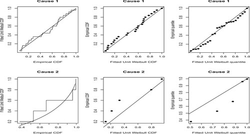
Figure 2. Plotting of profile likelihood of Unit Weibull distribution for Data I.

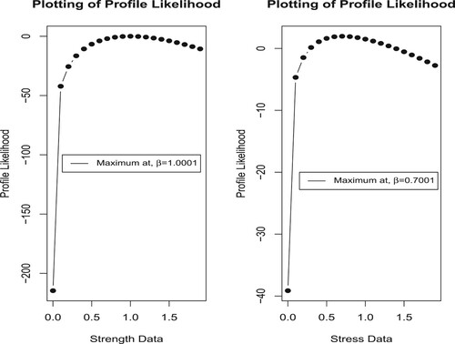
Table 9. Test of goodness results for Data I.

	Data Z				Data T
Distribution	${\hat{\theta }}_1$	$\widehat{\text{β}}$	kolm	prob	${\hat{\theta }}_2$	$\widehat{\text{β}}$	kolm	prob
Unit Weibull	1.036154	0.996209	0.10942	0.8941	2.114108	0.7038222	0.27094	0.7744
Log-Lindley	1.35382	1.657287	0.12827	0.7586	2.818937	1.870696	0.30465	0.6457
Kumaraswamy	0.9796485	0.9180274	0.097555	0.9526	1303.455	267962.3	0.8	0.00064
Unit Gamma	1.034798	1531143	0.11054	0.8874	2.431368	3596707	0.30245	0.6543

Table 10. Estimation results for Data I.

${\hat{\theta }}_1$	${\hat{\theta }}_2$	$\hat{\lambda }$	$R_{s,k}$	$R_{s,k}^{LS}$	$R_{s,k}^{WLS}$	$R_{s,k}^{MPS}$	$\widehat{R_{s,j}^L}$	$\widehat{R_{s,j}^{MH}}$	Boot-p	Boot-t	ACI	HPD
1.056552	2.366079	0.937018	0.6906617	0.7699177	0.7597839	0.5719439	0.8608635	0.5608937;	(0.3446559, 0.8383069)	(0.4110284, 0.8660306)	(0.4799626, 0.9013608)	(0.3660185, 0.7648702)

1. Further equivalence testing between UW stress and strength parameters ${\text{β}}_1$ and ${\text{β}}_2$ is performed. The likelihood ratio test is applied to derive the inference.

2. $H_0:{\text{β}}_1={\text{β}}_2$ versus $H_1:{\text{β}}_1\ne {\text{β}}_2$. The test statistic is $\mathrm{\Delta }=-2({\log }_0-{\log }_1)$ which is ${\chi }^2\left(1\right)$.

3. The estimates of corresponding log likelihoods under data I with $H_0:{\text{β}}_1={\text{β}}_2$ and alternative hypotheses $H_1:{\text{β}}_1\ne {\text{β}}_2$ are ${\log }_0=1.607646$ and ${\log }_1=1.979536$, respectively. Here, we obtain $\mathrm{\Delta }=0.7437795$ with probability value $0.388478$.

4. We see that null hypothesis ${\text{β}}_1={\text{β}}_2$ indicates favourable result under $5\mathrm{\%}$ significance. Thus we conclude that ${\text{β}}_1$ and ${\text{β}}_2$ may be equal for the considered numerical example.

Data Set II:

The second data set defines 12 core samples from petroleum reservoirs that were sampled by 4 cross-sections. There are a total of 48 observations in this study. Core samples are measured for permeability and each cross-section defined using following components: total area of pores, total perimeter of pores and shape. The data set is available in R language [40], especially on data.frame named rock. Table 11 contains associated estimates for all competing models. We see that UW distribution is a good representative model for the given data. We have also plotted P–P and Q–Q plots (Figure 3) of the data. We observe that data fitted satisfactorily by the UW model. In Figure 4, we plotted curve of the profile likelihood function. This is concave in nature, i.e. unimodal function with maximum at $\text{β}=5$ for strength data and $\text{β}=9$ for stress data. Following [41], we further explore histogram plot of bootstrap samples for the logit of $R_{s,k}$ based on 3000 replications, see Figure 5. The histogram resembles of a normal distribution with approximate mean 1.727348 and standard deviation 0.5171634. Further associated K–S estimate (0.029392) and P-value (0.06314) also indicate normality of bootstrap samples for the logit of $R_{s,k}$. In Table 12, estimates for the unknown reliability are evaluated for the complete data case. Associated intervals are also computed. We mention that Bayesian computations are performed against improper prior distribution.

Figure 3. PP–QQ plots of the unit Weibull distribution for Data II.

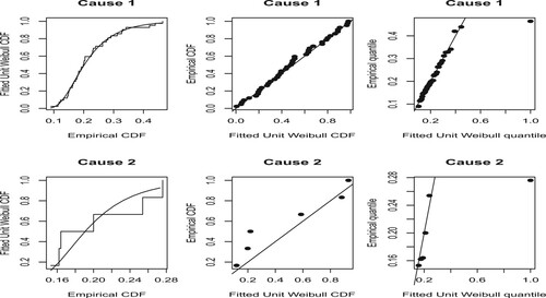
Figure 4. Plotting of profile likelihood of Unit Weibull distribution for Data II.

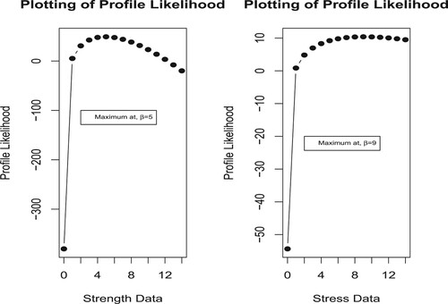
Figure 5. Plotting of logit $R_{s,k}$ of Unit Weibull distribution for Data II.

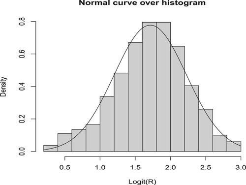
Table 11. Goodness of fit for Data II.

	Data Z				Data T
Distribution	${\hat{\theta }}_1$	$\widehat{\text{β}}$	kolm	prob	${\hat{\theta }}_2$	$\widehat{\text{β}}$	kolm	prob
Unit Weibull	0.0685	4.917	0.0836	0.9306	0.0073	9.006	0.2812	0.6361
Log-Lindley	70.89	0.6458	0.4220	6.36e−07	103.7524	0.6233	0.5462	0.0332
Kumaraswamy	38.98	2.647	0.152	0.2801	216.6	3.553	0.2403	0.8074
Unit Gamma	0.6323	1027753	0.4221	6.3e−07	0.6139	1114084	0.5463	0.0332

Table 12. Estimation results for Data II.

${\hat{\theta }}_1$	${\hat{\theta }}_2$	$\widehat{\text{β}}$	$R_{s,k}$	$R_{s,k}^{LS}$	$R_{s,k}^{WLS}$	$R_{s,k}^{MPS}$	$\widehat{R_{s,j}^L}$	$\widehat{R_{s,j}^{MH}}$	Boot-p	Boot-t	ACI	HPD
0.0588	0.0671	5.1585	0.8598	0.7792	0.7881	0.7338	0.8012	0.8741;	(0.6285, 0.9348)	(0.6192, 0.9534)	( 0.7567,0.9630)	( 0.7782, 0.9537)

We consider s = 1 and $k=7$ which is like 1-out-of-7: G system. Let $Y_1$ denote the 8th breaking stress and $X_{1k}$, $k=1,2,\dots ,7$, be the failure times of observations numbered 1 to 7. Further let $Y_2$ denote the 16th observation and $X_{2k}$ be the failure times from 9 to 15. We carry on this data processing up to 48th failure, then we get n = 6 data for Y. The obtained data $(X,Y)$ are as follows: $\begin{array}{rl}X& =\left[\begin{array}{ccccc}0.090& 0.149& 0.183& 0.117& 0.122\\ 0.204& 0.162& 0.151& 0.148& 0.229\\ 0.204& 0.263& 0.200& 0.145& 0.114\\ 0.281& 0.179& 0.192& 0.133& 0.225\\ 0.198& 0.327& 0.154& 0.276& 0.177\\ 0.329& 0.230& 0.464& 0.420& 0.201\end{array}\right.\\ & \left.\begin{array}{cc}0.167& 0.190\\ 0.232& 0.173\\ 0.291& 0.240\\ 0.341& 0.312\\ 0.439& 0.164\\ 0.263& 0.182\end{array}\right]\mathrm{a}\mathrm{n}\mathrm{d}Y=\left[\begin{array}{c}0.164\\ 0.153\\ 0.162\\ 0.276\\ 0.254\\ 0.200\end{array}\right].\end{array}$

1. Further equivalence testing between UW stress and strength parameters ${\text{β}}_1$ and ${\text{β}}_2$ is performed for the data set II. The likelihood ratio test is applied to derive the inference.

2. The estimates of corresponding log likelihoods under data II with $H_0:{\text{β}}_1={\text{β}}_2$ and alternative hypotheses $H_1:{\text{β}}_1\ne {\text{β}}_2$ are, ${\log }_0=58.38494$ and, ${\log }_1=59.55056$, respectively. Here, we obtain $\mathrm{\Delta }=2.331241$ with a probability value $0.126804$.

3. We see that null hypothesis ${\text{β}}_1={\text{β}}_2$ indicates favourable result under $5\mathrm{\%}$ significance. Thus we conclude that ${\text{β}}_1$ and ${\text{β}}_2$ may be equal for the considered numerical example.

6. Conclusion

We have investigated inference upon a stress–strength parameter for UW distribution. The four frequentist methods of estimation have been used to obtain the system reliability with known and unknown β. Besides, asymptotic and two bootstrap CIs are obtained. Further Bayes inferences of $R_{s,k}$ are studied against different approximation techniques. The Bayes credible interval is discussed utilizing posterior samples generated from an MCMC method. Besides, unbiased estimation of reliability is also evaluated for known β case. Our numerical results suggest that Bayes procedure yields better inference compared to MLE and UMVUE. It is also seen that asymptotic, bootstrap and Bayesian intervals exhibit relatively good CP behaviour. However, width of Bayes intervals remains narrower than the corresponding asymptotic and bootstrap CIs. We present two numerical examples to demonstrate and observe the reliability for one system configuration. We found that WLSE provides marginally better results than the corresponding LSE estimates. Further inference obtained from the MPS method shows good behaviour than the WLSE method. We further note that MLE also improves LSE and WLSE. However, MLE and MPS methods are incomparable as in some case MLE performs better than MPS and in other case opposite behaviour is observed. We observe that if proper prior is available then Bayesian procedures have an advantage over the other methods. Overall, better inference of this particular parametric function can be derived under known β case. Although inference is studied when stress–strength components have the UW distributions, however, such studies can be conducted under assumption stress–strength components have different distributions. Moreover, estimation for the multicomponent stress–strength reliability for system with dependent components seems also of interest and importance in practice, which will be studied in the future. In near future, we also try to study such problems under some censoring schemes.

Acknowledgements

Authors thank the reviewer and Editor for their useful comments to improve our manuscript. This work was funded by Deanship of Scientific Research at Princess Nourah bint Abdulrahman University, through the Program of Research Project(Grant No. 41-PRFA-P-14).

Disclosure statement

No potential conflict of interest was reported by the authors.

Additional information

Funding

This work was supported by Deanship of Scientific Research at Princess Nourah bint Abdulrahman University [41-PRFA-P-14].

References

- Mudholkar GS, Srivastava DK. Exponentiated Weibull family for analyzing bathtub failure-rate data. IEEE Trans Reliab. 1993;42:299–302.
- Mudholkar GS, Srivastava DK, Freimer M. The exponentiated Weibull family: a reanalysis of the bus-motor-failure data. Technometrics. 1995;37:436–445.
- Singh U, Gupta PK, Upadhyay SK. Estimation of parameters for exponentiated-Weibull family under type-II censoring scheme. Comput Statist Data Anal. 2005;48:509–523.
- Marshall AW, Olkin I. A new method for adding a parameter to a family of distributions with application to the exponential and Weibull families. Biometrika. 1997;84:641–652.
- Zhang T, Xie M. Failure data analysis with extended Weibull distribution. Comm Statist Simul Comput. 2007;36:579–592.
- Jiang H, Xie M, Tang LC. Markov chain Monte Carlo methods for parameter estimation of the modified Weibull distribution. J Appl Stat. 2008;35:647–658.
- Lai CD, Xie M, Murthy DNP. A modified Weibull distribution. IEEE Trans Reliab. 2003;52:33–37.
- Ng HKT. Parameter estimation for a modified Weibull distribution, for progressively type-II censored samples. IEEE Trans Reliab. 2005;54:374–380.
- Cooray K. Generalization of the Weibull distribution: the odd Weibull family. Stat Model. 2006;6:265–277.
- Alzaatreh A, Famoye F, Lee C. A new method for generating families of continuous distributions. METRON. 2013;71(1):63–79.
- Bourguignon M, Silva RB, Cordeiro GM. The Weibull-G family of probability distributions. J Data Sci. 2014;11:1–27.
- Korkmaz MC. A new family of the continuous distributions: the extended Weibull-G family. Commun Fac Sci Univ Ank Ser A1 Math Stat. 2019;68(1):248–270.
- Kumaraswamy P. A generalized probability density function for double-bounded random processes. J Hydrol (Amst). 1980;46(1–2):79–88.
- Mazucheli J, Menezes AFB, Dey S. Improved maximum-likelihood estimators for the parameters of the unit-gamma distribution. Commun Statist Theory Methods. 2018a;47(15):3767–3778.
- Mazucheli J, Menezes AFB, Dey S. The unit-Birnbaum–Saunders distribution with applications. Chil J Stat. 2018b;9(1):47–57.
- Mazucheli J, Menezes AFB, Dey S. Unit-Gompertz distribution with applications. Statistica. 2019;79(1):25–43.
- Mazucheli J, Menezes AFB, Ghitany ME. The unit-Weibull distribution and associated inference. J Appl Probab Stat. 2018;13(2):1–22.
- Bhattacharyya G, Johnson RA. Estimation of reliability in a multicomponent stress–strength model. J Am Stat Assoc. 1974;69(348):966–970.
- Rao GS, Aslam M, Kundu D. Burr-XII distribution parametric estimation and estimation of reliability of multicomponent stress–strength. Commun Statist Theory Methods. 2015;44:4953–4961.
- Dey S, Mazucheli J, Anis M. Estimation of reliability of multicomponent stress–strength for a Kumaraswamy distribution. Commun Statist Theory Methods. 2017;46:1560–1572.
- Kayal T, Tripathi YM, Dey S, et al. On estimating the reliability in a multicomponent stress–strength model based on Chen distribution. Commun Statist Theory Methods. 2020;49(10):2429–2447.
- Kizilaslan F, Nadar M. Classical and Bayesian estimation of reliability in multicomponent stress–strength model based on Weibull distribution. Rev Colomb Estadstica. 2015;38(2):67–484.
- Pak A, Gupta AK, Khoolenjani NB. On reliability in a multicomponent stress–strength model with power Lindley distribution. Rev Colomb Estadstica. 2018;41(2):251–267.
- Dey S, Moala FA. Estimation of reliability of multicomponent stress–strength of a bathtub shape or increasing failure rate function. Int J Qual Reliab Manag. 2019;36(2):122–136.
- Seadawy AR, Luc D, Yue C. Travelling wave solutions of the generalized nonlinear fifth-order KdV water wave equations and its stability. J Taibah Univ Sci. 2017;11:623–633.
- Seadawy AR, Iqbal M, Luc D. Nonlinear wave solutions of the Kudryashov–Sinelshchikov dynamical equation in mixtures liquid–gas bubbles under the consideration of heat transfer and viscosity. J Taibah Univ Sci. 2019;13:1060–1072.
- Ahmad H, Seadawy AR, Khan TA, et al. Analytic approximate solutions for some nonlinear parabolic dynamical wave equations. J Taibah Univ Sci. 2020;14:346–358.
- Khaliq Q, Riaz M, Ahmad S. On designing a new Tukey-EWMA control chart for process monitoring. Int J Adv Manufacturing Technol. 2016;82(1–4):1–23.
- Abbasi SA, Khaliq QUA, Omar MH, et al. On designing a sequential based EWMA structure for efficient process monitoring. J Taibah Univ Sci. 2020;14(1):177–191.
- Efron B. The jackknife, the bootstrap, and other resampling plans. Philadelphia (PA): SIAM; 1982.
- Hall P. On some simple estimates of an exponent of regular variation. J R Statist Soc Ser B (Method). 1982;44(1):37–42.
- Swain JJ, Venkatraman S, Wilson JR. Least-squares estimation of distribution functions in Johnson's translation system. J Stat Comput Simul. 1988;29(4):271–297.
- Cheng R, Amin N. Estimating parameters in continuous univariate distributions with a shifted origin. J R Statist Soc Ser B (Method). 1983;45(3):394–403.
- Lindley DV. Approximate bayesian methods. Trabajos Estadst Invest Oper. 1980;31(1):223–245.
- Hastings WK. Monte Carlo sampling methods using Markov chains and their applications. Biometrika. 1970;57(1):97–109.
- Metropolis N, Rosenbluth AW, Rosenbluth MN, et al. Equation of state calculations by fast computing machines. J Chem Phys. 1953;21(6):1087–1092.
- Chen M-H, Shao Q-M. Monte Carlo estimation of Bayesian credible and HPD intervals. J Comput Graph Stat. 1999;8(1):69–92.
- Basirat M, Baratpour S, Ahmadi J. Statistical inferences for stress–strength in the proportional hazard models based on progressive type-II censored samples. J Stat Comput Simul. 2015;85(3):431–449.
- Xia Z, Yu J, Cheng L, et al. Study on the breaking strength of jute fibres using modified Weibull distribution. Comp Part A Appl Sci Manufac. 2009;40(1):54–59.
- Team RC. R: a language and environment for statistical computing. 2013.
- Al-Mutairi DK, Ghitany ME, Kundu D. Inferences on stress–strength reliability from Lindley distributions. Commun Statist Theory Methods. 2013;42(8):1443–1463.