New exact and numerical solutions with their stability for Ito integro-differential equation via Riccati–Bernoulli sub-ODE method

Abstract

This paper points out several exact travelling wave solutions for $(1+1)$-dimensional Ito integro-differential equation via the Riccati–Bernoulli sub-ODE approach. We also aim to develop a numerical solution of the respective equation using central finite difference formulas. The stability of the presented exact and numerical solutions is also deduced using the Hamiltonian system and Von Neumann's concept, respectively. Moreover, the numerical schemes are studied in terms of their accuracy. The relative error arising from executing the numerical method is exhibited. We compare our results with others published in some articles. The accomplished numerical solutions are successfully compared with the analytical ones. The used processes can be extended to solve more integrable problems as well as non-integrable ones.

Keywords:

• Ito equation
• Riccati–Bernoulli sub-ODE technique
• travelling wave solution
• numerical solution
• stability
• accuracy

AMS Subject Classifications:

• 65N06
• 65N40
• 65N45
• 65N50

1. Introduction

Most natural events are modelled and analysed using partial differential equations (PDEs). Nonlinear evolution equations usually contribute in giving efficient, acceptable and practical results when they are used to describe some phenomena. Therefore, such equations are commonly utilized to deal with some sophisticated problems arising in various fields such as biology, chemistry, fluid dynamics, fibres, condensed matter physics, heat transfer, plasma physics, optics, etc. Many experts have established a considerable number of techniques to discover and construct the exact solutions of the developed model. Among the existing ones, we reveal the following: the Adomian decomposition process [1,2], the sine-cosine principal [3,4], the rank analysis approach [5], the tanh–sech principal [6,7], the extended tanh process [8,9], the complex hyperbolic function concept [10,11], the $exp(-f(\zeta ))$-expansion approach [12,13]. For more methods, one can see [14–23].

Ito established a $(1+1)$-dimensional Ito equation in 1980. This equation is a generalization of the bilinear KdV problem [24]. The $(1+1)$-dimensional Ito equation reads as follows: (1) $\begin{array}{r}{U}_{tt}+U_{xxxt}+3(2U_x{U}_t+U{U}_{xt})+3U_{xx}{\int }_{-\mathrm{\infty }}^x{U}_t\mathrm{d}\zeta =0.\end{array}$(1) According to [25], Equation (1(1) $\begin{array}{r}{U}_{tt}+U_{xxxt}+3(2U_x{U}_t+U{U}_{xt})+3U_{xx}{\int }_{-\mathrm{\infty }}^x{U}_t\mathrm{d}\zeta =0.\end{array}$(1) ) is primarily related to the Fokker–Planck model. Ito equation has received much attention from several researchers. For instance, the authors in [26] have extracted the exact solutions of Equation (1(1) $\begin{array}{r}{U}_{tt}+U_{xxxt}+3(2U_x{U}_t+U{U}_{xt})+3U_{xx}{\int }_{-\mathrm{\infty }}^x{U}_t\mathrm{d}\zeta =0.\end{array}$(1) ) using three different techniques, namely, the generalized direct algebraic approach, the long simple equation process, and the modified F-expansion technique. In [25], the authors have applied the extended homoclinic test approach to construct some exact soliton solutions, including two soliton solutions, breather type of soliton, and periodic type of soliton. Moreover, the Kudryashov method is employed in [27] to obtain the exact solution of the $(1+1)$-dimensional form of the generalized Ito integro-differential equation.

Since our understanding of building exact travelling wave solutions for Ito equation is extensively based on minimal techniques, we employ the Riccati–Bernoulli sub-ODE method on the governing equation to discover some exact travelling wave solutions in the form of trigonometric and hyperbolic functions. The proposed technique, which allows us to achieve complicated algebraic calculations, is used to construct peaked wave solutions, solitary wave solutions, and exact wave solutions for nonlinear evolution equations [28]. Once the Riccati–Bernoulli equation approach is used, the proposed equation is changed to be a system of algebraic equations that can be easily solved. The central finite difference methods are also invoked to seek numerical results. Verily, the achieved results effectively contribute to explain some practically physical models and some complex problems.

2. Summary of the Riccati–Bernoulli sub-ODE process

This section is mainly devoted to briefly summarize the Riccati–Bernoulli Sub-ODE approach, as presented in [28]. Consider the following NPDE: (2) $\begin{array}{r}G(S,S_t,S_x,S_{tt},S_{xx},\dots )=0,\end{array}$(2) where x and t are independent variables. $S(x,t)$ plays the role of the solution of Equation (2(2) $\begin{array}{r}G(S,S_t,S_x,S_{tt},S_{xx},\dots )=0,\end{array}$(2) ).

• Substitute the transformation (3) $\begin{array}{r}S(x,t)=\psi (\eta ),\eta =kx-wt,\end{array}$(3) into Equation (2(2) $\begin{array}{r}G(S,S_t,S_x,S_{tt},S_{xx},\dots )=0,\end{array}$(2) ) to yield (4) $\begin{array}{r}Q(\psi ,{\psi }^{\prime },{\psi }^{″},{\psi }^{‴},\dots )=0,\end{array}$(4) where ψ is a solution for Equation (4(4) $\begin{array}{r}Q(\psi ,{\psi }^{\prime },{\psi }^{″},{\psi }^{‴},\dots )=0,\end{array}$(4) ). The first derivative of ψ is given by (5) $\begin{array}{r}{\psi }^{\prime }=a_0{\psi }^{2-n}+a_1\psi +a_2{\psi }^n.\end{array}$(5) Here, n is a user-specified integer. The parameters $a_0,a_1,$ and $a_2$ are obtained later.

• The second and third derivatives of Equation (5(5) $\begin{array}{r}{\psi }^{\prime }=a_0{\psi }^{2-n}+a_1\psi +a_2{\psi }^n.\end{array}$(5) ) with respect to η are given by (6) $\begin{array}{rl}{\psi }^{″}& ={\psi }^{-2n-1}(a_0{\psi }^2+a_1{\psi }^{n+1}+a_2{\psi }^{2n})\\ & (-a_0(n-2){\psi }^2+a_1{\psi }^{n+1}+a_{2}n{\psi }^{2n}),\end{array}$(6) (7) $\begin{array}{rl}{\displaystyle {\psi }^{‴}}& ={\psi }^{-3n-2}(a_0{\psi }^2+a_1{\psi }^{n+1}+a_2{\psi }^{2n})(a_0^2\\ & (2n^2-7n+6){\psi }^4+(2a_0{a}_2+a_1^2){\psi }^{2n+2}\\ & +a_0{a}_1(n^2-5n+6){\psi }^{n+3}+a_1{a}_{2}n(n+1)\\ & {\psi }^{3n+1}+a_2^{2}n(2n-1){\psi }^{4n}).\end{array}$(7)

• Here, we present some forms for the travelling wave solutions of Equation (4(4) $\begin{array}{r}Q(\psi ,{\psi }^{\prime },{\psi }^{″},{\psi }^{‴},\dots )=0,\end{array}$(4) ) depending on the value of n and the obtained parameters.

  1. If $n=1,$ then the travelling wave solution reads (8) $\begin{array}{r}\psi (\eta )={\mu }_0\exp \left(\sum _{i=0}^2{a}_i\eta \right).\end{array}$(8)

  2. If $n\ne 1,$ $a_1=0$ and $a_2=0,$ then the travelling wave solution is given by (9) $\begin{array}{r}\psi (\eta )=\sqrt[n-1]{a_0(n-1)(\eta +{\mu }_0)}.\end{array}$(9)

  3. If $n\ne 1,$ $a_1\ne 0$ and $a_2=0,$ then the travelling wave solution is expressed as (10) $\begin{array}{r}\psi (\eta )=\sqrt[n-1]{{\mu }_0\exp (a_1(n-1)\eta )-\frac{a_0}{a_1}}.\end{array}$(10)

  4. If $n\ne 1,$ $a_0\ne 0$ and $a_1^2-4a_0{a}_2<0,$ then the travelling wave solutions are shown as

     (11) $\begin{array}{rl}& \psi (\eta )\\ & {\displaystyle =\sqrt[1-n]{\begin{array}{c}\frac{\sqrt{4a_0{a}_2-a_1^2}}{2a_0}\\ {\displaystyle \times \tan (\frac{1}{2}(1-n)\sqrt{4a_0{a}_2-a_1^2}(\eta +{\mu }_0))}\\ {\displaystyle -\frac{a_1}{2a_0}}\end{array}}}\end{array}$(11) and

     (12) $\begin{array}{rl}& \psi (\eta )\\ & {\displaystyle =\sqrt[1-n]{\begin{array}{c}-\frac{\sqrt{4a_0{a}_2-a_1^2}}{2a_0}\\ {\displaystyle \cot (\frac{1}{2}(1-n)\sqrt{4a_0{a}_2-a_1^2}(\eta +{\mu }_0))}\\ {\displaystyle -\frac{a_1}{2a_0}}\end{array}}.}\end{array}$(12)

  5. If $n\ne 1,$ $a_0\ne 0$ and $a_1^2-4a_0{a}_2>0,$ then the travelling wave solutions are given by

     (13) $\begin{array}{rl}& \psi (\eta )\\ & {\displaystyle =\sqrt[1-n]{\begin{array}{c}-\frac{\sqrt{a_1^2-4a_0{a}_2}}{2a_0}\\ {\displaystyle \times \coth (\frac{1}{2}(1-n)\sqrt{a_1^2-4a_0{a}_2}(\eta +{\mu }_0))}\\ {\displaystyle -\frac{a_1}{2a_0}}\end{array}}}\end{array}$(13) and

     (14) $\begin{array}{rl}& {\displaystyle \psi (\eta )}\\ & {\displaystyle =\sqrt[1-n]{\begin{array}{c}-\frac{\sqrt{a_1^2-4a_0{a}_2}}{2a_0}\\ {\displaystyle \times \tanh (\frac{1}{2}(1-n)\sqrt{a_1^2-4a_0{a}_2}(\eta +{\mu }_0))}\\ {\displaystyle -\frac{a_1}{2a_0}}\end{array}}.}\end{array}$(14)

  6. If $n\ne 1,$ $a_0\ne 0$ and $a_1^2-4a_0{a}_2=0,$ we have (15) $\begin{array}{r}\psi (\eta )=\sqrt[1-n]{\frac{1}{a_0(n-1)(\eta +{\mu }_0)}-\frac{a_1}{2a_0}},\end{array}$(15) where ${\mu }_0$ is an arbitrary constant.

3. Travelling wave solution

This section concentrates on constructing some exact travelling wave solutions for $(1+1)$-dimensional form of the generalized Ito integro-differential equation given by (16) $\begin{array}{r}{U}_{tt}+U_{xxxt}+\alpha (2U_x{U}_t+U{U}_{xt})+\alpha U_{xx}{\int }_{-\mathrm{\infty }}^x{U}_t\mathrm{d}\zeta =0.\end{array}$(16) Here, α is a user-specified parameter. Equation (16(16) $\begin{array}{r}{U}_{tt}+U_{xxxt}+\alpha (2U_x{U}_t+U{U}_{xt})+\alpha U_{xx}{\int }_{-\mathrm{\infty }}^x{U}_t\mathrm{d}\zeta =0.\end{array}$(16) ) is firstly simplified by assuming that $U={\mathrm{\Phi }}_x$. Thus, Equation (16(16) $\begin{array}{r}{U}_{tt}+U_{xxxt}+\alpha (2U_x{U}_t+U{U}_{xt})+\alpha U_{xx}{\int }_{-\mathrm{\infty }}^x{U}_t\mathrm{d}\zeta =0.\end{array}$(16) ) becomes (17) $\begin{array}{r}{\mathrm{\Phi }}_{xtt}+{\mathrm{\Phi }}_{xxxxt}+\alpha ({\mathrm{\Phi }}_x{\mathrm{\Phi }}_t{)}_{xx}=0,\end{array}$(17) where x and t are the spatial and time variables, respectively. Substituting the transform (18) $\begin{array}{r}\mathrm{\Phi }(x,t)=\psi (\eta ),\eta =kx-wt,\end{array}$(18) into Equation (17(17) $\begin{array}{r}{\mathrm{\Phi }}_{xtt}+{\mathrm{\Phi }}_{xxxxt}+\alpha ({\mathrm{\Phi }}_x{\mathrm{\Phi }}_t{)}_{xx}=0,\end{array}$(17) ) and integrating twice w.r.t. η and taking the integration constants by zero yield (19) $\begin{array}{r}w{\psi }^{\prime }-k^3{\psi }^{‴}-\alpha k^2({\psi }^{\prime }{)}^2=0.\end{array}$(19) Here, k is a real number and w indicates the wave speed. Plugging Equation (5(5) $\begin{array}{r}{\psi }^{\prime }=a_0{\psi }^{2-n}+a_1\psi +a_2{\psi }^n.\end{array}$(5) ) and Equation (7(7) $\begin{array}{rl}{\displaystyle {\psi }^{‴}}& ={\psi }^{-3n-2}(a_0{\psi }^2+a_1{\psi }^{n+1}+a_2{\psi }^{2n})(a_0^2\\ & (2n^2-7n+6){\psi }^4+(2a_0{a}_2+a_1^2){\psi }^{2n+2}\\ & +a_0{a}_1(n^2-5n+6){\psi }^{n+3}+a_1{a}_{2}n(n+1)\\ & {\psi }^{3n+1}+a_2^{2}n(2n-1){\psi }^{4n}).\end{array}$(7) ) into Equation (19(19) $\begin{array}{r}w{\psi }^{\prime }-k^3{\psi }^{‴}-\alpha k^2({\psi }^{\prime }{)}^2=0.\end{array}$(19) ) and taking n = 0 give (20) $\begin{array}{rl}& -(a_0{\psi }^2+a_1\psi +a_2)[a_1{k}^2\psi (6a_{0}k+\alpha )+a_2{k}^2\\ & \times (2a_{0}k+\alpha )+a_0{k}^2{\psi }^2(6a_{0}k+\alpha )+a_1^2{k}^3-w]=0.\end{array}$(20) Equating the coefficients of ${\psi }^m$ to zero and solving the obtained algebraic system lead to (21) $\begin{array}{r}\begin{array}{rl}& \mathrm{Case}1:a_0=-\frac{\alpha }{6k},a_1=0,a_2=\frac{3w}{2\alpha k^2},\\ & \mathrm{Case}2:a_0=-\frac{\alpha }{6k},a_1=\pm \sqrt{\frac{w}{k^3}},a_2=0.\end{array}\end{array}$(21) In both cases, we observe that $a_1^2-4a_0{a}_2=\frac{w}{k^3}$. It is worth noting that $U_{i,j}$ and ${\mathrm{\Phi }}_{i,j}$ are the exact solutions of Equation (16(16) $\begin{array}{r}{U}_{tt}+U_{xxxt}+\alpha (2U_x{U}_t+U{U}_{xt})+\alpha U_{xx}{\int }_{-\mathrm{\infty }}^x{U}_t\mathrm{d}\zeta =0.\end{array}$(16) ) and Equation (17(17) $\begin{array}{r}{\mathrm{\Phi }}_{xtt}+{\mathrm{\Phi }}_{xxxxt}+\alpha ({\mathrm{\Phi }}_x{\mathrm{\Phi }}_t{)}_{xx}=0,\end{array}$(17) ), respectively. The index i indicates the solution number while j shows the case number. Hence, the exact solutions of Equation (17(17) $\begin{array}{r}{\mathrm{\Phi }}_{xtt}+{\mathrm{\Phi }}_{xxxxt}+\alpha ({\mathrm{\Phi }}_x{\mathrm{\Phi }}_t{)}_{xx}=0,\end{array}$(17) ) and Equation (16(16) $\begin{array}{r}{U}_{tt}+U_{xxxt}+\alpha (2U_x{U}_t+U{U}_{xt})+\alpha U_{xx}{\int }_{-\mathrm{\infty }}^x{U}_t\mathrm{d}\zeta =0.\end{array}$(16) ) can be formed as follows.

1. If $n\ne 1,$ $a_1\ne 0$ and $a_2=0$. Then, the solution of Equation (17(17) $\begin{array}{r}{\mathrm{\Phi }}_{xtt}+{\mathrm{\Phi }}_{xxxxt}+\alpha ({\mathrm{\Phi }}_x{\mathrm{\Phi }}_t{)}_{xx}=0,\end{array}$(17) ) under the values of the second case is given by (22) $\begin{array}{rl}& {\mathrm{\Phi }}_{1,2}(x,t)\\ & ={({\mu }_0\exp \left(\pm \sqrt{\frac{w}{k^3}}(kx+{\mu }_0-wt)\right)-\frac{\alpha \sqrt{k}}{6\sqrt{w}})}^{-1}.\end{array}$(22) Hence, the exact solution of Equation (16(16) $\begin{array}{r}{U}_{tt}+U_{xxxt}+\alpha (2U_x{U}_t+U{U}_{xt})+\alpha U_{xx}{\int }_{-\mathrm{\infty }}^x{U}_t\mathrm{d}\zeta =0.\end{array}$(16) ), which we obtain by taking the first derivative for ${\mathrm{\Phi }}_{1,2}$ with respect to x, is (23) $\begin{array}{rl}& U_{1,2}(x,t)\\ & =-\frac{k{\mu }_0\pm \sqrt{\frac{w}{k^3}}\exp (\pm \sqrt{\frac{w}{k^3}}(kx+{\mu }_0-tw))}{({\mu }_0\exp (\pm \sqrt{\frac{w}{k^3}}(kx+{\mu }_0-tw))-\frac{1}{6}\alpha \sqrt{\frac{k}{w}}{)}^2}.\end{array}$(23)

2. If $n\ne 1,$ $a_0\ne 0$ and $\frac{w}{k}<0$. Then, the solutions are given by

   In case 1: (24) $\begin{array}{r}{\mathrm{\Phi }}_{2,1}(x,t)=\frac{3k}{\alpha }\sqrt{\frac{w}{k^3}}\tan (\frac{1}{2}\sqrt{\frac{w}{k^3}}(kx-wt+{\mu }_0))\end{array}$(24) and (25) $\begin{array}{r}{\mathrm{\Phi }}_{3,1}(x,t)=-\frac{3k}{\alpha }\sqrt{\frac{w}{k^3}}\cot (\frac{1}{2}\sqrt{\frac{w}{k^3}}(kx-wt+{\mu }_0)).\end{array}$(25) In case 2: (26) $\begin{array}{rl}{\mathrm{\Phi }}_{4,2}(x,t)& =\frac{3k}{\alpha }\sqrt{\frac{w}{k^3}}\tan (\frac{1}{2}\sqrt{\frac{w}{k^3}}(kx-wt+{\mu }_0))\\ & -\frac{3}{\alpha }\sqrt{\frac{w}{k}}\end{array}$(26) and (27) $\begin{array}{rl}{\mathrm{\Phi }}_{5,2}(x,t)& =-\frac{3k}{\alpha }\sqrt{\frac{w}{k^3}}\cot (\frac{1}{2}\sqrt{\frac{w}{k^3}}(kx-wt+{\mu }_0))\\ & -\frac{3}{\alpha }\sqrt{\frac{w}{k}}.\end{array}$(27) Thus, the exact solutions of Equation (16(16) $\begin{array}{r}{U}_{tt}+U_{xxxt}+\alpha (2U_x{U}_t+U{U}_{xt})+\alpha U_{xx}{\int }_{-\mathrm{\infty }}^x{U}_t\mathrm{d}\zeta =0.\end{array}$(16) ), in both cases j = 1 and 2, are expressed as (28) $\begin{array}{r}{U}_{2,j}(x,t)=\frac{1.5w}{\alpha k}se{c}^2(0.5\sqrt{\frac{w}{k^3}}(kx+{\mu }_0-tw))\end{array}$(28) and (29) $\begin{array}{r}{U}_{3,j}(x,t)=\frac{1.5w}{\alpha k}cs{c}^2(0.5\sqrt{\frac{w}{k^3}}(kx+{\mu }_0-tw)).\end{array}$(29)

3. If $n\ne 1,$ $a_0\ne 0$ and $\frac{w}{k}>0$. Then, the solutions are shown as

   In case 1: (30) $\begin{array}{rl}{\mathrm{\Phi }}_{6,1}(x,t)& =-\frac{3k}{\alpha }\sqrt{\frac{w}{k^3}}\tanh (\frac{1}{2}\sqrt{\frac{w}{k^3}}(kx-wt+{\mu }_0))\end{array}$(30) and (31) $\begin{array}{rl}& {\mathrm{\Phi }}_{7,1}(x,t)=-\frac{3k}{\alpha }\sqrt{\frac{w}{k^3}}\\ & \coth (\frac{1}{2}\sqrt{\frac{w}{k^3}}(kx-wt+{\mu }_0)).\end{array}$(31) In case 2: (32) $\begin{array}{rl}& {\mathrm{\Phi }}_{8,2}(x,t)\\ & =-\frac{3k}{\alpha }\sqrt{\frac{w}{k^3}}\tanh (\frac{1}{2}\sqrt{\frac{w}{k^3}}(kx-wt+{\mu }_0))\\ & -\frac{3}{\alpha }\sqrt{\frac{w}{k}}\end{array}$(32) and (33) $\begin{array}{rl}{\mathrm{\Phi }}_{9,2}(x,t)& =-\frac{3k}{\alpha }\sqrt{\frac{w}{k^3}}\\ & \coth (\frac{1}{2}\sqrt{\frac{w}{k^3}}(kx-wt+{\mu }_0))\\ & -\frac{3}{\alpha }\sqrt{\frac{w}{k}},\end{array}$(33) where ${\mu }_0$ is an arbitrary constant. As a result, the exact solutions of Equation (16(16) $\begin{array}{r}{U}_{tt}+U_{xxxt}+\alpha (2U_x{U}_t+U{U}_{xt})+\alpha U_{xx}{\int }_{-\mathrm{\infty }}^x{U}_t\mathrm{d}\zeta =0.\end{array}$(16) ), in both cases j = 1 and 2, are (34) $\begin{array}{r}{U}_{4,j}(x,t)=\frac{1.5w}{\alpha k}{\mathrm{sech}}^2(0.5\sqrt{\frac{w}{k^3}}(kx+{\mu }_0-tw))\end{array}$(34) and (35) $\begin{array}{r}{U}_{5,j}(x,t)=-\frac{1.5w}{\alpha k}{\mathrm{csch}}^2(0.5\sqrt{\frac{w}{k^3}}(kx+{\mu }_0-tw)).\end{array}$(35)

4. Hamiltonian system

Hamiltonian system [29,30] which is given by (36) $\begin{array}{r}\theta (w)=\frac{1}{2}{\int }_a^b{\mathrm{\Phi }}^2(\zeta )\mathrm{d}\zeta \end{array}$(36) is employed in this article to figure out the interval in which the achieved travelling wave solutions are stable. Here, w denotes the wave speed, θ plays the role of the momentum, $a,b$ are the endpoints of the specified domain, and $\mathrm{\Phi }(\zeta )$ is the relevant solution. The required condition for the stability is given by (37) $\begin{array}{r}\frac{\mathrm{\partial }\theta }{\mathrm{\partial }w}>0\mathrm{\forall }\zeta \in [a,b].\end{array}$(37)

4.1. Stability of the travelling wave solution

In this subsection, the Hamiltonian system is used to seek the stability of the obtained exact solutions of Equation (17(17) $\begin{array}{r}{\mathrm{\Phi }}_{xtt}+{\mathrm{\Phi }}_{xxxxt}+\alpha ({\mathrm{\Phi }}_x{\mathrm{\Phi }}_t{)}_{xx}=0,\end{array}$(17) ). Applying Equation (36(36) $\begin{array}{r}\theta (w)=\frac{1}{2}{\int }_a^b{\mathrm{\Phi }}^2(\zeta )\mathrm{d}\zeta \end{array}$(36) ) on Equation (17(17) $\begin{array}{r}{\mathrm{\Phi }}_{xtt}+{\mathrm{\Phi }}_{xxxxt}+\alpha ({\mathrm{\Phi }}_x{\mathrm{\Phi }}_t{)}_{xx}=0,\end{array}$(17) ) over the domain $[0,60]$ leads to (38) $\begin{array}{r}\theta (w)=\frac{1}{2}{\int }_0^{60}{\mathrm{\Phi }}^2(\zeta )\mathrm{d}\zeta .\end{array}$(38) Therefore, (39) $\begin{array}{r}\theta (w)=\frac{9w(60-\frac{2\tanh (30\sqrt{\frac{w}{k^3}})}{\sqrt{\frac{w}{k^3}}})}{2{\alpha }^{2}k}.\end{array}$(39) Differentiating Equation (39(39) $\begin{array}{r}\theta (w)=\frac{9w(60-\frac{2\tanh (30\sqrt{\frac{w}{k^3}})}{\sqrt{\frac{w}{k^3}}})}{2{\alpha }^{2}k}.\end{array}$(39) ) with respect to w which indicates wave speed yields (40) $\begin{array}{rl}& \frac{\mathrm{\partial }\theta }{\mathrm{\partial }w}=\frac{9(60-\frac{2\tanh (30\sqrt{\frac{w}{k^3}})}{\sqrt{\frac{w}{k^3}}})}{2{\alpha }^{2}k}\\ & +\frac{9w(\frac{\tanh (30\sqrt{\frac{w}{k^3}})}{k^3(\frac{w}{k^3}{)}^{3/2}}-\frac{30{\mathrm{sech}}^2(30\sqrt{\frac{w}{k^3}})}{w})}{2{\alpha }^{2}k}.\end{array}$(40) Selecting the parameter values as w = 3.0, k = 2.0, $\alpha =0.50,$ and ${\mu }_0=-18.0,$ gives (41) $\begin{array}{r}\frac{\mathrm{\partial }\theta }{\mathrm{\partial }w}=525.303>0.\end{array}$(41) Thus, the sufficient condition of the stability is satisfied. Consequently, the obtained travelling wave solutions are stable over the selected domain $[0,60]$ and with the selected parameter values $w=3.0,k=2.0,\alpha =0.50,{\mu }_0=-18.0,$ and $t=0\to 30$.

In the subsequent section, we consider the numerical solution of Equation (17(17) $\begin{array}{r}{\mathrm{\Phi }}_{xtt}+{\mathrm{\Phi }}_{xxxxt}+\alpha ({\mathrm{\Phi }}_x{\mathrm{\Phi }}_t{)}_{xx}=0,\end{array}$(17) ) by employing the finite differences. The spatial derivatives in Equation (17(17) $\begin{array}{r}{\mathrm{\Phi }}_{xtt}+{\mathrm{\Phi }}_{xxxxt}+\alpha ({\mathrm{\Phi }}_x{\mathrm{\Phi }}_t{)}_{xx}=0,\end{array}$(17) ) are semi-discretized using central finite difference formulas with second-order accurate. Temporal derivatives are kept continuous. Once we have the result, we will obtain the numerical solution of Equation (16(16) $\begin{array}{r}{U}_{tt}+U_{xxxt}+\alpha (2U_x{U}_t+U{U}_{xt})+\alpha U_{xx}{\int }_{-\mathrm{\infty }}^x{U}_t\mathrm{d}\zeta =0.\end{array}$(16) ) by using the second-order finite difference formulas of the spatial direction in Φ, where $U={\mathrm{\Phi }}_x$.

5. Numerical solution

The central finite differences are employed in this section to establish the numerical results of Equation (17(17) $\begin{array}{r}{\mathrm{\Phi }}_{xtt}+{\mathrm{\Phi }}_{xxxxt}+\alpha ({\mathrm{\Phi }}_x{\mathrm{\Phi }}_t{)}_{xx}=0,\end{array}$(17) ) over the computational domain $[x_L,x_R]$. Here, $x_L$ and $x_R$ indicate the endpoints of the domain. The numerical solution of Equation (16(16) $\begin{array}{r}{U}_{tt}+U_{xxxt}+\alpha (2U_x{U}_t+U{U}_{xt})+\alpha U_{xx}{\int }_{-\mathrm{\infty }}^x{U}_t\mathrm{d}\zeta =0.\end{array}$(16) ) is also manifested. The adaptive moving mesh, line and normal techniques [31–33] can be used to build the numerical results of the governing equation. In order to develop the numerical solution of Equation (17(17) $\begin{array}{r}{\mathrm{\Phi }}_{xtt}+{\mathrm{\Phi }}_{xxxxt}+\alpha ({\mathrm{\Phi }}_x{\mathrm{\Phi }}_t{)}_{xx}=0,\end{array}$(17) ), we convert Equation (17(17) $\begin{array}{r}{\mathrm{\Phi }}_{xtt}+{\mathrm{\Phi }}_{xxxxt}+\alpha ({\mathrm{\Phi }}_x{\mathrm{\Phi }}_t{)}_{xx}=0,\end{array}$(17) ) into a first-order differential system in time. We assume that ${\mathrm{\Phi }}_t=V_x$. Then, Equation (17(17) $\begin{array}{r}{\mathrm{\Phi }}_{xtt}+{\mathrm{\Phi }}_{xxxxt}+\alpha ({\mathrm{\Phi }}_x{\mathrm{\Phi }}_t{)}_{xx}=0,\end{array}$(17) ) becomes (42) $\begin{array}{r}{V}_{xxt}+V_{xxxxx}+\alpha (V_{xx}{V}_x{)}_{xx}=0.\end{array}$(42) Equation (42(42) $\begin{array}{r}{V}_{xxt}+V_{xxxxx}+\alpha (V_{xx}{V}_x{)}_{xx}=0.\end{array}$(42) ) can be converted into the following system: (43) $\begin{array}{r}\begin{array}{l}{\mathrm{\Phi }}_t-V_x=0,\\ V_t+V_{xxx}+\alpha (\mathrm{\Phi }{V}_x{)}_x-\alpha \mathrm{\Phi }{V}_{xx}=0.\end{array}\end{array}$(43) Here, x and t play the role of the spatial and time variables, respectively. To gain a much faster and more stable scheme, we modify the second equation of system (43(43) $\begin{array}{r}\begin{array}{l}{\mathrm{\Phi }}_t-V_x=0,\\ V_t+V_{xxx}+\alpha (\mathrm{\Phi }{V}_x{)}_x-\alpha \mathrm{\Phi }{V}_{xx}=0.\end{array}\end{array}$(43) ). The considered boundary conditions, which we can deduce from Figure 3(a), are given by (44) $\begin{array}{r}{\mathrm{\Phi }}_x=V_x=0,\mathrm{at}x=x_L,x_R,\end{array}$(44) where $x_L$ and $x_R$ are the boundaries of the computational domain. The boundary conditions (44(44) $\begin{array}{r}{\mathrm{\Phi }}_x=V_x=0,\mathrm{at}x=x_L,x_R,\end{array}$(44) ) lead us to have fictitious points that we use to obtain the spatial derivatives at the endpoints of the domain. We need to generate initial conditions for system (43(43) $\begin{array}{r}\begin{array}{l}{\mathrm{\Phi }}_t-V_x=0,\\ V_t+V_{xxx}+\alpha (\mathrm{\Phi }{V}_x{)}_x-\alpha \mathrm{\Phi }{V}_{xx}=0.\end{array}\end{array}$(43) ). Hence, we consider the function V which is given by (45) $\begin{array}{r}V(x,t)={\int }_{x_L}^x\frac{\mathrm{\partial }\mathrm{\Phi }(\xi ,t)}{\mathrm{\partial }t}\mathrm{d}\xi .\end{array}$(45) Achieving the above integral leads to (46) $\begin{array}{r}V(x,t)=-\frac{3w\sqrt{\frac{w}{k^3}}\tanh (\frac{1}{2}\sqrt{\frac{w}{k^3}}(kx+{\mu }_0-tw))}{\alpha }.\end{array}$(46) Therefore, the initial conditions are given by (47) $\begin{array}{r}\begin{array}{rl}& {\mathrm{\Phi }}_{6,1}(x,0)=-\frac{3k}{\alpha }\sqrt{\frac{w}{k^3}}\tanh (\frac{1}{2}\sqrt{\frac{w}{k^3}}(kx+{\mu }_0)),\\ & V(x,0)=-\frac{3w\sqrt{\frac{w}{k^3}}\tanh (\frac{1}{2}\sqrt{\frac{w}{k^3}}(kx+{\mu }_0))}{\alpha }.\end{array}\end{array}$(47) We begin with splitting the interval $[x_L,x_R]$ into subintervals so that (48) $\begin{array}{r}{x}_n=x_L+nh\mathrm{\forall }n=0,1,\dots ,N_x,\end{array}$(48) where h denotes the space increment. As a result, the numerical solutions at the mesh points are defined by ${\mathrm{\Phi }}_n$ and $V_n$. The spatial derivatives are semi-discretized while the temporal derivatives are kept continuous. Hence, the resulting scheme is shown as follows: (49) $\begin{array}{rl}& {\displaystyle {\mathrm{\Phi }}_t{|}_n-\frac{1}{2h}(V_{n+1}-V_{n-1})=0,}\\ & {\displaystyle V_t{|}_n+V_{xxx}{|}_n+\alpha (\mathrm{\Phi }{V}_x{)}_x{|}_n-\alpha }\\ & \frac{{\mathrm{\Phi }}_{n+1}+{\mathrm{\Phi }}_n}{2h^2}(V_{n+1}-2V_n+V_{n-1})=0,\end{array}$(49) where the discretization of $V_{xxx}{|}_n$ and $(\mathrm{\Phi }{V}_x{)}_x{|}_n$ is given by $\begin{array}{rl}{V}_{xxx}{|}_n& =\frac{1}{2h^3}(V_{n+2}-3V_{n+1}+3V_n-V_{n-1}),\\ (\mathrm{\Phi }{V}_x{)}_x{|}_n& =\frac{1}{2h^2}[({\mathrm{\Phi }}_{n+1}+{\mathrm{\Phi }}_n)(V_{n+1}-V_n)\\ & +({\mathrm{\Phi }}_{n-1}+{\mathrm{\Phi }}_n)(V_{n-1}-V_n)],\end{array}$ subject to the boundary conditions (50) $\begin{array}{r}{\mathrm{\Phi }}_t=V_t=0,\mathrm{at}x=x_L,x_R.\end{array}$(50) The initial conditions are given by evaluating Equation (47(47) $\begin{array}{r}\begin{array}{rl}& {\mathrm{\Phi }}_{6,1}(x,0)=-\frac{3k}{\alpha }\sqrt{\frac{w}{k^3}}\tanh (\frac{1}{2}\sqrt{\frac{w}{k^3}}(kx+{\mu }_0)),\\ & V(x,0)=-\frac{3w\sqrt{\frac{w}{k^3}}\tanh (\frac{1}{2}\sqrt{\frac{w}{k^3}}(kx+{\mu }_0))}{\alpha }.\end{array}\end{array}$(47) ) at t = 0. Here, $h=(x_L-x_R)/N_x$. It is worth mentioning that we invoke the method of lines which depends on a standard ODE solver in FORTRAN software, DASPK solver [34]. This solver applies a standard backward differentiation formulas to approximate time derivatives. DASPK uses an iterative numerical method and also uses LU factorization to approximate the Jacobian matrix of the linearized system. This leads to successful and powerful performance. To have a less bandwidth for the matrix which results from the performance of the method, we use a unique system numbering for the unknowns ${\mathrm{\Phi }}_1,V_1,{\mathrm{\Phi }}_2,V_2,\dots ,{\mathrm{\Phi }}_{N-1},V_{N-1},{\mathrm{\Phi }}_N$ and $V_N$.

5.1. Accuracy of the scheme

This subsection deals with the accuracy of the numerical scheme using Taylor expansion. The finite differences are used to develop the accuracy of the schemes. Plugging Taylor expansion into the numerical schemes and simplifying the results lead to the accuracy of the schemes which are $O(\mathrm{\Delta }{t}^2,h^2)$. Thus, the accuracy of the schemes are from the second-order in time and space.

5.2. Stability of the scheme

This subsection is assigned to test the stability of the obtained schemes using Von Neumann's concept. We first convert system (43(43) $\begin{array}{r}\begin{array}{l}{\mathrm{\Phi }}_t-V_x=0,\\ V_t+V_{xxx}+\alpha (\mathrm{\Phi }{V}_x{)}_x-\alpha \mathrm{\Phi }{V}_{xx}=0.\end{array}\end{array}$(43) ) to a linear system by taking $c_0={\mathrm{\Phi }}_x{|}_n^m$. Von Neumann's definition is given by (51) $\begin{array}{r}{\mathrm{\Phi }}_n^m={\gamma }_0^m\exp (\mathrm{i}h\eta n),V_n^m={\gamma }_1^m\exp (\mathrm{i}h\eta n),\end{array}$(51) where ${\gamma }_{0,1}$ and ξ are constants. Plugging Equations (51(51) $\begin{array}{r}{\mathrm{\Phi }}_n^m={\gamma }_0^m\exp (\mathrm{i}h\eta n),V_n^m={\gamma }_1^m\exp (\mathrm{i}h\eta n),\end{array}$(51) ) into Equations (49(49) $\begin{array}{rl}& {\displaystyle {\mathrm{\Phi }}_t{|}_n-\frac{1}{2h}(V_{n+1}-V_{n-1})=0,}\\ & {\displaystyle V_t{|}_n+V_{xxx}{|}_n+\alpha (\mathrm{\Phi }{V}_x{)}_x{|}_n-\alpha }\\ & \frac{{\mathrm{\Phi }}_{n+1}+{\mathrm{\Phi }}_n}{2h^2}(V_{n+1}-2V_n+V_{n-1})=0,\end{array}$(49) ) gives (52) $\begin{array}{r}\begin{array}{l}{r}_1{V}_n^{m+1}+0{\mathrm{\Phi }}_n^{m+1}=V_n^m,\\ r_2{V}_n^{m+1}+{\mathrm{\Phi }}_n^{m+1}={\mathrm{\Phi }}_n^m.\end{array}\end{array}$(52) Hence, system (52(52) $\begin{array}{r}\begin{array}{l}{r}_1{V}_n^{m+1}+0{\mathrm{\Phi }}_n^{m+1}=V_n^m,\\ r_2{V}_n^{m+1}+{\mathrm{\Phi }}_n^{m+1}={\mathrm{\Phi }}_n^m.\end{array}\end{array}$(52) ) can be easily expressed as follows: (53) $\begin{array}{r}\left[\begin{array}{cc}{r}_1& 0\\ r_2& 1\end{array}\right]{\left[\begin{array}{c}V\\ \mathrm{\Phi }\end{array}\right]}^{m+1}={\left[\begin{array}{c}V\\ \mathrm{\Phi }\end{array}\right]}^m.\end{array}$(53) Then, (54) $\begin{array}{r}{\left[\begin{array}{c}V\\ \mathrm{\Phi }\end{array}\right]}^{m+1}=A{\left[\begin{array}{c}V\\ \mathrm{\Phi }\end{array}\right]}^m,\end{array}$(54) where $A={\left[\begin{array}{cc}{r}_1& 0\\ r_2& 1\end{array}\right]}^{-1}.$ The values of $r_1$ and $r_2$ are $\begin{array}{rl}& r_1=1+\mathrm{i}\alpha c_0\tau \sin (h\xi )-2\frac{\tau }{h^2}{\sin }^2(h\xi /2)({\mathrm{e}}^{\mathrm{i}h\xi }-1),\\ & r_2=-\mathrm{i}\tau \sin (h\xi ),\end{array}$ where $c_0={\mathrm{\Phi }}_x{|}_n^m$, $\tau =\mathrm{\Delta }t/h,$ and $\mathrm{\Delta }t$ is the time increment. Note that Von Neumann's condition of the stability is that the maximum eigenvalue of A must be less than or equal one. Thus, the eigenvalues of the matrix A can be obtained using Maple or Mathematica software to have (55) $\begin{array}{r}{\lambda }_1=1,{\lambda }_2=\frac{1}{r_1}.\end{array}$(55) It can be simply observed that the maximum value of the eigenvalues is one. Consequently, the respective numerical scheme is unconditionally stable.

6. Comparison and discussion

Throughout this article, we have constructed novel and more general travelling wave solutions than the exact solutions obtained in various published papers such as those written in [27]. The Kudryashov method was used in [27] to present one rational exact solution based on the exponential function. However, we have utilized the Riccati–Bernoulli Sub-ODE process to construct several solitary wave solutions. The achieved solutions in this article are expressed in the form of trigonometric and hyperbolic functions. The Riccati–Bernoulli Sub-ODE technique is more effective than the Kudryashov method. Furthermore, the used numerical technique is reliable and effective.

The agreement between the analytical and numerical results is highly the same. As can be observed in Figure 5, both exact and numerical results coincide and are identical. Figure 6 exhibits the exact travelling wave solutions for $U(x,t)$ in Equation (16(16) $\begin{array}{r}{U}_{tt}+U_{xxxt}+\alpha (2U_x{U}_t+U{U}_{xt})+\alpha U_{xx}{\int }_{-\mathrm{\infty }}^x{U}_t\mathrm{d}\zeta =0.\end{array}$(16) ) and $\mathrm{\Phi }(x,t)$ in Equation (17(17) $\begin{array}{r}{\mathrm{\Phi }}_{xtt}+{\mathrm{\Phi }}_{xxxxt}+\alpha ({\mathrm{\Phi }}_x{\mathrm{\Phi }}_t{)}_{xx}=0,\end{array}$(17) ), which are almost the same as the numerical solutions presented in Figure 7 for the same equations. Figures 1, 4, 5, 6 and 7 are plotted under the value of the parameters $k=2,{\mu }_0=-18,\alpha =0.5,w=3$. Figure 2 is sketched under the parameter values $k=-10,{\mu }_0=15,\alpha =1,w=1,$ to satisfy the condition $\frac{w}{k}<0,$ while Figure 3 is depicted under the parameter values $k=2,{\mu }_0=15,\alpha =1,w=1,$ to satisfy the condition $\frac{w}{k}>0$.

Figure 1. (a) The exact solution $U_{1,2}$ of Equation (16(16) $\begin{array}{r}{U}_{tt}+U_{xxxt}+\alpha (2U_x{U}_t+U{U}_{xt})+\alpha U_{xx}{\int }_{-\mathrm{\infty }}^x{U}_t\mathrm{d}\zeta =0.\end{array}$(16) ). (b) The exact solution ${\mathrm{\Phi }}_{1,2}$ of Equation (17(17) $\begin{array}{r}{\mathrm{\Phi }}_{xtt}+{\mathrm{\Phi }}_{xxxxt}+\alpha ({\mathrm{\Phi }}_x{\mathrm{\Phi }}_t{)}_{xx}=0,\end{array}$(17) ). The used parameter values are $w=3.0,k=2.0,\alpha =0.50,{\mu }_0=-18.0,$ $t=0\to 30$ and $x=0\to 60$.

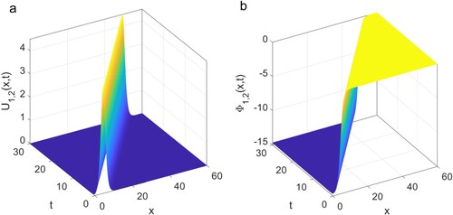
Figure 2. The exact solution $U_{2,j}$ of Equation (16(16) $\begin{array}{r}{U}_{tt}+U_{xxxt}+\alpha (2U_x{U}_t+U{U}_{xt})+\alpha U_{xx}{\int }_{-\mathrm{\infty }}^x{U}_t\mathrm{d}\zeta =0.\end{array}$(16) ). The used parameter values are $k=-10,{\mu }_0=+15,\alpha =1,w=1$.

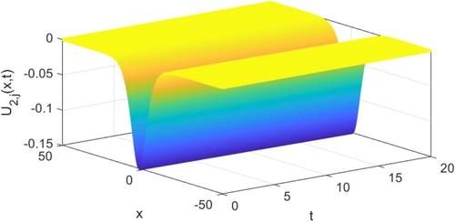
Figure 3. The graphs in (a) and (b) illustrate the time evolution of the exact solutions $U_{4,j}$ and $U_{5,j}$ of Equation (16(16) $\begin{array}{r}{U}_{tt}+U_{xxxt}+\alpha (2U_x{U}_t+U{U}_{xt})+\alpha U_{xx}{\int }_{-\mathrm{\infty }}^x{U}_t\mathrm{d}\zeta =0.\end{array}$(16) ), respectively. The used parameter values are $k=2,{\mu }_0=+15,\alpha =1,w=1$.

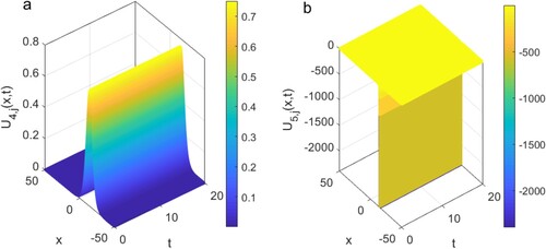
Figure 4. The graphs in (a) and (b) depict a 2D time evolution for the numerical solutions $U(x,t)$ of Equation (16(16) $\begin{array}{r}{U}_{tt}+U_{xxxt}+\alpha (2U_x{U}_t+U{U}_{xt})+\alpha U_{xx}{\int }_{-\mathrm{\infty }}^x{U}_t\mathrm{d}\zeta =0.\end{array}$(16) ) and $\mathrm{\Phi }(x,t)$ of Equation (17(17) $\begin{array}{r}{\mathrm{\Phi }}_{xtt}+{\mathrm{\Phi }}_{xxxxt}+\alpha ({\mathrm{\Phi }}_x{\mathrm{\Phi }}_t{)}_{xx}=0,\end{array}$(17) ), respectively. The parameter values are $w=3.0,k=2.0,\alpha =0.50,{\mu }_0=-18.0,$ $t=0\to 30$ and $x=0\to 60$.

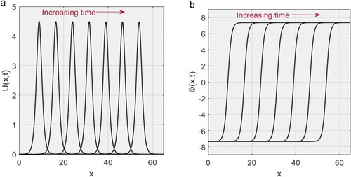
Figure 5. Presenting a precise comparison between the exact and numerical results of $U(x,t)$ in Equation (16(16) $\begin{array}{r}{U}_{tt}+U_{xxxt}+\alpha (2U_x{U}_t+U{U}_{xt})+\alpha U_{xx}{\int }_{-\mathrm{\infty }}^x{U}_t\mathrm{d}\zeta =0.\end{array}$(16) ) (a) and $\mathrm{\Phi }(x,t)$ in Equation (17(17) $\begin{array}{r}{\mathrm{\Phi }}_{xtt}+{\mathrm{\Phi }}_{xxxxt}+\alpha ({\mathrm{\Phi }}_x{\mathrm{\Phi }}_t{)}_{xx}=0,\end{array}$(17) ) (b). The blue-dashed lines present the exact solutions and the black-solid lines indicate the numerical results. The parameter values are $w=3.0,k=2.0,\alpha =0.50,{\mu }_0=-18.0,$ $t=0\to 30$ and $x=0\to 60$.

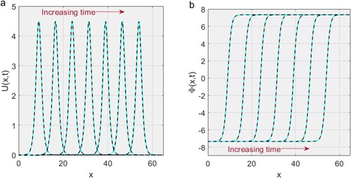
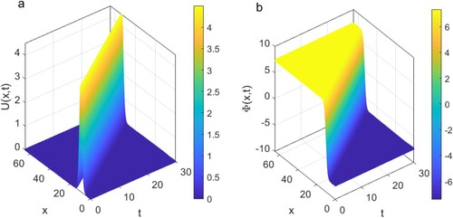
Figure 6. Presenting a 3D time evolution for the exact solutions U of Equation (16(16) $\begin{array}{r}{U}_{tt}+U_{xxxt}+\alpha (2U_x{U}_t+U{U}_{xt})+\alpha U_{xx}{\int }_{-\mathrm{\infty }}^x{U}_t\mathrm{d}\zeta =0.\end{array}$(16) ) and Φ of Equation (17(17) $\begin{array}{r}{\mathrm{\Phi }}_{xtt}+{\mathrm{\Phi }}_{xxxxt}+\alpha ({\mathrm{\Phi }}_x{\mathrm{\Phi }}_t{)}_{xx}=0,\end{array}$(17) ). The parameter values are $w=3.0,k=2.0,\alpha =0.50,{\mu }_0=-18.0,$ $t=0\to 30$ and $x=0\to 60$.

Figure 7. Illustrating a 3D time evolution for the numerical results U of Equation (16(16) $\begin{array}{r}{U}_{tt}+U_{xxxt}+\alpha (2U_x{U}_t+U{U}_{xt})+\alpha U_{xx}{\int }_{-\mathrm{\infty }}^x{U}_t\mathrm{d}\zeta =0.\end{array}$(16) ) and Φ of Equation (17(17) $\begin{array}{r}{\mathrm{\Phi }}_{xtt}+{\mathrm{\Phi }}_{xxxxt}+\alpha ({\mathrm{\Phi }}_x{\mathrm{\Phi }}_t{)}_{xx}=0,\end{array}$(17) ). The parameter values are $w=3.0,k=2.0,\alpha =0.50,{\mu }_0=-18.0,$ $t=0\to 30$ and $x=0\to 60$.

Regarding the stability, the Hamiltonian system shows that the travelling wave solution is stable over the selected domain $[0,60]$ with the parameter values $w=3.0,k=2.0,\alpha =0.50,{\mu }_0=-18.0,$ and $t=0\to 30$. We utilize Von Neumann's concept to testify the relevant numerical scheme's stability and we find that the scheme is unconditionally stable. Taylor expansion is used to examine the accuracy of the numerical scheme. We obtain that the accuracy is from second order in time and space. That is $O(\mathrm{\Delta }{t}^2,h^2)$. Further, Table 1 illustrates an essential tool for recognizing the validity of the applied numerical procedure. As can be easily observed, $L_2$ error reaches 1.0700e−06 in acceptable CPU time which is $1.48\times {10}^{-1}$ s. Nevertheless, the error becomes better and smaller 5.3700e−07, but the CPU time which is $3.32\times {10}^{-1}$ s increases slightly. It can be concluded that the error declines when a tiny space size is used, as shown in Figure 8.

Figure 8. Showing the column error presented in Table 1.

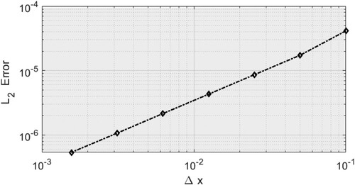
Table 1. $L_2$ error and CPU time consumed to arrive t = 25 for the numerical technique.

$\mathrm{\Delta }x$	$L_2$ error	CPU
1.0000e−01	4.1300e−05	$7.55\times {10}^{-3}$ s
5.0000e−02	1.7300e−05	$1.27\times {10}^{-2}$ s
2.5000e−02	8.6300e−06	$2.26\times {10}^{-2}$ s
1.2500e−02	4.3000e−06	$3.95\times {10}^{-2}$ s
6.2500e−03	2.1500e−06	$7.57\times {10}^{-2}$ s
3.1250e−03	1.0700e−06	$1.48\times {10}^{-1}$ s
1.5625e−03	5.3700e−07	$3.32\times {10}^{-1}$ s

7. Conclusion

To sum up, the Riccati–Bernoulli sub-ODE method has been successfully employed on the generalized Ito equation to establish its exact travelling wave and numerical solutions. Some exact travelling wave solutions have been expressed in forms of trigonometric and hyperbolic functions. The accomplished numerical solutions have been precisely compared with the obtained exact solutions, and we have recognized that both solutions almost coincide with each other. This can be easily observed in the presented figures. It can be pointed out that the suggested numerical technique provides reliable, successful and practical results. We have proved that the obtained exact solutions are stable on a specific interval with certain parameters. The Von Neumann stability has emphasized that the scheme is always stable. The accuracy of the schemes is the second order in time and space. The $L_2$ error dramatically diminishes for a tiny space size, as depicted in Figure 8. Ultimately, it can be deduced that the used techniques can be applied to more sophisticated nonlinear integro-differential equations.

Disclosure statement

No potential conflict of interest was reported by the author(s).

References

- Adomain G. Solving frontier problems of physics: the decomposition method. Boston (MA): Kluwer Academic Publishers; 1994.
- Wazwaz AM. Partial differential equations: method and applications. Lisse, Netherlands: Taylor and Francis; 2002.
- Wazwaz AM. Exact solutions to the double sinh-Gordon equation by the tanh method and a variable separated ODE method. Comput Math Appl. 2005;50:1685–1696.
- Wazwaz AM. A sine-cosine method for handling nonlinear wave equations. Math Comput Modelling. 2004;40:499–508.
- Feng X. Exploratory approach to explicit solution of nonlinear evolutions equations. Int J Theo Phys. 2000;39:207–222.
- Malflieta W, Hereman W. The tanh method: exact solutions of nonlinear evolution and wave equations. Phys Scr. 1996;54:563–568.
- Wazwaz AM. The tanh method for travelling wave solutions of nonlinear equations. Appl Math Comput. 2004;154:714–723.
- Fan E. Extended tanh-function method and its applications to nonlinear equations. Phys Lett A. 2000;277:212–218.
- Wazwaz AM. The extended tanh method for abundant solitary wave solutions of nonlinear wave equations. Appl Math Comput. 2007;187:1131–1142.
- Zayed EME, Abourabia AM, Gepreel KA, Horbaty MM. On the rational solitary wave solutions for the nonlinear HirotaCSatsuma coupled KdV system. Appl Anal. 2006;85:751–768.
- Chow KW. A class of exact periodic solutions of nonlinear envelope equation. J Math Phys. 1995;36:4125–4137.
- Zhao MM, Li C. The exp(−ϕ(ζ))-expansion method applied to nonlinear evolution equations. Available from: http://www.Paper.Edu.Cn.
- Alharbi AR, Almatrafi MB. Analytical and numerical solutions for the variant Boussinseq equations. J Taibah Univ Sci. 2020;14(1):454–462.
- Cesar A, Gomez S. New traveling waves solutions to generalized Kaup–Kupershmidt and Ito equations. Appl Math Comput. 2010;216:241–250.
- Alharbi AR, Almatrafi MB, Abdelrahman MAE. The extended Jacobian elliptic function expansion approach to the generalized fifth order kdV equation. J Phy Math. 2019;10(4):310.
- Alharbi AR, Almatrafi MB. Numerical investigation of the dispersive long wave equation using an adaptive moving mesh method and its stability. Results Phys. 2020;16:102870.
- Alharbi AR, Almatrafi MB. Riccati–Bernoulli sub-ODE approach on the partial differential equations and applications. Int J Math Comput Sci. 2020;15(1):367–388.
- Abdelrahman MAE, Almatrafi MB, Alharbi A. Fundamental solutions for the coupled KdV system and its stability. Symmetry. 2020;12:429.
- Alharbi A, Abdelrahman MAE, Almatrafi MB. Analytical and numerical investigation for the DMBBM equation. CMES. 2020;122(2):743–756.
- Alharbi A, Almatrafi MB, Abdelrahman MAE. Analytical and numerical investigation for Kadomtsev–Petviashvili equation arising in plasma physics. Phys Scr. 2020;95(4):045215.
- Alam MN, Tun** C. Constructions of the optical solitons and other solitons to the conformable fractional Zakharov–Kuznetsov equation with power law nonlinearity. J Taibah Univ Sci. 2019;14(1):94–100.
- Shahida N, Tun** C. Resolution of coincident factors in altering the flow dynamics of an MHD elastoviscous fluid past an unbounded upright channel. J Taibah Univ Sci. 2019;13(1):1022–1034.
- Seadawy AR, Iqbal M, Lu D. Nonlinear wave solutions of the Kudryashov–Sinelshchikov dynamical equation in mixtures liquid-gas bubbles under the consideration of heat transfer and viscosity. J Taibah Univ Sci. 2019;13(1):1060–1072.
- Ito M. An extension of nonlinear evolution equations of the KdV (mKdV) type to higher order. J. Phys. Soc. Jpn. 1980;49(2):771–778.
- Zhao Z, Dai Z, Han S, The EHTA for nonlinear evolution equations. Appl Math Comput. 2010;217:4306–4310.
- Seadawy A, Ali A, Aljahdaly N. The nonlinear integro-differential Ito dynamical equation via three modified mathematical methods and its analytical solutions. Open Phys. 2020;18:24–32.
- Akbari M. Application of Kudryashov method for the Ito equations. Appl. Appl. Math. 2017;12(1):136–142.
- Yang XF, Deng ZC, Wei Y. A Riccati–Bernoulli sub-ODE method for nonlinear partial differential equations and its application. Adv Differ Equ. 2015;1:117–133.
- Chandrasekhar S. Hydrodynamic and hydromagnetic stability. New York (NY): Dover Publications Inc; 1981.
- Sandstede B. Chapter 18 – stability of travelling waves. Handbook Dyn Syst. 2002;2:983–1055.
- Alharbi AR, Naire S. An adaptive moving mesh method for thin film flow equations with surface tension. J Comput Appl Math. 2017;319(4):365–384.
- Alharbi AR, Shailesh N. An adaptive moving mesh method for two-dimensional thin film flow equations with surface tension. J Comput Appl Math. 2019;356:219–230.
- Alharbi AR. Numerical solution of thin-film flow equations using adaptive moving mesh methods [PhD thesis]. Keele University; 2016.
- Brown PN, Hindmarsh AC, Petzold LE. Using Krylov methods in the solution of large-scale differential- algebraic systems. SIAM J Sci Comput. 1994;15:1467–1488.