Some newly explored exact solitary wave solutions to nonlinear inhomogeneous Murnaghan’s rod equation of fractional order

Abstract

The use of improved generalized Riccati equation mapping method has been demonstrated to find some new exact travelling wave solutions to space-time fractional non-liner double dispersive equation (DDE). The equation is used for modelling wave propagation in elastic inhomogeneous Murnaghan's rod. We have used Caputo's fractional derivative to achieve the fractional version of Murnaghan's rod equation. Improved generalized Riccati equation mapping method proves to be very effective tool to find a variety of soliton solutions. As a result, we found many new and general solutions including dark, combined dark-bright, singular periodic wave, combined singular periodic wave solutions and rational solutions. We have simulated the solitons, to check their types, with the help of graphs and all the solutions obtained in this article have been verified by back substitution in original equation by using Maple 17.

KEYWORDS:

• Improved generalized Riccati equation mapping method
• double dispersive equation
• inhomogeneous Murnaghan’s rod
• Caputo’s fractional derivative
• combined dark-bright solutions
• singular periodic wave solutions

1. Introduction

The use of fractional calculus to model certain real-life phenomena is getting a great attention nowadays. Nonlinear fractional differential equations (NLFDEs) appear as a direct result of this attention. Nonlinear fractional partial differential equations (NLFPDEs) cover a major share of those NLFDEs and they are used to model such phenomena where the dependent variable is reliant on more than one independent variable. NLFPDEs are generalization of nonlinear partial differential equations (NPDEs) in which the orders of derivatives involved are fractional. These equations have numerous applications in different fields of engineering and physical sciences such as in fluid mechanic, fractional dynamics, wave propagation and so on [1]. It is very important not only to formulate the governing nonlinear PDE of a certain phenomenon but also to find out its exact solutions. Solutions of an equation, governing a certain real-life phenomenon, give us very useful details of the phenomenon itself and can be used to understand and predict the variations in the depended variable (and the quantities driven by it). Many scientist and researchers have extensively studied nonlinear PDEs and their methods to construct exact solutions. Some of the important works are done in [2–13].

In this study, we are interested in a special type of exact solutions of NLFPDEs known as solitary wave solutions. Since solitons have been proved to be the exact solutions of a large class of NLPDEs, their complete understanding would lead us to a broad understanding of the real-life phenomena themselves. Some of the methods that are already being used to find solution of fractional order nonlinear partial differential equations are Homotopy perturbation method (HPM) [14], Lie algebra method [15,16], Variational iteration method (VIM) [17,18], F-expansion method [19], Exp-function method [20,21], Fan sub-equation method [22], $\left(\frac{G^{\mathrm{\prime }}}{G}\right)$-expansion method [23], Improved tan ($\frac{\varphi }{2}$)-expansion method [24], Exp $\left(-\varphi \left(\xi \right)\right)$ method [25], Kudryashov method [26], etc. Some of these methods provide exact solutions to NLFPDEs (like Exp-function method, Fan sub-equation method, $\left(\frac{G^{\mathrm{\prime }}}{G}\right)$-expansion method, etc.) while the others provide series solution (like VIM and HPM). Nowadays mathematicians are trying to extend conventional methods to make them capable of solving fractional order partial differential equations. These extended methods would enable scientist working on fractional models to deal with them more effectively. Finding exact solutions of NLFPDEs used to be a herculean task, however, with modern symbolic computation tools have make the task relatively easier. In a result of these computational tools, the efforts to extend the methods used to solve integer order NLPDEs to their fractional counterparts, and apply them to solve real-life fractional models, have gain a tremendous popularity.

Improved generalized Riccati equation method is one of the methods to the get exact traveling wave solutions to the PDEs having both steepening and spreading effects. It is a straight-forward and easy-to-use method that, by symbolic computation, can generate many different types of exact travelling wave solutions. Zhu [27] introduced this method with the extended tanh-function method to solve (2 + 1) dimensional Boiti–Leon–Pempinelle equation. Bekir and Cevikel [28] used Riccati equation combined with tanh–coth method to solve nonlinear coupled equation in mathematical physics. Li et al. [29] used this method to find exact solutions of (3 + 1)-dimensional Jimbo–Miwa equation. Tala-Tebue et al. [30] used this method to solve discrete nonlinear electrical transmission lines in (2 + 1) dimension. Salathiel et al. [31] utilized generalized Riccati equation mapping method to construct soliton and travelling wave solutions for discrete electrical lattice. Koonprasert et al. [32] implemented this method to find more explicit solitary solutions to the space–time fractional fifth-order nonlinear Sawada–Kotera equation. Most recently, Bibi et al. [33] have used this method on Caudrey–Dodd–Gibsson equation. Their work shows that the improved generalized Riccati equation method has a great protentional for solving fractional order partial differential equations. In this context, it seems appropriate to apply this method to some other real-life fractional models and obtain their unexplored exact travelling wave solutions.

The doubly dispersive equation (DDE) is an important nonlinear physical model describing the nonlinear wave propagation in the elastic inhomogeneous circular cylinder Murnaghan’s rod. It is an important model to study the wave propagation in nonlinear elastic solids. Solitary strain waves have great importance in the study of seismology, acoustics, introscopy, examination of sudden destruction, long distance energy transfer, vibro-impact treatments of hard materials also in studies for the development of non-destructive testing techniques especially for pipelines, and to understand the physical properties and internal structure of solids like brass, steel, glass and polymers. This relatively new area of study might increase interest in researchers to study nonlinear physics of solids, nonlinear mechanics and condensed matter physics [34]. The global existence and blow-up of solutions for doubly dispersive equation were discussed by Harby et al. [35]. Cattani et al. [36] had used extended Sinh-Gordon equation expansion method (ShGEEM) and the modified exp(−ϕ(ζ))-expansion function method, to find different types of solitary wave solutions. Moreover, Baskonus et al. [37] solved inhomogeneous Murnaghan’s rod by F-expansion method and obtained Jacobi elliptic function solutions including bright and dark solitons, topological, non-topological, singular, periodic, their combinations and compound solitons.

From the above references, it is clear that the solutions to DD equation (even of integer order) are a very recent topic and it still needs a lot exploration. Up to the best of our knowledge, no one has ever studied the fractional model for DD equation. To fill this gap, in this paper, we have used generalized Riccati equation method and able to construct abundant exact solutions (including solitary wave solutions, periodic wave solutions and rational solutions) to nonlinear DD equation (with space–time fractional derivatives) which describes wave propagation in nonlinear elastic inhomogeneous Murnaghan’s rod.

This paper is organized as follows: Section 1 includes introduction, Section 2 provides definition and properties of Caputo fractional derivative, in Section 3, improved generalized Riccati equation mapping method has been described briefly, Section 4 includes application of method described in Section 3 to obtain new solitary wave solutions of Murnaghan’s rod equation, Section 5 consists results and discussion on some of obtained results, Section 6 includes conclusion.

2. Definitions and properties of Caputo fractional derivative

Let $m$ be a smallest integer that is greater than $\alpha$, the Caputo time fractional derivative operator of order $\alpha >0$ of the function $u\left(t,\tau \right)$ is defined as follows [38]: (1) $\begin{array}{rl}{D}_t^{\alpha }f\left(t\right)& =\frac{{\mathrm{\partial }}^{\alpha }u\left(t,\tau \right)}{\mathrm{\partial }{t}^{\alpha }}\\ & =\left\{\begin{array}{l}\frac{1}{\mathrm{\Gamma }\left(m-\alpha \right)}\\ {\int }_0^t{(t-s)}^{m-\alpha -1}\frac{{\mathrm{\partial }}^{m}f\left(s\right)}{\mathrm{\partial }{s}^m}ds,& m-1<\alpha \le m,\\ \frac{{\mathrm{\partial }}^{m}u\left(t,\tau \right)}{\mathrm{\partial }{t}^m},& \alpha =m\in N,\end{array}\right.\end{array}$(1) Important characteristics of Caputo fractional derivative can be seen in [38] and keeping in view the length of the manuscript we see fit not to rewrite them here.

3. Improved generalized Riccati equation mapping method

Let us consider the fractional order differential equation with independent variables $x,t$ and some dependent function $u:$ (2) $\begin{array}{r}M\left(u,D_t^{\alpha }u,D_x^{\alpha }u,D_x^{2\alpha }u,D_x^{3\alpha }u,\dots \right)=0,0<\alpha \le 1,\end{array}$(2) where $D_t^{\alpha }$ and $D_x^{\alpha }$ are known as Caputo fractional derivatives of $u$ and $M$ is a polynomial in $u$ with its various orders of nonlinear partial fractional derivatives.

Step 1. Let (3) $\begin{array}{r}u\left(x,t\right)=U\left(\xi \right),\end{array}$(3) where (4) $\begin{array}{r}\xi =\frac{x^{\alpha }}{\mathrm{\Gamma }\left(1+\alpha \right)}-\frac{\lambda t^{\alpha }}{\mathrm{\Gamma }\left(1+\alpha \right)}\end{array}$(4) is a fractional complex transformation which can convert nonlinear fractional differential equation (2) into nonlinear ordinary differential equation, where $\lambda$ is a constant which is to be determined, this fractional complex transform is an easy transform to convert fractional differential equation into ordinary differential equation. As the classical chain rule does not hold for fractional derivatives, [39] introduced new chain rule in terms of $\sigma$ index and suggested that (5) $\begin{array}{rl}{D}_t^{\alpha }u& ={\sigma }_t^{\mathrm{\prime }}\frac{\text{d}U}{\text{d}\xi }{D}_t^{\alpha }\xi ,\\ D_x^{\alpha }u& ={\sigma }_x^{\mathrm{\prime }}\frac{\text{d}U}{\text{d}\xi }{D}_x^{\alpha }\xi ,\end{array}$(5) where ${\sigma }_t^{\mathrm{\prime }}$, ${\sigma }_x^{\mathrm{\prime }}$ are called sigma indexes [40], without loss of generality we can take ${\sigma }_t^{\mathrm{\prime }}={\sigma }_x^{\mathrm{\prime }}=c_0.$ Where $c_0$ is constant. By using the definition of Caputo derivative and applying the chain rule mentioned in Equation (5) along with complex transformation (4) into Equation (2) we get the following nonlinear ordinary differential equation. (6) $\begin{array}{r}{Q}^{\mathrm{\prime }}=Q^{\mathrm{\prime }}\left(U\left(\xi \right),U^{\mathrm{\prime }}\left(\xi \right),U^{\mathrm{\prime }\mathrm{\prime }}\left(\xi \right),\dots \right)=0,\end{array}$(6) where $U^{\mathrm{\prime }}\left(\xi \right)=\frac{\text{d}U\left(\xi \right)}{\text{d}\xi }$ indicates derivative in term of $\xi$. We integrate Equation (6) as many times as we get at least one term without derivative.

Step 2. We suppose that the following series expansion is the solution of Equation (6). (7) $\begin{array}{r}U\left(\xi \right)=\sum _{i=-N}^N{a}_i\varphi (\xi {)}^i,\end{array}$(7) where $a_i\left(i=0,\pm 1,\pm 2,\cdots \pm N\right)$ being constants, which are to be determined provided $a_i\ne 0.$ The function $\varphi =\varphi \left(\xi \right)$ satisfies the Riccati differential equation (8) $\begin{array}{rl}{\varphi }^{\mathrm{\prime }}\left(\xi \right)& =r+p\varphi \left(\xi \right)\\ & +q\varphi (\xi {)}^2,\text{where }r,p,q\text{ are real constants}\text{.}\end{array}$(8)

Step 3. Positive integer $N$ in Equation (7) can be found by using homogeneous balance between the derivatives of highest order and the nonlinear terms in Equation (6).

Step 4. Substituting Equation (7) along with Equation (8) into Equation (6) followed by collecting all the same order terms ${\varphi }^i$ together, we get the polynomial equation in ${\varphi }^i$ and ${\varphi }^{-i}$, where $\left(i=0,1,2,\dots \right).$ Equalizing coefficients of the resulting polynomial to zero, we get over-determined system of algebraic equations for $a_i$ where $i=0,\pm 1,\pm 2,\dots \pm N.$

Step 5. With the help of Maple, we solve the system described in step 4, and obtain $a_i$, where $i=0,\pm 1,\pm 2,\dots \pm N$. We substitute these values in Equation (7) coupled with solutions of Equation (8) and applying the transformation in Equation (6) we construct several exact solutions of Equation (2), establishing four families [32].

4. Implementation of proposed method to Murnaghan’s rod

In this section, we apply improved generalized Riccati equation mapping method on space–time fractional double dispersive equation which is given as (9) $\begin{array}{rl}& D_t^{2\alpha }u\left(x,t\right)-\frac{E}{\theta }{D}_x^{2\alpha }u\left(x,t\right)=\frac{ϵ}{2}(\frac{1}{\theta }\left(l\text{β}{D}_x^{2\alpha }{u}^2\right(x,t)\\ & +\theta {\nu }^2{D}_{tx}^{4\alpha }u\left(x,t\right)-b\delta {\nu }^2{D}_x^{4\alpha }u\left(x,t\right))),\end{array}$(9) where $u\left(x,t\right)$ is the strain wave function, $b=\frac{M}{E}<1,l=\frac{B}{E}$ are combinations of the constant scale factors, $ϵ$ is the small parameter, $\text{β}$ is the nonlinearity, $\theta$ is the density, $\delta =\frac{E}{\left(2\left(1+\nu \right)\right)},\nu$ is the Poisson coefficient, for details see [34–37]. Parameter $0<\alpha \le 1$ is the order of fractional time and space derivatives. Where $D_t^{\alpha }u$ and $D_x^{\alpha }u$ are the Caputo fractional derivative of $u$ with respect to $t$ and $x$ respectively. Now, consider the following nonlinear fractional order wave transformation: $\begin{array}{r}u\left(x,t\right)=U\left(\xi \right),\text{with}\xi =\frac{x^{\alpha }}{\mathrm{\Gamma }\left(1+\alpha \right)}-\frac{\lambda t^{\alpha }}{\mathrm{\Gamma }\left(1+\alpha \right)},\end{array}$ where $\lambda$ is constant. Substituting the above-mentioned transformation (incorporating Caputo’s fractional derivative of power function) and Equation (5) into Equation (9) we get the following nonlinear ODE: (10) $\begin{array}{rl}& \frac{ϵ{\upsilon }^2\left(-{\lambda }^2\theta +b\delta \right)}{\theta }\\ & \times (-\frac{l\text{β}{\left(U\left(\xi \right)\right)}^2}{2{\upsilon }^2\left(-{\lambda }^2\theta +b\delta \right)}+\frac{{\lambda }^2\theta U\left(\xi \right)}{ϵ{\upsilon }^2\left(-{\lambda }^2\theta +b\delta \right)}\\ & -\frac{EU\left(\xi \right)}{ϵ{\upsilon }^2\left(-{\lambda }^2\theta +b\delta \right)})\\ & +\frac{1}{2}\frac{ϵ{\upsilon }^2\left(-{\lambda }^2\theta +b\delta \right)U^{\mathrm{\prime }\mathrm{\prime }}\left(\xi \right)}{\theta }\\ & \times \left(-\frac{{\lambda }^2\theta }{-{\lambda }^2\theta +b\delta }+\frac{b\delta }{-{\lambda }^2\theta +b\delta }\right)=0,\end{array}$(10) by integrating Equation (10) and using homogeneous balance principle between the highest order derivative and nonlinearity yields $N=2.$ Therefore, Equation (10) has a solution (11) $\begin{array}{r}U\left(\xi \right)=\frac{a_{-2}}{{\left(\varphi \left(\xi \right)\right)}^2}+\frac{a_{-1}}{\varphi \left(\xi \right)}+a_0+a_1\varphi \left(\xi \right)+a_2(\varphi \left(\xi \right){)}^2,\end{array}$(11) now substituting Equation (11) along with Equation (8) into Equation (10) after collecting all terms with the same order in ${\varphi }^i$ and ${\varphi }^{-i}$, where $\left(i=0,1,2,\dots \right).$ and equating each coefficient to zero, we obtain a system of nonlinear algebraic equations. Solving these equations by using Maple 17, we get following non-trivial solutions:

Case 1: $\begin{array}{rl}{a}_1& =0,a_2=0,a_0=-2\frac{{\upsilon }^2\left(p^2+2rq\right)}{\text{β}l\left(2+ϵ\left(p^2-4rq\right){\upsilon }^2\right)},\end{array}$ $\begin{array}{rl}{a}_{-1}& =-\frac{\left(12E-12b\delta \right)pr{\upsilon }^2}{\text{β}l\left(2+ϵ\left(p^2-4rq\right){\upsilon }^2\right)},\\ a_{-2}& =-\frac{\left(12E-12b\delta \right)r^2{\upsilon }^2}{\text{β}l\left(2+ϵ\left(p^2-4rq\right){\upsilon }^2\right)},\end{array}$ (12) $\begin{array}{rl}\lambda & =\sqrt{\frac{b\delta ϵp^2{\upsilon }^2-4b\delta ϵqr{\upsilon }^2+2E}{\theta \left(ϵp^2{\upsilon }^2-4ϵqr{\upsilon }^2+2\right)}},\end{array}$(12) (13) $\begin{array}{rl}{U}_1\left(\xi \right)& =a_0+\frac{a_{-2}}{{\left(\varphi \left(\xi \right)\right)}^2}+\frac{a_{-1}}{\varphi \left(\xi \right)}\end{array}$(13)

Case 2: $\begin{array}{rl}{a}_1& =0,a_2=0,a_0=12\frac{qr{\upsilon }^2\left(E-b\delta \right)}{\text{β}\left(ϵ\left(p^2-4rq\right){\upsilon }^2-2\right)l},\\ a_{-1}& =\frac{\left(12E-12b\delta \right)pr{\upsilon }^2}{\text{β}\left(ϵ\left(p^2-4rq\right){\upsilon }^2-2\right)l},\\ a_{-2}& =12\frac{\left(E-b\delta \right)r^2{\upsilon }^2}{\text{β}\left(ϵ\left(p^2-4rq\right){\upsilon }^2-2\right)l},\end{array}$ (14) $\begin{array}{rl}\lambda & =\sqrt{-\frac{2E-b\delta ϵp^2{\upsilon }^2+4b\delta ϵqr{\upsilon }^2}{\theta \left(ϵp^2{\upsilon }^2-4ϵqr{\upsilon }^2-2\right)}},\end{array}$(14) (15) $\begin{array}{rl}{U}_2\left(\xi \right)& =a_0+\frac{a_{-2}}{{\left(\varphi \left(\xi \right)\right)}^2}+\frac{a_{-1}}{\varphi \left(\xi \right)}\end{array}$(15) Case 3: (16) $\begin{array}{rl}{a}_{-1}& =0,a_{-2}=0,a_0=-2\frac{{\upsilon }^2\left(p^2+2rq\right)\left(E-b\delta \right)}{\text{β}l\left(2+ϵ\left(p^2-4rq\right){\upsilon }^2\right)},\\ a_1& =-\frac{\left(12E-12b\delta \right)pq{\upsilon }^2}{\text{β}l\left(2+ϵ\left(p^2-4rq\right){\upsilon }^2\right)},\\ a_2& =-\frac{\left(12E-12b\delta \right)q^2{\upsilon }^2}{\text{β}l\left(2+ϵ\left(p^2-4rq\right){\upsilon }^2\right)},\\ \lambda & =\sqrt{\frac{b\delta ϵp^2{\upsilon }^2-4b\delta ϵqr{\upsilon }^2+2E}{\theta \left(ϵp^2{\upsilon }^2-4ϵqr{\upsilon }^2+2\right)}},\end{array}$(16) (17) $\begin{array}{rl}{U}_3\left(\xi \right)& =a_0+a_1\varphi \left(\xi \right)+a_2(\varphi \left(\xi \right){)}^2\end{array}$(17) Case 4: (18) $\begin{array}{rl}{a}_{-1}& =0,a_{-2}=0,a_0=12\frac{qr{\upsilon }^2\left(-b\delta +E\right)}{\text{β}\left(-2+ϵ\left(p^2-4rq\right){\upsilon }^2\right)l},\\ a_1& =\frac{\left(12E-12b\delta \right)pq{\upsilon }^2}{\text{β}\left(-2+ϵ\left(p^2-4rq\right){\upsilon }^2\right)l},\\ a_2& =\frac{\left(12E-12b\delta \right)q^2{\upsilon }^2}{\text{β}\left(-2+ϵ\left(p^2-4rq\right){\upsilon }^2\right)l},\\ \lambda & =\sqrt{-\frac{2E-b\delta ϵp^2{\upsilon }^2+4b\delta ϵqr{\upsilon }^2}{\theta \left(ϵp^2{\upsilon }^2-4ϵqr{\upsilon }^2-2\right)}},\end{array}$(18) (19) $\begin{array}{rl}{U}_4\left(\xi \right)& =a_0+a_1\varphi \left(\xi \right)+a_2(\varphi \left(\xi \right){)}^2\end{array}$(19)

According to the method the improved generalized Riccati equation mapping technique yield 27 solutions of the Riccati equation in Equation (8) incorporating four different families [32]. For the case 1, substituting the values from Equation (12) into Equation (13) along with the Riccati equations solutions, we can get following different types of solutions. Please note, in all the following solutions, these substitutions have been made to make the results more elegant: $\begin{array}{rl}D& =\sqrt{p^2-4qr},K=\sqrt{4qr-p^2},\end{array}$ $\begin{array}{rl}{\dot{B}}_1& =\frac{\left(-6b\delta +6E\right)p{\upsilon }^2}{l\left(2+ϵ\left(p^2-4qr\right){\upsilon }^2\right)\text{β}},\\ {\dot{B}}_2& =\frac{\left(-3b\delta +3E\right){\upsilon }^2}{l\left(2+ϵ\left(p^2-4qr\right){\upsilon }^2\right)\text{β}},\end{array}$ $\begin{array}{rl}{\dot{B^{\mathrm{\prime }}}}_1& =\frac{\left(-6b\delta +6E\right)p{\upsilon }^2}{l\left(-2+ϵ\left(p^2-4qr\right){\upsilon }^2\right)\text{β}},\\ {\dot{B^{\mathrm{\prime }}}}_2& =\frac{\left(-3b\delta +3E\right){\upsilon }^2}{l\left(-2+ϵ\left(p^2-4qr\right){\upsilon }^2\right)\text{β}}\end{array}$

Family 1:

When $p^2-4qr>0$ and $pq\ne 0$ or $qr\ne 0$, the hyperbolic function solutions of Equation (9) are as follows: (20) $\begin{array}{rl}{U}_{1,1}& =4{\dot{B}}_{1}rq{\left(\left(p+D\right)\tanh \left(\frac{1}{2D\xi }\right)\right)}^{-1}\\ & -16{\dot{B}}_2{r}^2{q}^2{\left(\left(p+D\right)\tanh \left(\frac{1}{2D\xi }\right)\right)}^{-2}+a_0,\end{array}$(20) (21) $\begin{array}{rl}{U}_{1,2}& =4{\dot{B}}_{1}rq{\left(\left(p+D\right)\coth \left(\frac{1}{2D\xi }\right)\right)}^{-1}\\ & -16{\dot{B}}_2{r}^2{q}^2{\left(\left(p+D\right)\coth \left(\frac{1}{2D\xi }\right)\right)}^{-2}+a_0,\end{array}$(21) (22) $\begin{array}{rl}{U}_{1,3}& =4{\dot{B}}_{1}rq(\left(p+D\right)\left(\text{tanh}\left(D\xi \right)\pm i\text{sech}\left(D\xi \right)\right){)}^{-1}\\ & -16{\dot{B}}_2{r}^2{q}^2\left(\right(p+D\left)\right(\tanh \left(D\xi \right)\\ & \pm i\text{sech}\left(D\xi \right)){)}^{-2}+a_0,\end{array}$(22) (23) $\begin{array}{rl}{U}_{1,4}& =4{\dot{B}}_{1}rq(\left(p+D\right)\left(\coth \left(D\xi \right)\pm \text{csch}\left(D\xi \right)\right){)}^{-1}\\ & -16{\dot{B}}_2{r}^2{q}^2\left(\right(p+D\left)\right(\coth \left(D\xi \right)\\ & \pm \text{csch}\left(D\xi \right)){)}^{-2}+a_0,\end{array}$(23) (24) $\begin{array}{rl}{U}_{1,5}& =4{\dot{B}}_{1}rq{\left(\left(2p+D\right)\left(2\text{coth}\left(\frac{D\xi }{2}\right)\right)\right)}^{-1}\\ & -16{\dot{B}}_2{r}^2{q}^2{\left(\left(2p+D\right)\left(2\text{coth}\left(\frac{D\xi }{2}\right)\right)\right)}^{-2}+a_0,\end{array}$(24) (25) $\begin{array}{rl}{U}_{1,6}& =-16{\dot{B}}_2{r}^2{q}^2\\ & \times {\left(-p+\frac{\begin{array}{c}\sqrt{(A^2+B^2)}D\\ -AD\cosh \left(D\xi \right)\end{array}}{A\text{sinh}\left(D\xi \right)+B}\right)}^{-2}\\ & -4{\dot{B}}_{1}rq{\left(-p+\frac{\begin{array}{c}\sqrt{(A^2+B^2)}D\\ -AD\cosh \left(D\xi \right)\end{array}}{A\text{sinh}\left(D\xi \right)+B}\right)}^{-1}+a_0,\end{array}$(25) (26) $\begin{array}{rl}{U}_{1,7}& =-16{\dot{B}}_2{r}^2{q}^2\\ & \times {\left(-p-\frac{\begin{array}{c}\sqrt{\left(-A^2+B^2\right)}D\\ +AD\sinh \left(D\xi \right)\end{array}}{A\text{cosh}\left(D\xi \right)+B}\right)}^{-2}\\ & -4{\dot{B}}_{1}rq{\left(-p-\frac{\begin{array}{c}\sqrt{\left(-A^2+B^2\right)}D\\ +AD\sinh \left(D\xi \right)\end{array}}{A\text{cosh}\left(D\xi \right)+B}\right)}^{-1}+a_0,\end{array}$(26) where two non-zero real constants A and B satisfies $A^2-B^2>0.$ (27) $\begin{array}{rl}{U}_{1,8}& =-\frac{{\dot{B}}_2{\left(D\sinh \left(\frac{D\xi }{2}\right)-p\text{cosh}\left(\frac{D\xi }{2}\right)\right)}^2}{\cosh {\left(\frac{D\xi }{2}\right)}^2}\\ & -\frac{{\dot{B}}_1\left(D\sinh \left(\frac{D\xi }{2}\right)-p\text{cosh}\left(\frac{D\xi }{2}\right)\right)}{\cosh \left(\frac{D\xi }{2}\right)}+a_0,\end{array}$(27) (28) $\begin{array}{rl}{U}_{1,9}& =\frac{{\dot{B}}_1\left(-D\cosh \left(\frac{D\xi }{2}\right)+p\text{sinh}\left(\frac{D\xi }{2}\right)\right)}{\sinh \left(\frac{D\xi }{2}\right)}\\ & -\frac{{\dot{B}}_2{\left(-D\cosh \left(\frac{D\xi }{2}\right)+p\text{sinh}\left(\frac{D\xi }{2}\right)\right)}^2}{{\left(\sinh \left(\frac{D\xi }{2}\right)\right)}^2}+a_0,\end{array}$(28) (29) $\begin{array}{rl}{U}_{1,10}& =-\frac{{\dot{B}}_2{\left(\left(D\text{sinh}\right(D\xi )-p(\cosh \left(D\xi \right)\pm iD)\right)}^2}{{\left(\cosh \left(\frac{D\xi }{2}\right)\right)}^2}\\ & -\frac{{\dot{B}}_1\left(\left(D\text{sinh}\right(D\xi )-p(\cosh \left(D\xi \right)\pm iD)\right)}{\cosh \left(\frac{D\xi }{2}\right)}+a_0,\end{array}$(29) (30) $\begin{array}{rl}{U}_{1,11}& =-\frac{{\dot{B}}_2{\left(\left(D\cosh \left(D\xi \right)\right)-p\text{sinh}\left(\left(D\xi \right)\pm D\right)\right)}^2}{{\left(\sinh \frac{D\xi }{2}\right)}^2}\\ & -\frac{{\dot{B}}_1\left(\left(D\cosh \left(D\xi \right)\right)-p\text{sinh}\left(D\xi \right)\pm D\left)\right)\right)}{\left(\sinh \frac{D\xi }{2}\right)}+a_0,\end{array}$(30) (31) $\begin{array}{rl}{U}_{1,12}& =-\frac{{\dot{B}}_2{\left(-p\sinh \left(\frac{D\xi }{2}\right)+2D\cosh {\left(\frac{D\xi }{4}\right)}^2-D\right)}^2}{\sinh {\left(\frac{D\xi }{2}\right)}^2}\\ & -\frac{\begin{array}{c}{\dot{B}}_1(-p\text{sinh}\left(\frac{D\xi }{2}\right)\\ +2D\cosh {\left(\frac{D\xi }{4}\right)}^2-D)\end{array}}{\sinh \left(\frac{D\xi }{2}\right)}+a_0\end{array}$(31)

Family 2:

If $p^2-4qr<0$ and $pq\ne 0\left(\text{or}qr\ne 0\right)$, we have the following trigonometric solutions: (32) $\begin{array}{rl}{U}_{1,13}& =-16{\dot{B}}_2{r}^2{q}^2{\left(-p+K\tan \left(\frac{K\xi }{2}\right)\right)}^{-2}\\ & -4{\dot{B}}_{1}rq{\left(-p+K\tan \left(\frac{K\xi }{2}\right)\right)}^{-1}+a_0,\end{array}$(32) (33) $\begin{array}{rl}{U}_{1,14}& =4{\dot{B}}_{1}rq{\left(p+K\cot \left(\frac{K\xi }{2}\right)\right)}^{-1}\\ & -16{\dot{B}}_2{r}^2{q}^2{\left(p+K\cot \left(\frac{K\xi }{2}\right)\right)}^{-2}+a_0,\end{array}$(33) (34) $\begin{array}{rl}{U}_{1,15}& =-16{\dot{B}}_2{r}^2{q}^2(\left(-p+K\right)\left(\tan \left(K\xi \right)\pm \sec \left(K\xi \right)\right){)}^{-2}\\ & -4{\dot{B}}_{1}rq(\left(-p+K\right)\left(\tan \left(K\xi \right)\pm \sec \left(K\xi \right)\right){)}^{-1}+a_0,\end{array}$(34) (35) $\begin{array}{rl}{U}_{1,16}& =4{\dot{B}}_{1}rq(\left(p+K\right)\cot \left(K\xi \right)\pm \csc \left(K\xi \right){)}^{-1}\\ & -16{\dot{B}}_2{r}^2{q}^2(\left(p+K\right)\cot \left(K\xi \right)\pm \csc \left(K\xi \right){)}^{-2}+a_0,\end{array}$(35) (36) $\begin{array}{rl}{U}_{1,17}& =-64{\dot{B}}_2{r}^2{q}^2{\left(\left(-2p+K\right)\left(-2\cot \left(\frac{K\xi }{2}\right)\right)\right)}^{-2}\\ & -8{\dot{B}}_{1}rq{\left(\left(-2p+K\right)\left(-2\cot \left(\frac{K\xi }{2}\right)\right)\right)}^{-1}+a_0,\end{array}$(36) (37) $\begin{array}{rl}{U}_{1,18}& =-16{\dot{B}}_2{r}^2{q}^2{\left(-p+\frac{\begin{array}{c}\sqrt{\left(A^2-B^2\right)}K\\ -AK\cos \left(K\xi \right)\end{array}}{A\text{sin}\left(K\xi \right)+B}\right)}^{-2}\\ & -4{\dot{B}}_{1}rq{\left(-p+\frac{\begin{array}{c}\sqrt{\left(A^2-B^2\right)}K\\ -AK\cos \left(K\xi \right)\end{array}}{A\text{sin}\left(K\xi \right)+B}\right)}^{-1}+a_0,\end{array}$(37) (38) $\begin{array}{rl}{U}_{1,19}& =-16{\dot{B}}_2{r}^2{q}^2{\left(-p+\frac{\begin{array}{c}\sqrt{\left(A^2-B^2\right)}K\\ +AD\cos \left(K\xi \right)\end{array}}{A\text{sin}\left(K\xi \right)+B}\right)}^{-2}\\ & -4{\dot{B}}_{1}rq{\left(-p+\frac{\begin{array}{c}\sqrt{\left(A^2-B^2\right)}K\\ +AD\cos \left(K\xi \right)\end{array}}{A\text{sin}\left(K\xi \right)+B}\right)}^{-1}+a_0,\end{array}$(38) where two non-zero real constants A and B satisfies $A^2-B^2>0.$ (39) $\begin{array}{rl}{U}_{1,20}& =\frac{{\dot{B}}_1\left(K\left(\sin \left(\frac{K\xi }{2}\right)+p\text{cos}\left(\frac{K\xi }{2}\right)\right)\right)}{\cos \left(\frac{K\xi }{2}\right)}\\ & -\frac{{\dot{B}}_2{\left(K\left(\sin \left(\frac{K\xi }{2}\right)+p\text{cos}\left(\frac{K\xi }{2}\right)\right)\right)}^2}{{\left(\cos \left(\frac{K\xi }{2}\right)\right)}^2}+a_0\end{array}$(39) (40) $\begin{array}{rl}{U}_{1,21}& =-\frac{{\dot{B}}_2{\left(K\left(\cos \left(\frac{K\xi }{2}\right)-p\text{sin}\left(\frac{K\xi }{2}\right)\right)\right)}^2}{{\left(\sin \left(\frac{K\xi }{2}\right)\right)}^2}\\ & -\frac{{\dot{B}}_1\left(K\left(\cos \left(\frac{K\xi }{2}\right)-p\text{sin}\left(\frac{K\xi }{2}\right)\right)\right)}{\sin \left(\frac{K\xi }{2}\right)}+a_0,\end{array}$(40) (41) $\begin{array}{rl}{U}_{1,22}& =\frac{{\dot{B}}_1\left(K\sin \left(K\xi \right)+p\cos \left(K\xi \right)\pm K\right)}{\cos \left(\frac{K\xi }{2}\right)}\\ & -\frac{{\dot{B}}_2{\left(K\sin \left(K\xi \right)+p\cos \left(K\xi \right)\pm K\right)}^2}{{\left(\cos \left(\frac{K\xi }{2}\right)\right)}^2}+a_0,\end{array}$(41) (42) $\begin{array}{rl}{U}_{1,23}& =-\frac{{\dot{B}}_2{\left(\left(K\cos \left(K\xi \right)\right)-p\text{sin}\left(K\xi \right)\pm K\right)}^2}{{\left(\sin \left(K\xi \right)\right)}^2}\\ & -\frac{{\dot{B}}_1\left(\left(K\cos \left(K\xi \right)\right)-p\text{sin}\left(K\xi \right)\pm K\right)}{\sin \left(K\xi \right)}+a_0,\end{array}$(42) (43) $\begin{array}{rl}{U}_{1,24}& =-\frac{{\dot{B}}_2{\left(\left(-p\sin \left(\frac{K\xi }{2}\right)\right)+2K{\left(\cos \left(\frac{K\xi }{4}\right)\right)}^2-K\right)}^2}{{\left(\sin \left(\frac{K\xi }{2}\right)\right)}^2}\\ & -\frac{\begin{array}{c}{\dot{B}}_1(\left(-p\sin \left(\frac{K\xi }{2}\right)\right)\\ +2K{\left(\cos \left(\frac{K\xi }{4}\right)\right)}^2-K)\end{array}}{\sin \left(\frac{K\xi }{2}\right)}+a_0,\end{array}$(43)

For case 2, we have following solutions.

Family 1:

The hyperbolic function solutions of Equation (9) (when $p^2-4qr>0$ and $pq\ne 0$ or $qr\ne 0$) are: (44) $\begin{array}{rl}{U}_{2,1}& =16{\dot{B^{\mathrm{\prime }}}}_2{r}^2{q}^2{\left(p+\left(D\tanh \left(\frac{D\xi }{2}\right)\right)\right)}^{-2}\\ & -4{\dot{B^{\mathrm{\prime }}}}_{1}rq{\left(p+\left(D\tanh \left(\frac{D\xi }{2}\right)\right)\right)}^{-1}+a_0,\end{array}$(44) (45) $\begin{array}{rl}{U}_{2,2}& =16{\dot{B^{\mathrm{\prime }}}}_2{r}^2{q}^2{\left(p+\left(D\coth \left(\frac{D\xi }{2}\right)\right)\right)}^{-2}\\ & -4{\dot{B^{\mathrm{\prime }}}}_{1}rq{\left(p+\left(D\coth \left(\frac{D\xi }{2}\right)\right)\right)}^{-1}+a_0,\end{array}$(45) (46) $\begin{array}{rl}{U}_{2,3}& =16{\dot{B^{\mathrm{\prime }}}}_2{r}^2{q}^2(\left(p+D\right)\left(\tanh \left(D\xi \right)\pm i\text{sech}\left(D\xi \right)\right){)}^{-2}\\ & -4{\dot{B^{\mathrm{\prime }}}}_{1}rq\left(\right(p+D\left)\right(\tanh \left(D\xi \right)\\ & \pm i\text{sech}\left(D\xi \right)){)}^{-1}+a_0,\end{array}$(46) (47) $\begin{array}{rl}{U}_{2,4}& =16{{\dot{B}}^{\mathrm{\prime }}}_2{r}^2{q}^2(\left(p+D\right)\left(\coth \left(D\xi \right)\pm \text{csch}\left(D\xi \right)\right){)}^{-2}\\ & -4{\dot{B^{\mathrm{\prime }}}}_{1}rq\left(\right(p+D\left)\right(\coth \left(D\xi \right)\\ & \pm \text{csch}\left(D\xi \right)){)}^{-1}+a_0,\end{array}$(47) (48) $\begin{array}{rl}{U}_{2,5}& =16{{\dot{B}}^{\mathrm{\prime }}}_2{r}^2{q}^2{\left(\left(2p+D\right)\left(2\coth \left(\frac{D\xi }{2}\right)\right)\right)}^{-2}\\ & -4{\dot{B^{\mathrm{\prime }}}}_{1}rq{\left(\left(2p+D\right)\left(2\coth \left(\frac{D\xi }{2}\right)\right)\right)}^{-1}+a_0,\end{array}$(48) (49) $\begin{array}{rl}{U}_{2,6}& =16{{\dot{B}}^{\mathrm{\prime }}}_2{r}^2{q}^2{\left(-p+\frac{\begin{array}{c}\sqrt{\left(A^2+B^2\right)}D\\ -AD\cosh \left(D\xi \right)\end{array}}{A\text{sinh}\left(D\xi \right)+B}\right)}^{-2}\\ & +4{{\dot{B}}^{\mathrm{\prime }}}_{1}rq{\left(-p+\frac{\begin{array}{c}\sqrt{\left(A^2+B^2\right)}D\\ -AD\cosh \left(D\xi \right)\end{array}}{A\text{sinh}\left(D\xi \right)+B}\right)}^{-1}+a_0,\end{array}$(49) (50) $\begin{array}{rl}{U}_{2,7}& =16{\dot{B}}_2{r}^2{q}^2{\left(-p-\frac{\begin{array}{c}\sqrt{\left(-A^2+B^2\right)}D\\ +AD\cosh \left(D\xi \right)\end{array}}{A\text{cosh}\left(D\xi \right)+B}\right)}^{-2}\\ & +4{{\dot{B}}^{\mathrm{\prime }}}_{1}rq{\left(-p-\frac{\begin{array}{c}\sqrt{\left(-A^2+B^2\right)}D\\ +AD\cosh \left(D\xi \right)\end{array}}{A\text{cosh}\left(D\xi \right)+B}\right)}^{-1}+a_0,\end{array}$(50)

Where two non-zero real constants $A$ and $B$ satisfy $A^2-B^2>0.$ (51) $\begin{array}{rl}{U}_{2,8}& =\frac{{{\dot{B}}^{\mathrm{\prime }}}_2{\left(D\sinh \left(\frac{D\xi }{2}\right)-p\text{cosh}\left(\frac{D\xi }{2}\right)\right)}^2}{{\left(\cosh \left(\frac{D\xi }{2}\right)\right)}^2}\\ & +\frac{{{\dot{B}}^{\mathrm{\prime }}}_1\left(D\sinh \left(\frac{D\xi }{2}\right)-p\text{cosh}\left(\frac{D\xi }{2}\right)\right)}{\cosh \left(\frac{D\xi }{2}\right)}+a_0,\end{array}$(51) (52) $\begin{array}{rl}{U}_{2,9}& =\frac{{{\dot{B}}^{\mathrm{\prime }}}_2{\left(-D\cosh \left(\frac{D\xi }{2}\right)+p\text{sinh}\left(\frac{D\xi }{2}\right)\right)}^2}{{\left(\sinh \left(\frac{D\xi }{2}\right)\right)}^2}\\ & -\frac{{\dot{B^{\mathrm{\prime }}}}_1\left(-D\cosh \left(\frac{D\xi }{2}\right)+p\text{sinh}\left(\frac{D\xi }{2}\right)\right)}{\sinh \left(\frac{D\xi }{2}\right)}+a_0,\end{array}$(52) (53) $\begin{array}{rl}{U}_{2,10}& =\frac{{\dot{B^{\mathrm{\prime }}}}_2{\left(D\sinh \left(D\xi \right)-p\left(\cosh \left(D\xi \right)\pm iD\right)\right)}^2}{{\left(\cosh \left(\frac{1}{2D\xi }\right)\right)}^2}\\ & +\frac{{\dot{B^{\mathrm{\prime }}}}_1\left(D\sinh \left(D\xi \right)-p\left(\cosh \left(D\xi \right)\pm iD\right)\right)}{\cosh \left(\frac{1}{2D\xi }\right)}+a_0,\end{array}$(53) (54) $\begin{array}{rl}{U}_{2,11}& =\frac{{{\dot{B}}^{\mathrm{\prime }}}_2{\left(D\cosh \left(D\xi \right)-p\left(\sinh \left(D\xi \right)\pm D\right)\right)}^2}{{\left(\sinh \left(\frac{D\xi }{2}\right)\right)}^2}\\ & +\frac{{\dot{B^{\mathrm{\prime }}}}_1\left(D\cosh \left(D\xi \right)-p\left(\sinh \left(D\xi \right)\pm D\right)\right)}{\sinh \left(\frac{D\xi }{2}\right)}+a_0,\end{array}$(54) (55) $\begin{array}{rl}{U}_{2,12}& =\frac{\begin{array}{c}{{\dot{B}}^{\mathrm{\prime }}}_2(\left(-p\sinh \left(\frac{D\xi }{2}\right)\right)+2D{\left(\cosh \left(\frac{1}{4D\xi }\right)\right)}^2\\ -D+2D{\left(\cosh \left(\frac{1}{4D\xi }\right)\right)}^2-D{)}^2\end{array}}{{\left(\sinh \left(\frac{D\xi }{2}\right)\right)}^2}\\ & +\frac{\begin{array}{c}{{\dot{B}}^{\mathrm{\prime }}}_1(\left(-p\sinh \left(\frac{D\xi }{2}\right)\right)\\ +2D{\left(\cosh \left(\frac{1}{4D\xi }\right)\right)}^2\\ -D+2D{\left(\cosh \left(\frac{1}{4D\xi }\right)\right)}^2-D)\end{array}}{\sinh \left(\frac{D\xi }{2}\right)}+a_0\end{array}$(55)

Family 2:

The trigonometric solutions of Equation (9) (if $p^2-4qr<0$ and $pq\ne 0\left(\text{or}qr\ne 0\right)$) are: (56) $\begin{array}{rl}{U}_{2,13}& =16{\dot{B}}_2^{\mathrm{\prime }}{r}^2{q}^2{\left(-p+K\tan \left(\frac{K\xi }{2}\right)\right)}^{-2}\\ & +4{\dot{B^{\mathrm{\prime }}}}_{1}rq{\left(-p+K\tan \left(\frac{K\xi }{2}\right)\right)}^{-1}+a_0,\end{array}$(56) (57) $\begin{array}{rl}{U}_{2,14}& =16{\dot{B^{\mathrm{\prime }}}}_2{r}^2{q}^2{\left(p+K\cot \left(\frac{K\xi }{2}\right)\right)}^{-2}\\ & -4{\dot{B^{\mathrm{\prime }}}}_{1}rq{\left(p+K\cot \left(\frac{K\xi }{2}\right)\right)}^{-1}+a_0,\end{array}$(57) (58) $\begin{array}{rl}{U}_{2,15}& =16{\dot{B}}_2^{\mathrm{\prime }}{r}^2{q}^2{\left(\begin{array}{c}\left(-p+K\right)\times \\ \left(\tan \left(K\xi \right)\pm \sec \left(K\xi \right)\right)\end{array}\right)}^{-2}\\ & +4{\dot{B^{\mathrm{\prime }}}}_{1}rq{\left(\begin{array}{c}\left(-p+K\right)\times \\ \left(\tan \left(K\xi \right)\pm \sec \left(K\xi \right)\right)\end{array}\right)}^{-1}-a_0,\end{array}$(58) (58a) $\begin{array}{rl}{U}_{2,16}& =16{\dot{B}}_2^{\mathrm{\prime }}{r}^2{q}^2{\left(\begin{array}{c}(p+K)\times \\ \left(\cot \left(K\xi \right)\pm \csc \left(K\xi \right)\right)\end{array}\right)}^{-2}\\ & -4{\dot{B^{\mathrm{\prime }}}}_{1}rq{\left(\begin{array}{c}\left(p+K\right)\times \\ \left(\cot \left(K\xi \right)\pm \csc \left(K\xi \right)\right)\end{array}\right)}^{-1}+a_0,\end{array}$(58a) (59) $\begin{array}{rl}{U}_{2,17}& =64{\dot{B^{\mathrm{\prime }}}}_2{r}^2{q}^2{\left(\left(-2p+K\right)\left(-2\cot \left(\frac{K\xi }{2}\right)\right)\right)}^{-2}\\ & +8{{\dot{B}}^{\mathrm{\prime }}}_{1}rq{\left(\left(-2p+K\right)\left(-2\cot \left(\frac{K\xi }{2}\right)\right)\right)}^{-1}+a_0,\end{array}$(59) (60) $\begin{array}{rl}{U}_{2,18}& =16{\dot{B^{\mathrm{\prime }}}}_2{r}^2{q}^2\\ & \times {\left(-p+\frac{\pm i\sqrt{\left(-A^2+B^2\right)}K-AK\cos \left(K\xi \right)}{A\text{sin}\left(K\xi \right)+B}\right)}^{-2}\\ & +4{\dot{B^{\mathrm{\prime }}}}_{1}rq\\ & \times {\left(-p+\frac{\pm i\sqrt{\left(-A^2+B^2\right)}K-AK\cos \left(K\xi \right)}{A\text{sin}\left(K\xi \right)+B}\right)}^{-1}+a_0,\end{array}$(60) (61) $\begin{array}{rl}{U}_{2,19}& =16{{\dot{B}}^{\mathrm{\prime }}}_2{r}^2{q}^2\\ & {\left(-p+\frac{\pm i\sqrt{\left(-A^2+B^2\right)}K+AK\cos \left(K\xi \right)}{A\text{sin}\left(K\xi \right)+B}\right)}^{-2}\\ & +4{\dot{B^{\mathrm{\prime }}}}_{1}rq\\ & {\left(-p+\frac{\pm i\sqrt{\left(-A^2+B^2\right)}K+AK\cos \left(K\xi \right)}{A\text{sin}\left(K\xi \right)+B}\right)}^{-1}+a_0,\end{array}$(61) where two non-zero real constants $A$ and $B$ satisfies $A^2-B^2>0.$ (62) $\begin{array}{rl}{U}_{2,20}& =\frac{{\dot{B^{\mathrm{\prime }}}}_2{\left(K\sin \left(\frac{K\xi }{2}\right)+p\text{cos}\left(\frac{K\xi }{2}\right)\right)}^2}{{\left(\cos \left(\frac{K\xi }{2}\right)\right)}^2}\\ & -\frac{{\dot{B^{\mathrm{\prime }}}}_1\left(K\sin \left(\frac{K\xi }{2}\right)+p\text{cos}\left(\frac{K\xi }{2}\right)\right)}{\cos \left(\frac{K\xi }{2}\right)}+a_0,\end{array}$(62) (63) $\begin{array}{rl}{U}_{2,21}& =\frac{{{\dot{B}}^{\mathrm{\prime }}}_2{\left(K\cos \left(\frac{K\xi }{2}\right)-p\text{sin}\left(\frac{K\xi }{2}\right)\right)}^2}{{\left(\sin \left(\frac{K\xi }{2}\right)\right)}^2}\\ & +\frac{{\dot{B^{\mathrm{\prime }}}}_1\left(K\cos \left(\frac{K\xi }{2}\right)-p\text{sin}\left(\frac{K\xi }{2}\right)\right)}{\sin \left(\frac{K\xi }{2}\right)}+a_0,\end{array}$(63) (64) $\begin{array}{rl}{U}_{2,22}& =\frac{{{\dot{B}}^{\mathrm{\prime }}}_2{\left(K\sin \left(K\xi \right)+p\cos \left(K\xi \right)\pm K\right)}^2}{{\left(\cos \left(\frac{K\xi }{2}\right)\right)}^2}\\ & -\frac{{\dot{B^{\mathrm{\prime }}}}_1\left(K\sin \left(K\xi \right)+p\cos \left(K\xi \right)\pm K\right)}{\cos \left(\frac{K\xi }{2}\right)}+a_0,\end{array}$(64) (65) $\begin{array}{rl}{U}_{2,23}& =\frac{{\dot{B^{\mathrm{\prime }}}}_2{\left(K\cos \left(K\xi \right)-p\sin \left(K\xi \right)\pm K\right)}^2}{{\left(\sin \left(K\xi \right)\right)}^2}\\ & +\frac{{{\dot{B}}^{\mathrm{\prime }}}_1\left(K\cos \left(K\xi \right)-p\sin \left(K\xi \right)\pm K\right)}{\sin \left(K\xi \right)}+a_0,\end{array}$(65) (66) $\begin{array}{rl}{U}_{2,24}& =a_0+{\dot{B^{\mathrm{\prime }}}}_2\frac{{\left(-p\sin \left(\frac{K\xi }{2}\right)+2K{\left(\cos \left(\frac{K\xi }{4}\right)\right)}^2-K)\right)}^2}{{\left(\sin \left(\frac{K\xi }{2}\right)\right)}^2}\\ & +{\dot{B^{\mathrm{\prime }}}}_1\frac{\left(-p\sin \left(\frac{K\xi }{2}\right)+2K{\left(\cos \left(\frac{K\xi }{4}\right)\right)}^2-K)\right)}{\sin \left(\frac{K\xi }{2}\right)},\end{array}$(66)

For case 3, we have

Family 1:

When $p^2-4qr>0$ and $pq\ne 0$ or $qr\ne 0$, we have (67) $\begin{array}{rl}{U}_{3,1}& ={\dot{B}}_1\left(p+D\tanh \left(\frac{D\xi }{2}\right)\right)\\ & -{\dot{B}}_2{\left(p+D\tanh \left(\frac{D\xi }{2}\right)\right)}^2+a_0,\end{array}$(67) (68) $\begin{array}{rl}{U}_{3,2}& ={\dot{B}}_1\left(p+D\coth \left(\frac{D\xi }{2}\right)\right)\\ & -{\dot{B}}_2{\left(p+D\coth \left(\frac{D\xi }{2}\right)\right)}^2+a_0,\end{array}$(68) (69) $\begin{array}{rl}{U}_{3,3}& ={\dot{B}}_1\left(\begin{array}{c}\left(p+D\right)\times \\ \left(\tanh \left(D\xi \right)\pm i\text{sech}\left(D\xi \right)\right)\end{array}\right)\\ & -{\dot{B}}_2{\left(\begin{array}{c}\left(p+D\right)\times \\ \tanh \left(D\xi \pm i\text{sech}\left(D\xi \right)\right)\end{array}\right)}^2+a_0,\end{array}$(69) (70) $\begin{array}{rl}{U}_{3,4}& ={\dot{B}}_1\left(\begin{array}{c}\left(p+D\right)\times \\ \left(\coth \left(D\xi \right)\pm \text{csch}\left(D\xi \right)\right)\end{array}\right)\\ & -{\dot{B}}_2{\left(\begin{array}{c}\left(p+D\right)\times \\ \left(\coth \left(D\xi \right)\pm \text{csch}\left(D\xi \right)\right)\end{array}\right)}^2+a_0,\end{array}$(70) (71) $\begin{array}{rl}{U}_{3,5}& ={\dot{B}}_1\left(2\left(2p+D\right)\coth \left(\frac{D\xi }{2}\right)\right)\\ & -{\dot{B}}_2{\left(2\left(2p+D\right)\coth \left(\frac{D\xi }{2}\right)\right)}^2+a_0,\end{array}$(71) (72) $\begin{array}{rl}{U}_{3,6}& =-{\dot{B}}_1\left(-p+\frac{\sqrt{\left(A^2+B^2\right)}D-AD\cosh \left(D\right)}{A\text{sinh}\left(D\right)+B}\right)\\ & -{\dot{B}}_2{\left(-p+\frac{\sqrt{\left(A^2+B^2\right)}D-AD\cosh \left(D\right)}{A\text{sinh}\left(D\right)+B}\right)}^2+a_0,\end{array}$(72) (73) $\begin{array}{rl}{U}_{3,7}& =-{\dot{B}}_1\left(-p-\frac{\sqrt{\left(-A^2+B^2\right)}D+AD\sinh \left(D\xi \right)}{A\text{cosh}\left(D\xi \right)+B}\right)\\ & -{\dot{B}}_2{\left(-p-\frac{\sqrt{\left(-A^2+B^2\right)}D+AD\sinh \left(D\xi \right)}{A\text{cosh}\left(D\xi \right)+B}\right)}^2+a_0,\end{array}$(73) where two non-zero real constants A and B satisfies $A^2-B^2>0.$ (74) $\begin{array}{rl}{U}_{3,8}& =-\frac{4{\dot{B}}_{1}qr\text{cosh}\left(\frac{D\xi }{2}\right)}{\left(D\sinh \left(\frac{D\xi }{2}\right)-p\text{cosh}\left(\frac{D\xi }{2}\right)\right)}\\ & -\frac{16{\dot{B}}_2{q}^2{r}^2{\left(\cosh \left(\frac{D\xi }{2}\right)\right)}^2}{{\left(D\sinh \left(\frac{D\xi }{2}\right)-p\text{cosh}\left(\frac{D\xi }{2}\right)\right)}^2}+a_0,\end{array}$(74) (75) $\begin{array}{rl}{U}_{3,9}& =\frac{4{\dot{B}}_{1}qr\text{sinh}\left(\frac{D\xi }{2}\right)}{\left(-D\cosh \left(\frac{D\xi }{2}\right)+p\text{sinh}\left(\frac{D\xi }{2}\right)\right)}\\ & -\frac{16{\dot{B}}_2{q}^2{r}^2{\left(\sinh \left(\frac{D\xi }{2}\right)\right)}^2}{{\left(-D\cosh \left(\frac{D\xi }{2}\right)+p\text{sinh}\left(\frac{D\xi }{2}\right)\right)}^2}+a_0,\end{array}$(75) (76) $\begin{array}{rl}{U}_{3,10}& =\frac{-4{\dot{B}}_{1}qr\text{cosh}\left(\frac{D\xi }{2}\right)}{\left(D\sinh \left(\omega \right)-p\left(\text{cosh}\right(D\xi )\pm iD\right)}\\ & -\frac{{\dot{B}}_2{q}^2{r}^2{\left(\cosh \left(\frac{D\xi }{2}\right)\right)}^2}{{\left(D\sinh \left(\omega \right)-p\left(\text{cosh}\right(D\xi )\pm iD\right)}^2}+a_0,\end{array}$(76) (77) $\begin{array}{rl}{U}_{3,11}& =\frac{-4{\dot{B}}_{1}qr\text{sinh}\left(\frac{D\xi }{2}\right)}{\left(D\cosh \left(D\xi \right)-p\left(\sinh \left(D\xi \right)\pm D\right)\right)}\\ & -\frac{16{\dot{B}}_2{q}^2{r}^2{\left(\sinh \left(\frac{D\xi }{2}\right)\right)}^2}{{\left(D\cosh \left(D\xi \right)-p\left(\sinh \left(D\xi \right)\pm D\right)\right)}^2}+a_0,\end{array}$(77) (78) $\begin{array}{rl}{U}_{3,12}& =-\frac{4{\dot{B}}_{1}qr\text{sinh}\left(\frac{D\xi }{2}\right)}{\left(-p\sinh \left(\frac{D\xi }{2}\right)+2D{\left(\cosh \left(\frac{D\xi }{4}\right)\right)}^2-D\right)}\\ & -\frac{16{\dot{B}}_2{q}^2{r}^2{\left(\sinh \left(\frac{D\xi }{2}\right)\right)}^2}{\begin{array}{c}(\left(-p\sinh \left(\frac{D\xi }{2}\right)\right)\\ +2D{\left(\cosh \left(\frac{D\xi }{4}\right)\right)}^2-D{)}^2\end{array}}+a_0,\end{array}$(78)

Family 2:

If $p^2-4qr<0$ and $pq\ne 0\left(\text{or}qr\ne 0\right)$, we have the following solutions: (79) $\begin{array}{rl}{U}_{3,13}& =-{\dot{B}}_1\left(-p+K\tan \left(\frac{K\xi }{2}\right)\right)\\ & -{\dot{B}}_2{\left(-p+K\tan \left(\frac{K\xi }{2}\right)\right)}^2+a_0,\end{array}$(79) (80) $\begin{array}{rl}{U}_{3,14}& ={\dot{B}}_1\left(p+K\cot \left(\frac{K\xi }{2}\right)\right)\\ & -{\dot{B}}_2{\left(p+K\cot \left(\frac{K\xi }{2}\right)\right)}^2+a_0,\end{array}$(80) (81) $\begin{array}{rl}{U}_{3,15}& =-{\dot{B}}_1\left(\begin{array}{c}\left(-p+K\right)\times \\ \left(\tan \left(K\xi \right)\pm \sec \left(K\xi \right)\right)\end{array}\right)\\ & -{\dot{B}}_2{\left(\begin{array}{c}\left(-p+K\right)\times \\ \left(\tan \left(K\xi \right)\pm \sec \left(K\xi \right)\right)\end{array}\right)}^2+a_0,\end{array}$(81) (82) $\begin{array}{rl}{U}_{3,16}& ={\dot{B}}_1\left(\begin{array}{c}\left(p+K\right)\times \\ \left(\cot \left(K\xi \right)\pm \csc \left(K\xi \right)\right)\end{array}\right)\\ & -{\dot{B}}_2{\left(\begin{array}{c}\left(p+K\right)\times \\ \left(\cot \left(K\xi \right)\pm \csc \left(K\xi \right)\right)\end{array}\right)}^2+a_0,\end{array}$(82) (83) $\begin{array}{rl}{U}_{3,17}& =-{\dot{B}}_1\left(\left(-2p+K\right)\left(-2\cot \left(\frac{K\xi }{2}\right)\right)\right)\\ & -{\dot{B}}_2{\left(\left(-2p+K\right)\left(-2\cot \left(\frac{K\xi }{2}\right)\right)\right)}^2+a_0,\end{array}$(83) (84) $\begin{array}{rl}{U}_{3,18}& =-{\dot{B}}_1\left(-p+\frac{\pm i\sqrt{\left(-A^2+B^2\right)}K-AK\cos \left(K\xi \right)}{A\text{sin}\left(K\xi \right)+B}\right)\\ & -{\dot{B}}_2{\left(-p+\frac{\pm i\sqrt{\left(-A^2+B^2\right)}K-AK\cos \left(K\xi \right)}{A\text{sin}\left(K\xi \right)+B}\right)}^2+a_0,\end{array}$(84) (85) $\begin{array}{rl}{U}_{3,19}& =-{\dot{B}}_1\left(-p+\frac{\pm i\sqrt{\left(-A^2+B^2\right)}K+AK\cos \left(K\xi \right)}{A\text{sin}\left(K\xi \right)+B}\right)\\ & -{\dot{B}}_2{\left(-p+\frac{\pm i\sqrt{\left(-A^2+B^2\right)}K+AK\cos \left(K\xi \right)}{A\text{sin}\left(K\xi \right)+B}\right)}^2+a_0,\end{array}$(85) where two non-zero real constants A and B satisfies $A^2-B^2>0.$ (86) $\begin{array}{rl}{U}_{3,20}& =\frac{4{\dot{B}}_{1}qr\text{cos}\left(\frac{K\xi }{2}\right)}{\left(K\sin \left(\frac{K\xi }{2}\right)+p\text{cos}\left(\frac{K\xi }{2}\right)\right)}\\ & -\frac{16{\dot{B}}_2{q}^2{r}^2{\left(\cos \left(\frac{K\xi }{2}\right)\right)}^2}{{\left(K\sin \left(\frac{K\xi }{2}\right)+p\text{cos}\left(\frac{K\xi }{2}\right)\right)}^2}+a_0,\end{array}$(86) (87) $\begin{array}{rl}{U}_{3,21}& =-\frac{4{\dot{B}}_{1}qr\text{sin}\left(\frac{K\xi }{2}\right)}{\left(K\cos \left(\frac{K\xi }{2}\right)-p\text{sin}\left(\frac{K\xi }{2}\right)\right)}\\ & -\frac{16{\dot{B}}_2{q}^2{r}^2{\left(\sin \left(\frac{K\xi }{2}\right)\right)}^2}{{\left(K\cos \left(\frac{K\xi }{2}\right)-p\text{sin}\left(\frac{K\xi }{2}\right)\right)}^2}+a_0,\end{array}$(87) (88) $\begin{array}{rl}{U}_{3,22}& =\frac{4{\dot{B}}_{1}qr\text{cos}\left(\frac{K\xi }{2}\right)}{\left(K\sin \left(K\xi \right)+p\cos \left(K\xi \right)\pm K\right)}\\ & -\frac{16{\dot{B}}_2{q}^2{r}^2{\left(\cos \left(\frac{K\xi }{2}\right)\right)}^2}{{\left(K\sin \left(K\xi \right)+p\cos \left(K\xi \right)\pm \xi \right)}^2}+a_0,\end{array}$(88) (89) $\begin{array}{rl}{U}_{3,23}& =-\frac{4{\dot{B}}_{1}q{\upsilon }^{2}r\text{sin}\left(K\xi \right)}{\left(\begin{array}{c}\sqrt{4qr-p^2}\cos \left(K\xi \right)-p\sin \left(K\xi \right)\pm K\end{array}\right)}\\ & -\frac{16{\dot{B}}_2{q}^2{r}^2{\left(\sin \left(K\xi \right)\right)}^2}{{\left(\begin{array}{c}K\cos \left(K\xi \right)\\ -p\sin \left(K\xi \right)\pm K\end{array}\right)}^2}+a_0,\end{array}$(89) (90) $\begin{array}{rl}{U}_{3,24}& =-\frac{4{\dot{B}}_{1}q{\upsilon }^{2}r\text{sin}\left(\frac{K\xi }{2}\right)}{\left(-p\sin \left(\frac{K\xi }{2}\right)+2K{\left(\cos \left(\frac{K\xi }{4}\right)\right)}^2-K\right)}\\ & -\frac{4{\dot{B}}_2{q}^2{r}^2{\left(\sin \left(\frac{K\xi }{2}\right)\right)}^2}{{\left(-p\sin \left(\frac{K\xi }{2}\right)+2K{\left(\cos \left(\frac{K\xi }{4}\right)\right)}^2-K\right)}^2}+a_0,\end{array}$(90)

Family 3:

When $r=0,$ and $pq\ne 0,$ we get soliton-like solutions (91) $\begin{array}{rl}{U}_{3,25}& =-2\frac{{\upsilon }^2{p}^2\left(-b\delta +E\right)}{\left(2+ϵp^2{\upsilon }^2\right)\text{β}l}\\ & +\frac{\left(-12b\delta +12E\right)p^{2}q{\upsilon }^2\mathrm{\aleph }}{\left(2+ϵp^2{\upsilon }^2\right)\text{β}lq\left(\mathrm{\aleph }+\cosh \left(p\xi \right)-\sinh \left(p\xi \right)\right)}\\ & -\frac{\left(-12b\delta +12E\right)q^2{\upsilon }^2{p}^2{\mathrm{\aleph }}^2}{\left(2+ϵp^2{\upsilon }^2\right)\text{β}l{\left(q\left(\mathrm{\aleph }+\cosh \left(p\xi \right)-\sinh \left(p\xi \right)\right)\right)}^2},\end{array}$(91) (92) $\begin{array}{rl}{U}_{3,26}& =-2\frac{{\upsilon }^2{p}^2\left(-b\delta +E\right)}{\left(ϵp^2{\upsilon }^2+2\right)\text{β}l}\\ & +\frac{\left(-12b\delta +12E\right)p^{2}q{\upsilon }^2\left(\cosh \left(p\xi \right)+\sinh \left(p\xi \right)\right)}{\left(ϵp^2{\upsilon }^2+2\right)\text{β}lq\left(\mathrm{\aleph }+\cosh \left(p\xi \right)+\sinh \left(p\xi \right)\right)}\\ & -\frac{\left(-12b\delta +12E\right)q^2{\upsilon }^2{p}^2{\left(\cosh \left(p\xi \right)+\sinh \left(p\xi \right)\right)}^2}{\left(ϵp^2{\upsilon }^2+2\right)\text{β}l{\left(q\left(\mathrm{\aleph }+\cosh \left(p\xi \right)+\sinh \left(p\xi \right)\right)\right)}^2},\end{array}$(92) where $\mathrm{\aleph }$ is constant.

Family 4:

When $q\ne 0,$ and $r=p=0$, we have following rational solution: (93) $\begin{array}{r}{U}_{3,27}=-\frac{\left(-6b\delta +6E\right)q^2{\upsilon }^2}{\text{β}l{\left(q\xi +C\right)}^2},\end{array}$(93) where C is an arbitrary constant.

In the case 4, we get

Family 1:

When $p^2-4qr>0$ and $pq\ne 0$ or $qr\ne 0$, the hyperbolic function solutions are as follows: (94) $\begin{array}{rl}{U}_{4,1}& =a_0-{\dot{B^{\mathrm{\prime }}}}_1\left(p+D\tanh \left(\frac{D\xi }{2}\right)\right)\\ & +{\dot{B^{\mathrm{\prime }}}}_2{\left(p+D\tanh \left(\frac{D\xi }{2}\right)\right)}^2,\end{array}$(94) (95) $\begin{array}{rl}{U}_{4,2}& =a_0-{\dot{B^{\mathrm{\prime }}}}_1\left(p+D\coth \left(\frac{D\xi }{2}\right)\right)\\ & +{\dot{B^{\mathrm{\prime }}}}_2{\left(p+D\coth \left(\frac{D\xi }{2}\right)\right)}^2,\end{array}$(95) (96) $\begin{array}{rl}{U}_{4,3}& =a_0-{\dot{B^{\mathrm{\prime }}}}_1\left(\begin{array}{c}\left(p+D\right)\times \\ \tanh \left(D\xi \right)\pm i\text{sech}\left(D\xi \right)\end{array}\right)\\ & +{\dot{B^{\mathrm{\prime }}}}_2{\left(\begin{array}{c}\left(p+D\right)\times \\ \tanh \left(D\xi \right)\pm i\text{sech}\left(D\xi \right)\end{array}\right)}^2,\end{array}$(96) (97) $\begin{array}{rl}{U}_{4,4}& =a_0-{\dot{B^{\mathrm{\prime }}}}_1\left(\begin{array}{c}\left(p+D\right)\times \\ \coth \left(D\xi \right)\pm \text{csch}\left(D\xi \right)\end{array}\right)\\ & +{\dot{B^{\mathrm{\prime }}}}_2{\left(\begin{array}{c}\left(p+D\right)\times \\ \coth \left(D\xi \right)\pm \text{csch}\left(D\xi \right)\end{array}\right)}^2,\end{array}$(97) (98) $\begin{array}{rl}{U}_{4,5}& =a_0-{\dot{B^{\mathrm{\prime }}}}_1\left(2\left(2p+D\right)\coth \left(\frac{D\xi }{2}\right)\right)\\ & +{\dot{B^{\mathrm{\prime }}}}_2{\left(2\left(2p+D\right)\coth \left(\frac{D\xi }{2}\right)\right)}^2,\end{array}$(98) (99) $\begin{array}{rl}{U}_{4,6}& =a_0+{\dot{B^{\mathrm{\prime }}}}_1\left(-p+\frac{\sqrt{\left(A^2+B^2\right)}D-AD\cosh \left(D\xi \right)}{A\text{sinh}\left(D\xi \right)+B}\right)\\ & +{\dot{B^{\mathrm{\prime }}}}_2{\left(-p+\frac{\sqrt{\left(A^2+B^2\right)}D-AD\cosh \left(D\xi \right)}{A\text{sinh}\left(D\xi \right)+B}\right)}^2,\end{array}$(99) (100) $\begin{array}{rl}{U}_{4,7}& =a_0+{\dot{B^{\mathrm{\prime }}}}_1\left(-p-\frac{\sqrt{\left(-A^2+B^2\right)}D+AD\sinh \left(D\xi \right)}{A\text{cosh}\left(D\xi \right)+B}\right)\\ & +{\dot{B^{\mathrm{\prime }}}}_2{\left(-p-\frac{\sqrt{\left(-A^2+B^2\right)}D+AD\sinh \left(D\xi \right)}{A\text{cosh}\left(D\xi \right)+B}\right)}^2,\end{array}$(100) where two non-zero real constants A and B satisfies $A^2-B^2>0.$ (101) $\begin{array}{rl}{U}_{4,8}& =\frac{4{\dot{B^{\mathrm{\prime }}}}_{1}qr\text{cosh}\left(\frac{D\xi }{2}\right)}{\left(D\sinh \left(\frac{D\xi }{2}\right)-p\text{cosh}\left(\frac{D\xi }{2}\right)\right)}\\ & +\frac{16{\dot{B^{\mathrm{\prime }}}}_2{q}^2{r}^2{\left(\cosh \left(\frac{D\xi }{2}\right)\right)}^2}{{\left(D\sinh \left(\frac{D\xi }{2}\right)-p\cosh \left(\frac{D\xi }{2}\right)\right)}^2}+a_0,\end{array}$(101) (102) $\begin{array}{rl}{U}_{4,9}& =-\frac{4{\dot{B^{\mathrm{\prime }}}}_{1}r\text{sinh}\left(\frac{D\xi }{2}\right)}{\left(-D\cosh \left(\frac{D\xi }{2}\right)+p\text{sinh}\left(\frac{D\xi }{2}\right)\right)}\\ & +\frac{16{\dot{B^{\mathrm{\prime }}}}_2{q}^2{r}^2{\left(\sinh \left(\frac{D\xi }{2}\right)\right)}^2}{{\left(-D\cosh \left(\frac{D\xi }{2}\right)+p\text{sinh}\left(\frac{D\xi }{2}\right)\right)}^2}+a_0,\end{array}$(102) (103) $\begin{array}{rl}{U}_{4,10}& =a_0+\frac{4{\dot{B^{\mathrm{\prime }}}}_{1}r\text{cosh}\left(\frac{D\xi }{2}\right)}{\left(D\sinh \left(D\xi \right)-p\text{cosh}\left(D\xi \right)\pm iD\right)}\\ & +\frac{16{{\dot{B}}^{\mathrm{\prime }}}_2{q}^2{r}^2{\left(\cosh \left(\frac{D\xi }{2}\right)\right)}^2}{{\left(D\sinh \left(D\xi \right)-p\text{cosh}\left(D\xi \right)\pm iD\right)}^2},\end{array}$(103) (104) $\begin{array}{rl}{U}_{4,11}& =a_0+\frac{4{\dot{B^{\mathrm{\prime }}}}_{1}r\text{sinh}\left(\frac{D\xi }{2}\right)}{\left(\begin{array}{c}D\cosh \left(D\xi \right)-\\ p\left(\sinh \left(D\xi \right)\pm D\right)\end{array}\right)}\\ & +\frac{16{{\dot{B}}^{\mathrm{\prime }}}_2{q}^2{r}^2{\left(\sinh \left(\frac{D\xi }{2}\right)\right)}^2}{{\left(\begin{array}{c}D\cosh \left(D\xi \right)-\\ p\left(\sinh \left(D\xi \right)\pm D\right)\end{array}\right)}^2},\end{array}$(104) (105) $\begin{array}{rl}{U}_{4,12}& =a_0+\frac{4{{\dot{B}}^{\mathrm{\prime }}}_{1}qr\text{sinh}\left(\frac{D\xi }{2}\right)}{\left(-p\sinh \left(\frac{D\xi }{2}\right)+2D{\left(\cosh \left(\frac{D\xi }{4}\right)\right)}^2-D\right)}\\ & +\frac{16{\dot{B^{\mathrm{\prime }}}}_2{q}^2{r}^2{\left(\sinh \left(\frac{D\xi }{2}\right)\right)}^2}{{\left(-p\sinh \left(\frac{D\xi }{2}\right)+2D{\left(\cosh \left(\frac{D\xi }{4}\right)\right)}^2-D\right)}^2}\end{array}$(105)

Family 2:

When $p^2-4qr<0$ and $pq\ne 0$ or $qr\ne 0$, the trigonometric solutions of Equation (9) are (106) $\begin{array}{rl}{U}_{4,13}& =a_0+{\dot{B^{\mathrm{\prime }}}}_1\left(-p+K\tan \left(\frac{K\xi }{2}\right)\right)\\ & +{\dot{B^{\mathrm{\prime }}}}_2\left(-p+K\tan \left(\frac{K\xi }{2}\right)\right),\end{array}$(106) (107) $\begin{array}{rl}{U}_{4,14}& =a_0-{\dot{B^{\mathrm{\prime }}}}_1\left(p+K\cot \left(\frac{K\xi }{2}\right)\right)\\ & +{\dot{B^{\mathrm{\prime }}}}_2{\left(p+K\cot \left(\frac{K\xi }{2}\right)\right)}^2,\end{array}$(107) (108) $\begin{array}{rl}{U}_{4,15}& =a_0+{\dot{B}}_1^{\mathrm{\prime }}\left(\begin{array}{c}\left(-p+K\right)\times \\ \left(\tan \left(K\xi \right)\pm \sec \left(K\xi \right)\right)\end{array}\right)\\ & +{\dot{B}}_2^{\mathrm{\prime }}{\left(\begin{array}{c}\left(-p+K\right)\times \\ \left(\tan \left(K\xi \right)\pm \sec \left(K\xi \right)\right)\end{array}\right)}^2,\end{array}$(108) (109) $\begin{array}{rl}{U}_{4,16}& =a_0-{\dot{B^{\mathrm{\prime }}}}_1\left(\begin{array}{c}\left(p+K\right)\times \\ \left(\cot \left(K\xi \right)\pm \csc \left(K\xi \right)\right)\end{array}\right)\\ & +{\dot{B^{\mathrm{\prime }}}}_2{\left(\begin{array}{c}\left(p+K\right)\times \\ \left(\cot \left(K\xi \right)\pm \csc \left(K\xi \right)\right)\end{array}\right)}^2,\end{array}$(109) (110) $\begin{array}{rl}{U}_{4,17}& =a_0+{\dot{B}}_1^{\mathrm{\prime }}\left(-2\left(-2p+K\right)\cot \left(\frac{K\xi }{2}\right)\right)\\ & +{\dot{B}}_2^{\mathrm{\prime }}{\left(-2\left(-2p+K\right)\cot \left(\frac{K\xi }{2}\right)\right)}^2,\end{array}$(110) (111) $\begin{array}{rl}{U}_{4,18}& =a_0+{\dot{B^{\mathrm{\prime }}}}_1\left(-p+\frac{\pm i\sqrt{\left(-A^2+B^2\right)}K-AK\cos \left(K\xi \right)}{A\text{sin}\left(K\xi \right)+B}\right)\\ & +{\dot{B}}_2^{\mathrm{\prime }}{\left(-p+\frac{\pm i\sqrt{\left(-A^2+B^2\right)}K-AK\cos \left(K\xi \right)}{A\text{sin}\left(K\xi \right)+B}\right)}^2,\end{array}$(111) (112) $\begin{array}{rl}{U}_{4,19}& =a_0+{\dot{B}}_1^{\mathrm{\prime }}\left(-p+\frac{\pm i\sqrt{\left(-A^2+B^2\right)}K+AK\cos \left(K\xi \right)}{A\text{sin}\left(K\xi \right)+B}\right)\\ & +{\dot{B^{\mathrm{\prime }}}}_2{\left(-p+\frac{\pm i\sqrt{\left(-A^2+B^2\right)}K+AK\cos \left(K\xi \right)}{A\text{sin}\left(K\xi \right)+B}\right)}^2,\end{array}$(112) where two non-zero real constants A and B satisfies $A^2-B^2>0.$ (113) $\begin{array}{rl}{U}_{4,20}& =a_0-\frac{4{\dot{B^{\mathrm{\prime }}}}_{1}qr\text{cos}\left(\frac{K\xi }{2}\right)}{\left(K\sin \left(\frac{K\xi }{2}\right)+p\text{cos}\left(\frac{K\xi }{2}\right)\right)}\\ & +\frac{16{\dot{B^{\mathrm{\prime }}}}_2{q}^2{r}^2{\left(\cos \left(\frac{K\xi }{2}\right)\right)}^2}{{\left(K\sin \left(\frac{K\xi }{2}\right)+p\text{cos}\left(\frac{K\xi }{2}\right)\right)}^2},\end{array}$(113) (114) $\begin{array}{rl}{U}_{4,21}& =a_0+\frac{4{{\dot{B}}^{\mathrm{\prime }}}_{1}qr\text{sin}\left(\frac{K\xi }{2}\right)}{\left(K\cos \left(\frac{K\xi }{2}\right)-p\text{sin}\left(\frac{K\xi }{2}\right)\right)}\\ & +\frac{16{{\dot{B}}^{\mathrm{\prime }}}_2{q}^2{r}^2{\left(\sin \left(\frac{K\xi }{2}\right)\right)}^2}{{\left(K\cos \left(\frac{K\xi }{2}\right)-p\text{sin}\left(\frac{K\xi }{2}\right)\right)}^2},\end{array}$(114) (115) $\begin{array}{rl}{U}_{4,22}& =a_0+\frac{4{\dot{B^{\mathrm{\prime }}}}_{1}qr\text{cos}\left(\frac{K\xi }{2}\right)}{\left(K\sin \left(K\xi \right)+p\cos \left(K\xi \right)\pm K\right)}\\ & +\frac{16{\dot{B^{\mathrm{\prime }}}}_2{q}^2{r}^2{\left(\cos \left(\frac{K\xi }{2}\right)\right)}^2}{{\left(K\sin \left(K\xi \right)+p\cos \left(K\xi \right)\pm K\right)}^2},\end{array}$(115) (116) $\begin{array}{rl}{U}_{4,23}& =a_0+\frac{4{\dot{B^{\mathrm{\prime }}}}_{1}qr\text{sin}\left(K\xi \right)}{\left(K\cos \left(K\xi \right)-p\sin \left(K\xi \right)\pm K\right)}\\ & +\frac{16{\dot{B^{\mathrm{\prime }}}}_2{q}^2{r}^2{\left(\sin \left(K\xi \right)\right)}^2}{{\left(K\cos \left(K\xi \right)-p\sin \left(K\xi \right)\pm K\right)}^2},\end{array}$(116) (117) $\begin{array}{rl}{U}_{4,24}& =a_0+\frac{4{\dot{B^{\mathrm{\prime }}}}_{1}qr\text{sin}\left(\frac{K\xi }{2}\right)}{\left(-p\sin \left(\frac{K\xi }{2}\right)+2K{\left(\cos \left(\frac{K\xi }{4}\right)\right)}^2-K\right)}\\ & +\frac{16{\dot{B^{\mathrm{\prime }}}}_2{q}^2{r}^2{\left(\sin \left(\frac{K\xi }{2}\right)\right)}^2}{{\left(-p\sin \left(\frac{K\xi }{2}\right)+2K{\left(\cos \left(\frac{K\xi }{4}\right)\right)}^2-K\right)}^2},\end{array}$(117)

Family 3:

When $r=0,$ and $pq\ne 0,$ the hyperbolic function solutions are (118) $\begin{array}{rl}{U}_{4,25}& =-\frac{\left(-12b\delta +12E\right)p^{2}q{\upsilon }^2\mathrm{\aleph }}{\left(ϵp^2{\upsilon }^2-2\right)\text{β}lq\left(\mathrm{\aleph }+\cosh \left(p\xi \right)-\sinh \left(p\xi \right)\right)}\\ & +\frac{\left(-12b\delta +12E\right)q^2{\upsilon }^2{p}^2{\mathrm{\aleph }}^2}{\left(ϵp^2{\upsilon }^2-2\right)\text{β}l{\left(q\left(\mathrm{\aleph }+\text{cosh}\left(p\xi \right)-\text{sinh}\left(p\xi \right)\right)\right)}^2},\end{array}$(118) (119) $\begin{array}{rl}{U}_{4,26}& =-\frac{\left(-12b\delta +12E\right)p^{2}q{\upsilon }^2\left(\cosh \left(p\xi \right)+\sinh \left(p\xi \right)\right)}{\left(ϵp^2{\upsilon }^2-2\right)\text{β}lq\left(\mathrm{\aleph }+\cosh \left(p\xi \right)+\sinh \left(p\xi \right)\right)}\\ & +\frac{\left(-12b\delta +12E\right)q^2{\upsilon }^2{p}^2{\left(\text{cosh}\left(p\xi \right)+\text{sinh}\left(p\xi \right)\right)}^2}{\left(ϵp^2{\upsilon }^2-2\right)\text{β}l{\left(q\left(\mathrm{\aleph }+\text{cosh}\left(p\xi \right)+\text{sinh}\left(p\xi \right)\right)\right)}^2},\end{array}$(119) where $\mathrm{\aleph }$ is constant.

5. Results and discussion

In this section, we compare our results with already present results in the literature, obtained by different mathematical techniques. Here we have used improved generalized Riccati equation mapping method on Equation (9) and constructed different types of exact solutions including dark, combined dark-bright, singular periodic wave, combined singular periodic wave solutions and one rational solution. In [36], authors construct topological, non-topological, singular, compound topological-non-topological bell-type and compound singular, soliton-like, singular periodic wave and exponential function solution and in [37] authors calculated singular, periodic, bright, dark, their combinations and compound solitons. We have compared these and found out that our results are different and new from the results obtained by the authors in [36,37].

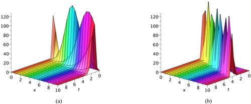
It is worth mentioning that the solutions obtained in this study represent certain real-life situations. For example, the tan-hyperbolic solutions are useful in calculating the magnetic moment and rapidity of special relativity, cos-hyperbolic solutions represent the shape of hanging cable, cot-hyperbolic solutions appear in the Langevin function which arise in magnetic polarization, sec-hyperbolic solutions represent the laminar jet profile [41]. Similarly, exact solutions with the periodic functions exhibit periodic wave phenomena. It is significant to mention here that a lot of new solutions have been produced for Murnaghan’s rod, and for the first time this equation has been solved for space–time fractional order. The reason of using fractional differential equation is that it is naturally related to physical phenomena with memory. Many well-known equations can be solved by space–time fractional differential equations to get variety of new solutions. For the better understanding of the solitary wave phenomenon graphs of some obtained solutions has been discussed here with the aid of mathematical software Maple 17. Figure 1 represents 3D graphs of $U_{1,1}$ which is dark soliton generated by taking fractional order $\alpha =0.7,1$, with some given parameters $p=3,q=1,r=2,b=0.5,\text{β}=1,E=4,ϵ=0.1,l=2,\upsilon =2,\delta =6$. Figure 2 represents 3D graphs of solutions $U_{1,20}$ with fractional order $\alpha =0.6,1$, exhibits combined singular periodic wave solution by taking parameters $p=5,q=2,r=1,b=0.3,\text{β}=1.5,E=10,ϵ=0.5,l=2,\upsilon =3.5,\delta =22.5$. Figure 3 represents 3D graphs dark singular solitons of $U_{2,5}$ with fractional order $\alpha =0.6,1$ by choosing parameters $p=5,q=2,r=1,b=0.3,\text{β}=1.5,E=10,ϵ=0.5,l=2,\upsilon =3.5,\delta =\mathrm{22.5.}$ Figure 4 represents 3D graphs of combined dark-bright soliton generated by $U_{3,3}$ with fractional order $\alpha =0.4,1$, by taking $p=3,q=2,r=1,b=0.3,\text{β}=1.5,E=10,ϵ=0.5,l=2,\upsilon =3.5,\delta =22.5$. Figure 5 represents 3D graphs of solitary wave solution $U_{4,6}$ with fractional order $\alpha =0.5,1$ with parameters $p=5,q=3,r=1,b=0.9,\text{β}=5,E=11,ϵ=0.05,l=2,\upsilon =5,\delta =33,A=2,B=3.$

Figure 1. 3D graphs of solitary wave solution $U_{1,1}$ with fractional order $\alpha =0.7,1$_.

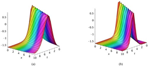
Figure 2. 3D graphs of periodic wave solution $U_{1,20}$ with fractional order $\alpha =0.6,1$_.

Figure 3. 3D graphs of solitary wave solution $U_{2,5}$ with fractional order $\alpha =0.6,1$_.

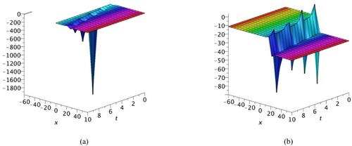
Figure 4. 3D graphs of solitary wave solution $U_{3,3}$ with fractional order $\alpha =0.4,1$_.

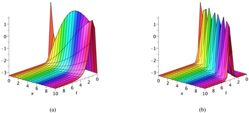
Figure 5. 3D graphs of solitary wave solution $U_{4,6}$ with fractional order $\alpha =0.5,1$_.

6. Conclusion

In this paper, improved generalized Riccati equation mapping method has been successfully applied to secure new and more general solutions to the space–time fractional Murnaghan’s rod equation. As a result, some totally new solutions have been obtained including several solitary wave solutions: dark, combined dark-bright, singular periodic wave, combined singular periodic wave solutions and one rational solution. These new solutions might be very useful in the study of seismology, physical properties of brass, steel and new elastic materials like polymers. The obtained results show that this mathematical technique is very effective and to find more general solutions of many NPDEs arising in plasma physics, mathematical physics, chemistry, many engineering disciplines and in natural sciences. The physical interpretation of these solutions has been highlighted with the help of 3D graphs and all the solutions obtained in this article have been verified by back substitution in original equation by using Maple 17.

Disclosure statement

No potential conflict of interest was reported by the authors.

References

- K. Diethelm, The analysis of fractional differential equations: An application-oriented exposition using differential operators of caputo type. Berlin: Springer-Verlag, 2010.
- Iqbal M, seadawy AR, Lu D. Construction of solitary wave solutions to the nonlinear modified Kortewege-de Vries dynamical equation in unmagnetized plasma via mathematical methods. Mod Phys Lett A. 2018;33(32):1850183.
- Lu D, Seadawy AR, Iqbal M. Mathematical methods via construction of traveling and solitary wave solutions of three coupled system of nonlinear partial differential equations and their applications. Results Phys. 2018;11:1161–1171.
- Iqbal M, Seadawy AR, Lu D, et al. Construction of a weakly nonlinear dispersion solitary wave solution for the Zakharov–Kuznetsov-modified equal width dynamical equation. Indian J Phys. 2020;94:1465–1474.
- Seadawy AR, Iqbal M, Lu D. Propagation of kink and anti-kink wave solitons for the nonlinear damped modified Korteweg–de Vries equation arising in ion-acoustic wave in an unmagnetized collisional dusty plasma. Physica A. 2020;544:123560.
- Iqbal M, Seadawy AR, Lu D. Dispersive solitary wave solutions of nonlinear further modified Korteweg–de Vries dynamical equation in an unmagnetized dusty plasma. Mod Phys Lett A. 2018;33(37):1850217.
- Iqbal M, Seadawy AR, Lu D. Applications of nonlinear longitudinal wave equation in a magneto-electro-elastic circular rod and new solitary wave solutions. Mod Phys Lett B. 2019;33(18):1950210.
- Seadawy AR, Iqbal M, Lu D. Applications of propagation of long-wave with dissipation and dispersion in nonlinear media via solitary wave solutions of generalized Kadomtsev–Petviashvili modified equal width dynamical equation. Comput Math Appl. 2019;78(11):3620–3632.
- Seadawy AR, Iqbal M, Lu D. Propagation of long-wave with dissipation and dispersion in nonlinear media via generalized Kadomtsive–Petviashvili modified equal width-Burgers equation. Indian J Phys. 2020;94(5):675–687.
- Iqbal M, Seadawy AR, Lu D, et al. Construction of bright–dark solitons and ion-acoustic solitary wave solutions of dynamical system of nonlinear wave propagation. Mod Phys Lett A. 2019;34(37):1950309.
- Seadawy AR, Iqbal M, Lu D. Construction of soliton solutions of the modify unstable nonlinear Schrödinger dynamical equation in fiber optics. Indian J Phys. 2020;94:823–832.
- Seadawy AR, Iqbal M, Lu D. Nonlinear wave solutions of the Kudryashov–Sinelshchikov dynamical equation in mixtures liquid-gas bubbles under the consideration of heat transfer and viscosity. J Taibah Univ Sci. 2019;13(1):1060–1072.
- Iqbal M, Seadawy AR, Khalil OH, et al. Propagation of long internal waves in density stratified ocean for the (2+1)-dimensional nonlinear Nizhnik–Novikov–Vesselov dynamical equation. Results hys. 2020;16:102838.
- Mohyud-Din ST, Noor MA. Homotopy perturbation method for solving partial differential equations. Z Naturforsch A. 2009;64(3–4):157–170.
- Shang Y. A lie algebra approach to susceptible-infected-susceptible epidemics. Electron J Differ Equ. 2012;2012:1–7.
- Shang Y. Lie algebraic discussion for affinity based information diffusion in social networks. Open Phys. 2017;15(1):705–711.
- Sakar MG, Ergören H. Alternative variational iteration method for solving the time-fractional Fornberg–whitham equation. Appl Math Model. 2015;39(14):3972–3979.
- Abdou M, Soliman A. New applications of variational iteration method. Physica D. 2005;211(1):1–8.
- Zhang S, Xia T. An improved generalized F-expansion method and its application to the (2+1)-dimensional KdV equations. Commun Nonlinear Sci Numer Simul. 2008;13(7):1294–1301.
- Navickas Z, Ragulskis M, Listopadskis N, et al. Comments on ‘soliton solutions to fractional-order nonlinear differential equations based on the exp-function method’. Optik. 2017;132:223–231.
- Navickas Z, Telksnys T, Ragulskis M. Comments on ‘The exp-function method and generalized solitary solutions’. Comput Math Appl. 2015;69(8):798–803.
- Zhang S, Xia TC. A further improved extended Fan sub-equation method and its application to the (3+1)-dimensional Kadomstev–Petviashvili equation. Phys Lett A. 2006;356(2):119–123.
- Guner O, Atik H, Kayyrzhanovich AA. New exact solution for space–time fractional differential equations via (G′/G)-expansion method. Optik. 2017;130:696–701.
- Manafian J, Lakestani M. Application of tan(ϕ/2)-expansion method for solving the Biswas–Milovic equation for Kerr law nonlinearity. Optik. 2016;127(4):2040–2054.
- Akbulut A, Kaplan M, Tascan F. The investigation of exact solutions of nonlinear partial differential equations by using exp(−Φ(ξ)) method. Optik. 2017;132:382–387.
- Kudryashov NA. One method for finding exact solutions of nonlinear differential equations. Commun Nonlinear Sci Numer Simul. 2012;17(6):2248–2253.
- Zhu S. The generalizing Riccati equation mapping method in non-linear evolution equation: application to (2+1)-dimensional Boiti–Leon–Pempinelle equation. Chaos Solitons Fractals. 2008;37(5):1335–1342.
- Bekir A, Cevikel AC. The tanh–coth method combined with the Riccati equation for solving nonlinear coupled equation in mathematical physics. J King Saud Univ - Sci. 2011;23(2):127–132.
- Li B, Chen Y, Xuan H, et al. Generalized Riccati equation expansion method and its application to the (3+1)-dimensional Jumbo–Miwa equation. Appl Math Comput. 2004;152(2):581–595.
- Tala-Tebue E, Tsobgni-Fozap DC, Kenfack-Jiotsa A, et al. Envelope periodic solutions for a discrete network with the Jacobi elliptic functions and the alternative (G′/G)-expansion method including the generalized Riccati equation. Eur Phys J Plus. 2014;129(6):136.
- Salathiel Y, Amadou Y, Betchewe G, et al. Soliton solutions and traveling wave solutions for a discrete electrical lattice with nonlinear dispersion through the generalized Riccati equation mapping method. Nonlinear Dyn. 2017;87(4):2435–2443.
- Koonprasert S, Sirisubtawee S, Ampun S. More explicit solitary solutions of the space-time fractional fifth order nonlinear Sawada–Kotera equation via the improved generalized Riccati equation mapping method. 2017.
- Bibi S, Ahmed N, Faisal I, et al. Some new solutions of the Caudrey–Dodd–Gibbon (CDG) equation using the conformable derivative. Adv Differ Equ. 2019;2019(1):89.
- Samsonov A. Strain solitons in solids and how to construct them. Boca Raton (FL): Chapman and Hall/CRC; Dec 18, 2020.
- Erbay HA, Erbay S, Erkip A. Thresholds for global existence and blow-up in a general class of doubly dispersive nonlocal wave equations. Nonlinear Anal: Theory Methods Appl. 2014;95:313–322.
- Cattani C, Sulaiman TA, Baskonus HM, et al. Solitons in an inhomogeneous Murnaghan’s rod. Eur Phys J Plus. 2018;133(6):228.
- Silambarasan R, Baskonus HM, Bulut H. Jacobi elliptic function solutions of the double dispersive equation in the Murnaghan’s rod. Eur Phys J Plus. 2019;134(3):125.
- I. Podlubny, Fractional differential equations: An introduction to fractional derivatives, fractional differential equations, to methods of their solution and some of their applications. Slovak Republic: Academic Press, 1999.
- He J-H, Elagan SK, Li ZB. Geometrical explanation of the fractional complex transform and derivative chain rule for fractional calculus. Phys Lett A. 2012;376(4):257–259.
- Guner O, Bekir A. On the concept of exact solution for nonlinear differential equations of fractional-order. Math Methods Appl Sci. 2016;39(14):4035–4043.
- Abbott S, Weisstein EW. CRC concise encyclopedia of mathematics. Math Gazette. 2007;84(501):549.