Numerical solution of a critical Sobolev exponent problem with weight on 𝕊³

Abstract

In this paper, we prove the existence of a positive solution for elliptic nonlinear partial differential equation with weight involving a critical exponent of Sobolev imbedding on ${\mathbb{S}}^3$. Moreover, we discuss numerically the influence of the weight on the radius of the domain for which the given PDE has a positive solution.

Keywords:

• Critical Sobolev exponent
• variational methods
• Runge–Kutta method

2010 Mathematics Subject Classifications:

• 35J20
• 35J25
• 35H30
• 35J60
• 65L06

1. Introduction

Let D be a geodesic ball with radius ${\theta }_1$, centred at the north pole, on ${\mathbb{S}}^3$. We study the following elliptic nonlinear partial differential equation with weight involving the critical exponent of Sobolev imbedding on ${\mathbb{S}}^3$ (1) $\{\begin{array}{ll}{\displaystyle -{\mathrm{div}}_{{\mathbb{S}}^3}((\alpha +\beta |x{|}^k){\mathrm{\nabla }}_{{\mathbb{S}}^3}u)=u^5+\lambda u,}& \mathrm{in}D,\\ u>0& \\ {\displaystyle u=0}& \mathrm{on}\mathrm{\partial }D,\end{array}$(1) where the exponent 5 + 1 = 6 is critical in the sense of Sobolev embedding, and the constants α, k, β and the parameter λ are assumed to be positive.

The partial differential equations are one of the most celebrate tools discovered from modelling many phenomena in nature. The differential equation in (1(1) $\{\begin{array}{ll}{\displaystyle -{\mathrm{div}}_{{\mathbb{S}}^3}((\alpha +\beta |x{|}^k){\mathrm{\nabla }}_{{\mathbb{S}}^3}u)=u^5+\lambda u,}& \mathrm{in}D,\\ u>0& \\ {\displaystyle u=0}& \mathrm{on}\mathrm{\partial }D,\end{array}$(1) ) can be a laboratory of finding many methods to deal with similar mathematical models which arise in different branch of sciences [1–17]. The problem (1(1) $\{\begin{array}{ll}{\displaystyle -{\mathrm{div}}_{{\mathbb{S}}^3}((\alpha +\beta |x{|}^k){\mathrm{\nabla }}_{{\mathbb{S}}^3}u)=u^5+\lambda u,}& \mathrm{in}D,\\ u>0& \\ {\displaystyle u=0}& \mathrm{on}\mathrm{\partial }D,\end{array}$(1) ) is interesting to study and has different new features, since this model is the stationary equation of convection–diffusion models appearing frequently in connection with conservation laws. The proposed problem has also some connections with non-stationary equations [1–3]. More precisely, for example in [3], Md N. Alam and C. Tunç use the modified $(G^{\prime }/G)$-expansion process to obtain soliton answers of the $(3+1)$ dimensional conformable fraction Zakharov–Kuznetsov equation with power law nonlinearity ${\displaystyle \frac{{\mathrm{\partial }}^{\alpha }u}{\mathrm{\partial }{t}^{\alpha }}+a{u}^n\frac{\mathrm{\partial }u}{\mathrm{\partial }x}+b\frac{\mathrm{\partial }}{\mathrm{\partial }x}(\frac{{\mathrm{\partial }}^{2}u}{\mathrm{\partial }{x}^2}+\frac{{\mathrm{\partial }}^{2}u}{\mathrm{\partial }{y}^2}+\frac{{\mathrm{\partial }}^{2}u}{\mathrm{\partial }{z}^2})=0}$. The authors apply some change of variables, namely $u=u(\xi )=u(x,y,z,t)$ with $\xi =x+y+z-V\frac{t^{\alpha }}{\alpha }$. They obtained the following equation ${\displaystyle 3b\frac{{\mathrm{\partial }}^{2}u}{\mathrm{\partial }{\xi }^2}-Vu+\frac{a}{n+1}{u}^{n+1}=0}$ which correspond to our problem when $\beta =0$.

On ${\mathbb{S}}^3$, Bandle and Benguria [4] investigated the problem (1(1) $\{\begin{array}{ll}{\displaystyle -{\mathrm{div}}_{{\mathbb{S}}^3}((\alpha +\beta |x{|}^k){\mathrm{\nabla }}_{{\mathbb{S}}^3}u)=u^5+\lambda u,}& \mathrm{in}D,\\ u>0& \\ {\displaystyle u=0}& \mathrm{on}\mathrm{\partial }D,\end{array}$(1) ) with $\alpha =1$ and $\beta =0$. In a bounded domain of $R^N$, Brezis and Nirenberg [10] treated the case $\alpha =1$ and $\beta =0$. The general case $\alpha \ne 0$ and $\beta \ne 0$ was studied by Hadiji and Yazidi in [15].

In this work, we treat the general case of α and β in a bounded domain of ${\mathbb{S}}^3$. More precisely, we study the influence of the function $\alpha +\beta |x{|}^k$ on the existence of solutions of a weighted elliptic PDE. Our method combined two directions: first, we study the existence of a positive solution. This procedure is not obvious and presents many difficulties due to the presence of critical Sobolev exponent which generate a lack of compactness. We overcome this problem using minimizing technique and variational approach. We obtain the existence of a positive solution only in the case k>1 and for λ in a well-determined interval. Therefore, second, in order to obtain a complete result of our problem, we use Newton iteration method with classical fourth-order Runge–Kutta procedure and we carry out a numerical solution in the cases that we have no theoretical results.

Using the stereographic transformation, D is mapped onto a ball $B(0,R)\subset {\mathbb{R}}^3$ and we write (1(1) $\{\begin{array}{ll}{\displaystyle -{\mathrm{div}}_{{\mathbb{S}}^3}((\alpha +\beta |x{|}^k){\mathrm{\nabla }}_{{\mathbb{S}}^3}u)=u^5+\lambda u,}& \mathrm{in}D,\\ u>0& \\ {\displaystyle u=0}& \mathrm{on}\mathrm{\partial }D,\end{array}$(1) ) as (2) $\{\begin{array}{ll}{\displaystyle -\mathrm{div}(\rho (x)(\alpha +\beta |x{|}^k)\mathrm{\nabla }u)={\rho }^3(x)u^5}& \mathrm{in}B(0,R),\\ +\lambda {\rho }^3(x)u,u>0& \\ {\displaystyle u=0}& \mathrm{on}\mathrm{\partial }B(0,R),\end{array}$(2) where $\rho (x)=\frac{2}{1+|x{|}^2}$.

By a result of Padilla [16] (extending the classical result of Gidas, Ni and Nirenberg [13] to domain on manifolds of constant curvature), a solution u of (2(2) $\{\begin{array}{ll}{\displaystyle -\mathrm{div}(\rho (x)(\alpha +\beta |x{|}^k)\mathrm{\nabla }u)={\rho }^3(x)u^5}& \mathrm{in}B(0,R),\\ +\lambda {\rho }^3(x)u,u>0& \\ {\displaystyle u=0}& \mathrm{on}\mathrm{\partial }B(0,R),\end{array}$(2) ) is symmetric, i.e. it only depends on the azimuthal angle, then we write (2(2) $\{\begin{array}{ll}{\displaystyle -\mathrm{div}(\rho (x)(\alpha +\beta |x{|}^k)\mathrm{\nabla }u)={\rho }^3(x)u^5}& \mathrm{in}B(0,R),\\ +\lambda {\rho }^3(x)u,u>0& \\ {\displaystyle u=0}& \mathrm{on}\mathrm{\partial }B(0,R),\end{array}$(2) ) as the boundary problem (3) $\{\begin{array}{ll}{\displaystyle -\mathrm{div}(\rho (r)r^2(\alpha +\beta r^k)\mathrm{\nabla }u)={\rho }^3(r)r^2{u}^5}& \mathrm{in}(0,R),\\ +\lambda {\rho }^3(r)r^{2}u,& \\ {\displaystyle u(R)=0\mathrm{and}{u}^{\prime }(0)=0,}\end{array}$(3) with $\rho (r)=\frac{2}{1+r^2}$.

For large dimensions $N\ge 5$, there is a little difference between studying the problem for a domain in ${\mathbb{S}}^N$ and a domain in ${\mathbb{R}}^N$. However, the results differ considerably for N = 4 and N = 3, see [4] for $S^3$ and [10] for ${\mathbb{R}}^N$. So, in this work we will study the case N = 3 where we prove the existence of a positive solution for $\lambda >0$ and k>1. We have no theoretical results for $\lambda >0$ and $0<k\le 1$ or $\lambda <0$ and k>1. Nevertheless, we obtain some numerical results for the existence of a positive solution. This approach is motivated by the results of [4] and [7] for $\alpha =1$ and $\beta =0$, where the authors found numerical solutions for λ negative enough when the geodesic radius ${\theta }_1>\frac{\pi }{2}$.

The rest of the paper is organized as follows: in Section 2, we present some theoretical results. In Section 3, we present numerical results for existence that complete the results announced in Section 2. Furthermore, in Section 4 we give some interpretations on the influence of the parameters k, α, β and λ, in a ball with radius R where the problem has a positive solution. Finally, in Section 5 we summarize our results and describe future work.

2. Theoretical results

Let ${\lambda }_1^{div}$ be the first eigenvalue of $-{\mathrm{div}}_{S^3}((\alpha +\beta |x{|}^k){\mathrm{\nabla }}_{S^3}u)$ on D with zero Dirichlet boundary condition.

We define $\gamma (\phi )=\frac{\begin{array}{c}{\int }_0^R(\alpha +\beta r^k)\rho (r)({\phi }^{\prime }(r){)}^2\mathrm{d}r+\beta {\int }_0^R\rho (r)(\phi (r){)}^2\\ r^{k-2}\mathrm{d}r-{\int }_0^R(\alpha +\beta r^k)(\rho (r){)}^2(\phi (r){)}^2\mathrm{d}r\end{array}}{{\int }_0^R(\rho (r){)}^3(\phi (r){)}^2\mathrm{d}r},$and (4) $\begin{array}{rl}{\lambda }^{\ast }(k)& =inf\{\gamma (\phi ),\phi \in C_0^{\mathrm{\infty }}(B(0,R))\phi \equiv 1\mathrm{in}B(0,R/4),\\ & \phantom{\{\gamma (\phi ),\phi \in C_0^{\mathrm{\infty }}(B(0,R))\phi \equiv 1\mathrm{in}B(0,R/4),}\phi \equiv 0\mathrm{on}B(0,R)\setminus B(0,R/3)\}.\end{array}$(4) The main result is:

Theorem 2.1

(1)	For k>1 there exists a positive solution of the Equation (3(3) $\{\begin{array}{ll}{\displaystyle -\mathrm{div}(\rho (r)r^2(\alpha +\beta r^k)\mathrm{\nabla }u)={\rho }^3(r)r^2{u}^5}& \mathrm{in}(0,R),\\ +\lambda {\rho }^3(r)r^{2}u,& \\ {\displaystyle u(R)=0\mathrm{and}{u}^{\prime }(0)=0,}\end{array}$(3) ) for $\lambda \in ({\lambda }^{\ast }(k),{\lambda }_1^{div})$.
(2)	There is no solution of (3(3) $\{\begin{array}{ll}{\displaystyle -\mathrm{div}(\rho (r)r^2(\alpha +\beta r^k)\mathrm{\nabla }u)={\rho }^3(r)r^2{u}^5}& \mathrm{in}(0,R),\\ +\lambda {\rho }^3(r)r^{2}u,& \\ {\displaystyle u(R)=0\mathrm{and}{u}^{\prime }(0)=0,}\end{array}$(3) ) for $\lambda \ge {\lambda }_1^{div}$

Let S be the best Sobolev constant for the injection of $H_0^1(D)$ into $L^6(D)$. We consider the associate minimizing problem to (2(2) $\{\begin{array}{ll}{\displaystyle -\mathrm{div}(\rho (x)(\alpha +\beta |x{|}^k)\mathrm{\nabla }u)={\rho }^3(x)u^5}& \mathrm{in}B(0,R),\\ +\lambda {\rho }^3(x)u,u>0& \\ {\displaystyle u=0}& \mathrm{on}\mathrm{\partial }B(0,R),\end{array}$(2) ) (5) $\begin{array}{rl}{S}_{\lambda ,\alpha ,\beta }& =\underset{u\in H_0^1(D)\setminus \{0\}}{inf}\\ & \times \left\{\frac{\begin{array}{c}{\int }_D(\alpha +\beta |x{|}^k)\rho (x)|\mathrm{\nabla }u{|}^2\mathrm{d}x\\ -\lambda {\int }_D(\rho (x){)}^3|u{|}^2\mathrm{d}x\end{array}}{{({\int }_D(\rho (x){)}^3|u{|}^6)}^{\frac{1}{3}}}\right\}.\end{array}$(5) The proof of the first part of Theorem 2.1 is based on the two following lemmas.

Lemma 2.1

If $S_{\lambda ,\alpha ,\beta }<\alpha S$, then the problem (5(5) $\begin{array}{rl}{S}_{\lambda ,\alpha ,\beta }& =\underset{u\in H_0^1(D)\setminus \{0\}}{inf}\\ & \times \left\{\frac{\begin{array}{c}{\int }_D(\alpha +\beta |x{|}^k)\rho (x)|\mathrm{\nabla }u{|}^2\mathrm{d}x\\ -\lambda {\int }_D(\rho (x){)}^3|u{|}^2\mathrm{d}x\end{array}}{{({\int }_D(\rho (x){)}^3|u{|}^6)}^{\frac{1}{3}}}\right\}.\end{array}$(5) ) has a minimizer.

Proof.

See Lemma 1.1 in [10] and Lemma 3.1 in [15].

Lemma 2.2

We have (6) $S_{\lambda ,\alpha ,\beta }\{\begin{array}{l}{\displaystyle <\alpha S,\mathrm{if}k>1}\\ {\displaystyle \le \alpha S,\mathrm{if}k\le 1.}\end{array}$(6)

Proof.

We define $Q_{\lambda ,k}(u)=\frac{{\int }_{D}q(x)\rho (x)|\mathrm{\nabla }u{|}^2\mathrm{d}x-\lambda {\int }_D(\rho (x){)}^3|u{|}^2\mathrm{d}x}{{({\int }_D(\rho (x){)}^3|u{|}^6)}^{\frac{1}{3}}},$with $q(x)=q(r)=\alpha +\beta |x{|}^k$ with $r=|x|$.

Next, we estimate the energy at $u_{\epsilon }(r)=\frac{{\epsilon }^{\frac{1}{4}}\phi (r)}{(\epsilon +r^2{)}^{\frac{1}{2}}}$. Using (16) and (24) in [4] and [15], we have (7) $\begin{array}{rl}& {\int }_0^R{u}_{\epsilon }^2{\rho }^3{r}^2\mathrm{d}r=4\pi {\epsilon }^{\frac{1}{2}}{\int }_0^R(\phi (r){)}^2(\rho (r){)}^3\mathrm{d}r+o({\epsilon }^{\frac{1}{2}}),\end{array}$(7) (8) $\begin{array}{rl}& {\left({\int }_0^R{u}_{\epsilon }^{2^{\ast }}{\rho }^3{r}^2\mathrm{d}r\right)}^{\frac{1}{3}}=(2{\pi }^2{)}^{\frac{1}{3}}+O(\epsilon ),\end{array}$(8) and

(9) $\begin{array}{rl}& {\displaystyle {\int }_0^{R}q(r){{\displaystyle \frac{\mathrm{\partial }{u}_{\epsilon }}{\mathrm{\partial }r}}}^2\rho r^2\mathrm{d}r=24\alpha {\int }_0^{\mathrm{\infty }}\frac{t^2}{(1+t^2{)}^3}\mathrm{d}t}\\ & {\displaystyle +\{\begin{array}{l}{\displaystyle 4\pi {\epsilon }^{\frac{1}{2}}[{\int }_0^{R}q(r)\rho (r)[({\phi }^{\prime }(r){)}^2-(\phi (r){)}^2]\mathrm{d}r}\\ {\displaystyle +\beta {\int }_0^R\rho (r)(\phi (r){)}^2{r}^{k-2}\mathrm{d}r]+o({\epsilon }^{{\displaystyle \frac{1}{2}}}),}& \mathrm{if}k>1,\\ {\displaystyle 8\pi 2\beta k{\epsilon }^{{\displaystyle \frac{1}{2}}}|\ln (\epsilon )|+o({\epsilon }^{{\displaystyle \frac{1}{2}}}|\ln (\epsilon )|),}& \mathrm{if}k=1,\\ {\displaystyle 8\pi \beta {\epsilon }^{\frac{k}{2}}[k{\int }_0^{\mathrm{\infty }}\frac{t^{k+2}}{(1+t^2{)}^3}\mathrm{d}t}\\ {\displaystyle +3{\int }_0^{\mathrm{\infty }}\frac{t^{k+2}}{(1+t^2{)}^3}\mathrm{d}t]+o({\epsilon }^{\frac{k}{2}}),}& \mathrm{if}k<1.\end{array}}\end{array}$(9) Combining (7(7) $\begin{array}{rl}& {\int }_0^R{u}_{\epsilon }^2{\rho }^3{r}^2\mathrm{d}r=4\pi {\epsilon }^{\frac{1}{2}}{\int }_0^R(\phi (r){)}^2(\rho (r){)}^3\mathrm{d}r+o({\epsilon }^{\frac{1}{2}}),\end{array}$(7) ), (8(8) $\begin{array}{rl}& {\left({\int }_0^R{u}_{\epsilon }^{2^{\ast }}{\rho }^3{r}^2\mathrm{d}r\right)}^{\frac{1}{3}}=(2{\pi }^2{)}^{\frac{1}{3}}+O(\epsilon ),\end{array}$(8) ) and (9(9) $\begin{array}{rl}& {\displaystyle {\int }_0^{R}q(r){{\displaystyle \frac{\mathrm{\partial }{u}_{\epsilon }}{\mathrm{\partial }r}}}^2\rho r^2\mathrm{d}r=24\alpha {\int }_0^{\mathrm{\infty }}\frac{t^2}{(1+t^2{)}^3}\mathrm{d}t}\\ & {\displaystyle +\{\begin{array}{l}{\displaystyle 4\pi {\epsilon }^{\frac{1}{2}}[{\int }_0^{R}q(r)\rho (r)[({\phi }^{\prime }(r){)}^2-(\phi (r){)}^2]\mathrm{d}r}\\ {\displaystyle +\beta {\int }_0^R\rho (r)(\phi (r){)}^2{r}^{k-2}\mathrm{d}r]+o({\epsilon }^{{\displaystyle \frac{1}{2}}}),}& \mathrm{if}k>1,\\ {\displaystyle 8\pi 2\beta k{\epsilon }^{{\displaystyle \frac{1}{2}}}|\ln (\epsilon )|+o({\epsilon }^{{\displaystyle \frac{1}{2}}}|\ln (\epsilon )|),}& \mathrm{if}k=1,\\ {\displaystyle 8\pi \beta {\epsilon }^{\frac{k}{2}}[k{\int }_0^{\mathrm{\infty }}\frac{t^{k+2}}{(1+t^2{)}^3}\mathrm{d}t}\\ {\displaystyle +3{\int }_0^{\mathrm{\infty }}\frac{t^{k+2}}{(1+t^2{)}^3}\mathrm{d}t]+o({\epsilon }^{\frac{k}{2}}),}& \mathrm{if}k<1.\end{array}}\end{array}$(9) ) we get

(10) $\begin{array}{rl}& {\displaystyle Q_{q,\lambda }(u_{\epsilon })=\alpha S+(2^5\pi {)}^{\frac{1}{3}}}\\ & \times \{\begin{array}{l}{\displaystyle {\epsilon }^{\frac{1}{2}}[{\int }_0^{R}q(r)\rho (r)[({\phi }^{\prime }(r){)}^2-(\phi (r){)}^2]\mathrm{d}r}\\ {\displaystyle +\beta {\int }_0^R\rho (r)(\phi (r){)}^2{r}^{k-2}\mathrm{d}r]}\\ {\displaystyle -\lambda {\epsilon }^{\frac{1}{2}}{\int }_0^R(\rho (r){)}^3(\phi (r){)}^2\mathrm{d}r+o({\epsilon }^{\frac{1}{2}}),}& \mathrm{if}k>1,\\ {\displaystyle 2\beta k{\epsilon }^{{\displaystyle \frac{1}{2}}}|\ln (\epsilon )|+o({\epsilon }^{\frac{1}{2}}|\ln (\epsilon )|),}& \mathrm{if}k=1,\\ {\displaystyle 2\beta {\epsilon }^{{\displaystyle \frac{k}{2}}}[k{\int }_0^{\mathrm{\infty }}{\displaystyle \frac{t^{k+2}}{(1+t^2{)}^2}}\mathrm{d}t}\\ {\displaystyle +3{\int }_0^{\mathrm{\infty }}\frac{t^{k+2}}{(1+t^2{)}^3}\mathrm{d}t]+o({\epsilon }^{\frac{k}{2}}),}& \mathrm{if}k<1.\end{array}\end{array}$(10) Therefore, we can deduce a conclusion just when k>1, more precisely we have (11) $\begin{array}{rl}{\displaystyle Q_{q,\lambda }(u_{\epsilon })}& =\alpha S\\ & +{\displaystyle (2^5\pi {)}^{\frac{1}{3}}{\epsilon }^{\frac{1}{2}}}\\ & \times \left[{\displaystyle \frac{\begin{array}{c}{\int }_0^{R}q(r)\rho (r)[({\phi }^{\prime }(r){)}^2-(\phi (r){)}^2]\mathrm{d}r\\ +\beta {\int }_0^R\rho (r)(\phi (r){)}^2{r}^{k-2}\mathrm{d}r\end{array}}{{\int }_0^R(\rho (r){)}^3(\phi (r){)}^2\mathrm{d}r}-\lambda }\right]\\ & \times {\int }_0^R(\rho (r){)}^3(\phi (r){)}^2\mathrm{d}r\\ & {\displaystyle +o({\epsilon }^{\frac{1}{2}}).}\end{array}$(11) Finally, from the definition of ${\lambda }^{\ast }(k)$ in (4(4) $\begin{array}{rl}{\lambda }^{\ast }(k)& =inf\{\gamma (\phi ),\phi \in C_0^{\mathrm{\infty }}(B(0,R))\phi \equiv 1\mathrm{in}B(0,R/4),\\ & \phantom{\{\gamma (\phi ),\phi \in C_0^{\mathrm{\infty }}(B(0,R))\phi \equiv 1\mathrm{in}B(0,R/4),}\phi \equiv 0\mathrm{on}B(0,R)\setminus B(0,R/3)\}.\end{array}$(4) ) and the fact that $q(r)=\alpha +\beta r^k$, we conclude that $S_{\lambda ,\alpha ,\beta }<\alpha S$ when $\lambda >{\lambda }^{\ast }(k)$ and k>1.

Proof

Proof of Theorem 2.1

1. Let $(u_j)$ be a minimizing sequence of $S_{\lambda ,\alpha ,\beta }$. More precisely, $\begin{array}{rl}& {\int }_D(\alpha +\beta |x{|}^k)\rho (x)|\mathrm{\nabla }{u}_j{|}^2\mathrm{d}x-\lambda {\int }_D(\rho (x){)}^3|u_j{|}^2\mathrm{d}x\\ & =S_{\lambda ,\alpha ,\beta }+0(1),\end{array}$and ${({\int }_D(\rho (x){)}^3|u_j{|}^6)}^{\frac{1}{3}}=1.$From Lemma 6(6) $S_{\lambda ,\alpha ,\beta }\{\begin{array}{l}{\displaystyle <\alpha S,\mathrm{if}k>1}\\ {\displaystyle \le \alpha S,\mathrm{if}k\le 1.}\end{array}$(6) , we know that $S_{\lambda ,\alpha ,\beta }<\alpha S$ for $\lambda >{\lambda }^{\ast }(k)$ and k>1. Thus we have a minimizing sequence of $S_{\lambda ,\alpha ,\beta }$ and $S_{\lambda ,\alpha ,\beta }<\alpha S$. Consequently, from Lemma 2.1, we deduce that $S_{\lambda ,\alpha ,\beta }$ is achieved by a function u such that $u_j\to u$ strongly in $H_0^1(\mathrm{\Omega })$ and $\begin{array}{r}{\int }_D(\alpha +\beta |x{|}^k)\rho (x)|\mathrm{\nabla }u{|}^2\mathrm{d}x-\lambda {\int }_D(\rho (x){)}^3|u{|}^2\mathrm{d}x\\ =S_{\lambda ,\alpha ,\beta }\mathrm{and}{({\int }_D(\rho (x){)}^3|u_j{|}^6)}^{\frac{1}{3}}=1.\end{array}$We may assume that $u\ge 0$ (otherwise we replace u by $|u|$). Since u is a minimizer of (5(5) $\begin{array}{rl}{S}_{\lambda ,\alpha ,\beta }& =\underset{u\in H_0^1(D)\setminus \{0\}}{inf}\\ & \times \left\{\frac{\begin{array}{c}{\int }_D(\alpha +\beta |x{|}^k)\rho (x)|\mathrm{\nabla }u{|}^2\mathrm{d}x\\ -\lambda {\int }_D(\rho (x){)}^3|u{|}^2\mathrm{d}x\end{array}}{{({\int }_D(\rho (x){)}^3|u{|}^6)}^{\frac{1}{3}}}\right\}.\end{array}$(5) ) then there exists a Lagrange multiplier $\mu \in \mathbb{R}$ such that $\begin{array}{rl}& -\mathrm{div}(\rho (x)(\alpha +\beta |x{|}^k)\mathrm{\nabla }u)-\lambda {\rho }^3(x)u\\ & =\mu {\rho }^3(x)u^5\mathrm{in}\mathrm{\Omega }.\end{array}$In fact $\mu =S_{\lambda ,\alpha ,\beta }$ and $S_{\lambda ,\alpha ,\beta }>0$ since $\lambda <{\lambda }_1^{div}$. Then u>0 on Ω by the strong maximum principle. Finally, there exists a positive constant k>0 (more precisely $k=(S_{\lambda ,\alpha ,\beta }{)}^{\frac{1}{4}}$ ) such that $ku$ is a solution of problem 2(2) $\{\begin{array}{ll}{\displaystyle -\mathrm{div}(\rho (x)(\alpha +\beta |x{|}^k)\mathrm{\nabla }u)={\rho }^3(x)u^5}& \mathrm{in}B(0,R),\\ +\lambda {\rho }^3(x)u,u>0& \\ {\displaystyle u=0}& \mathrm{on}\mathrm{\partial }B(0,R),\end{array}$(2) .

2. There is no solution of (2(2) $\{\begin{array}{ll}{\displaystyle -\mathrm{div}(\rho (x)(\alpha +\beta |x{|}^k)\mathrm{\nabla }u)={\rho }^3(x)u^5}& \mathrm{in}B(0,R),\\ +\lambda {\rho }^3(x)u,u>0& \\ {\displaystyle u=0}& \mathrm{on}\mathrm{\partial }B(0,R),\end{array}$(2) ) when $\lambda >{\lambda }_1^{div}$. Indeed, let ${\phi }_1$ be the eigenfunction of $-{\mathrm{div}}_{S^3}((\alpha +\beta |x{|}^k){\mathrm{\nabla }}_{S^3}u)$ corresponding to ${\lambda }_1^{div}$, with ${\phi }_1>0$ on D. More precisely, we have $-{\mathrm{div}}_{S^3}((\alpha +\beta |x{|}^k){\mathrm{\nabla }}_{S^3}{\phi }_1)={\lambda }_1^{div}{\phi }_1\mathrm{on}D,$equivalently, under the stereographic projection, to $\begin{array}{rl}& -\mathrm{div}(\rho (x)(\alpha +\beta |x{|}^k)\mathrm{\nabla }{\phi }_1)\\ & ={\lambda }_1^{div}{\rho }^3(x){\phi }_1\mathrm{on}B(0,R).\end{array}$Suppose that u is a solution of (2(2) $\{\begin{array}{ll}{\displaystyle -\mathrm{div}(\rho (x)(\alpha +\beta |x{|}^k)\mathrm{\nabla }u)={\rho }^3(x)u^5}& \mathrm{in}B(0,R),\\ +\lambda {\rho }^3(x)u,u>0& \\ {\displaystyle u=0}& \mathrm{on}\mathrm{\partial }B(0,R),\end{array}$(2) ), then we have $\begin{array}{rl}{\displaystyle {\lambda }_1^{div}{\int }_B{\rho }^{3}u{\phi }_1}& ={\int }_{\mathrm{\Omega }}-\mathrm{div}(\rho (\alpha +\beta |x{|}^k)\mathrm{\nabla }u){\phi }_1\\ & ={\displaystyle {\int }_B{\rho }^3{u}^5{\phi }_1+\lambda {\int }_B{\rho }^{3}u{\phi }_1}\\ & >{\displaystyle \lambda {\int }_{\mathrm{\Omega }}{\rho }^{3}u{\phi }_1.}\end{array}$Thus $\lambda <{\lambda }_1^{div}$, since the functions ρ, u and ${\phi }_1$ are positive which concludes the proof of Theorem 2.1.

3. Numerical study

From the boundary problem (3(3) $\{\begin{array}{ll}{\displaystyle -\mathrm{div}(\rho (r)r^2(\alpha +\beta r^k)\mathrm{\nabla }u)={\rho }^3(r)r^2{u}^5}& \mathrm{in}(0,R),\\ +\lambda {\rho }^3(r)r^{2}u,& \\ {\displaystyle u(R)=0\mathrm{and}{u}^{\prime }(0)=0,}\end{array}$(3) ), we have (12) $\{\begin{array}{l}{\displaystyle -{\left(\rho \left(r\right)p\left(r\right)r^2{u}^{\mathrm{\prime }}\left(r\right)\right)}^{{}^{\mathrm{\prime }}}=r^2{\rho }^2\left(r\right)u^5\left(r\right)}\\ +\lambda r^2{\rho }^3\left(r\right)u\left(r\right),\mathrm{for}r\in (0,R),\\ {\displaystyle u^{\mathrm{\prime }}(0)=u(R)=0,}\end{array}$(12) where $\rho (r)=\frac{2}{1+r^2},p(r)=\alpha +\beta r^k.$Let $u(r)=u(r;u_0)$ be a solution of the initial value problem (13) $\{\begin{array}{l}{\displaystyle -{\left(\rho \left(r\right)p\left(r\right)r^2{u}^{\mathrm{\prime }}\left(r\right)\right)}^{{}^{\mathrm{\prime }}}=r^2{\rho }^3\left(r\right)u^5\left(r\right)}\\ +\lambda r^2{\rho }^3\left(r\right)u\left(r\right),\mathrm{for}r\in (0,R),\\ {\displaystyle u^{\mathrm{\prime }}(0)=0,}\\ {\displaystyle u(0)=u_0>0,}\end{array}$(13) such that $u(R;u_0)=0.$Using Newton iteration method to approximate $u_0$: (14) $\begin{array}{rl}{u}_0^{j+1}& =u_0^j-{\left(\frac{\mathrm{\partial }}{\mathrm{\partial }{u}_0}u(R;u_0^j)\right)}^{-1}u(R;u_0^j),\\ & j=1,2,3,\dots ,n,\end{array}$(14) and differentiating the differential Equation (13(13) $\{\begin{array}{l}{\displaystyle -{\left(\rho \left(r\right)p\left(r\right)r^2{u}^{\mathrm{\prime }}\left(r\right)\right)}^{{}^{\mathrm{\prime }}}=r^2{\rho }^3\left(r\right)u^5\left(r\right)}\\ +\lambda r^2{\rho }^3\left(r\right)u\left(r\right),\mathrm{for}r\in (0,R),\\ {\displaystyle u^{\mathrm{\prime }}(0)=0,}\\ {\displaystyle u(0)=u_0>0,}\end{array}$(13) ) with respect to $u_0$, yields (15) $\{\begin{array}{l}{\displaystyle -{\left(\rho \left(r\right)p\left(r\right)r^2{v}^{\mathrm{\prime }}\left(r\right)\right)}^{{}^{\mathrm{\prime }}}=5r^2{\rho }^3\left(r\right)u^4\left(r\right)v\left(r\right)}\\ +\lambda r^2{\rho }^3\left(r\right)v\left(r\right),\mathrm{for}r\in (0,R),\\ {\displaystyle v^{\mathrm{\prime }}(0)=0,}\\ {\displaystyle v(0)=1,}\end{array}$(15) where $v\left(r\right)=\frac{\mathrm{\partial }}{\mathrm{\partial }{u}_0}u(R;u_0).$By substituting $\begin{array}{rl}x\left(r\right)& =r^2\rho \left(r\right)p\left(r\right)u^{\mathrm{\prime }}\left(r\right),\\ y\left(r\right)& =r^2\rho \left(r\right)p\left(r\right)v^{\mathrm{\prime }}\left(r\right),\end{array}$in Equations (13(13) $\{\begin{array}{l}{\displaystyle -{\left(\rho \left(r\right)p\left(r\right)r^2{u}^{\mathrm{\prime }}\left(r\right)\right)}^{{}^{\mathrm{\prime }}}=r^2{\rho }^3\left(r\right)u^5\left(r\right)}\\ +\lambda r^2{\rho }^3\left(r\right)u\left(r\right),\mathrm{for}r\in (0,R),\\ {\displaystyle u^{\mathrm{\prime }}(0)=0,}\\ {\displaystyle u(0)=u_0>0,}\end{array}$(13) ) and (15(15) $\{\begin{array}{l}{\displaystyle -{\left(\rho \left(r\right)p\left(r\right)r^2{v}^{\mathrm{\prime }}\left(r\right)\right)}^{{}^{\mathrm{\prime }}}=5r^2{\rho }^3\left(r\right)u^4\left(r\right)v\left(r\right)}\\ +\lambda r^2{\rho }^3\left(r\right)v\left(r\right),\mathrm{for}r\in (0,R),\\ {\displaystyle v^{\mathrm{\prime }}(0)=0,}\\ {\displaystyle v(0)=1,}\end{array}$(15) ), we get the following system of first-order differential equations: (16a) $\{\begin{array}{l}{\displaystyle u^{\mathrm{\prime }}\left(r\right)={\left(r^2\rho p\right)}^{-1}x,}\\ {\displaystyle x^{\mathrm{\prime }}\left(r\right)=-r^2{\rho }^3(u^5+\lambda u),}\\ {\displaystyle v^{\mathrm{\prime }}\left(r\right)={\left(r^2\rho p\right)}^{-1}y,}\\ {\displaystyle y^{\mathrm{\prime }}\left(r\right)=-r^2{\rho }^3(\lambda +(2^{\ast }-1)u^4)v,}\end{array}$(16a) subjected to the initial conditions (16b) $\{\begin{array}{c}{\displaystyle u\left(0\right)=u_0,}\\ {\displaystyle x\left(0\right)=0,}\\ {\displaystyle v\left(0\right)=1,}\\ {\displaystyle y\left(0\right)=0,}\end{array}$(16b) which can be written in a matrix form as ${\mathbf{w}}^{\mathrm{\prime }}=\mathbf{f}(r,\mathbf{w}),$with $\begin{array}{rl}\mathbf{w}& =\left(\begin{array}{c}u\\ x\\ v\\ y\end{array}\right)\mathrm{and}\\ \mathbf{f}(r,\mathbf{w})& =\left(\begin{array}{c}{\displaystyle {\left(r^2\rho p\right)}^{-1}x}\\ -r^2{\rho }^3(u^5+\lambda u)\\ {\displaystyle {\left(r^2\rho p\right)}^{-1}y}\\ -r^2{\rho }^3(\lambda +(2^{\ast }-1)u^4)v\end{array}\right).\end{array}$Using the classical fourth order Runge–Kutta method for the system (16a(16a) $\{\begin{array}{l}{\displaystyle u^{\mathrm{\prime }}\left(r\right)={\left(r^2\rho p\right)}^{-1}x,}\\ {\displaystyle x^{\mathrm{\prime }}\left(r\right)=-r^2{\rho }^3(u^5+\lambda u),}\\ {\displaystyle v^{\mathrm{\prime }}\left(r\right)={\left(r^2\rho p\right)}^{-1}y,}\\ {\displaystyle y^{\mathrm{\prime }}\left(r\right)=-r^2{\rho }^3(\lambda +(2^{\ast }-1)u^4)v,}\end{array}$(16a) )–(16b(16b) $\{\begin{array}{c}{\displaystyle u\left(0\right)=u_0,}\\ {\displaystyle x\left(0\right)=0,}\\ {\displaystyle v\left(0\right)=1,}\\ {\displaystyle y\left(0\right)=0,}\end{array}$(16b) ), and for a given step-size h>0 we define $\{\begin{array}{l}{\displaystyle {\mathbf{w}}_{i+1}={\mathbf{w}}_i+\frac{1}{6}}\\ ({\mathbf{k}}_1^i+2{\mathbf{k}}_2^i+2{\mathbf{k}}_3^i+{\mathbf{k}}_4^i)\\ {\displaystyle r_{i+1}=r_i+h}\end{array},\mathrm{for}i=0,1,2,3,\dots ,m,$where

$\begin{array}{rl}{\mathbf{k}}_1^i& =\mathbf{f}(r_i,{\mathbf{w}}_i)=h\left(\begin{array}{c}{\displaystyle {\left(r_i^2{\rho }_i{p}_i\right)}^{-1}{x}_i}\\ {\displaystyle -r_i^2{\rho }_i^3(u_i^5+\lambda u_i)}\\ {\displaystyle {\left(r_i^2{\rho }_i{p}_i\right)}^{-1}{y}_i}\\ {\displaystyle -r_i^2{\rho }_i^3(\lambda +(2^{\ast }-1)u_i^4)v_i}\end{array}\right),\\ {\mathbf{k}}_2^i& =h\left(\begin{array}{c}{\displaystyle {\left(r_{i+\frac{1}{2}}^2{\rho }_{i+\frac{1}{2}}{p}_{i+\frac{1}{2}}\right)}^{-1}(x_i+\frac{{\mathbf{k}}_{1,2}^i}{2})}\\ {\displaystyle -r_{i+\frac{1}{2}}^2{\rho }_{i+\frac{1}{2}}^3({(u_i+\frac{{\mathbf{k}}_{1,1}^i}{2})}^5+\lambda (u_i+\frac{{\mathbf{k}}_{1,1}^i}{2}))}\\ {\displaystyle {\left(r_{i+\frac{1}{2}}^2{\rho }_{i+\frac{1}{2}}{p}_{i+\frac{1}{2}}\right)}^{-1}(y_i+\frac{{\mathbf{k}}_{1,4}^i}{2})}\\ {\displaystyle -r_{i+\frac{1}{2}}^2{\rho }_{i+\frac{1}{2}}^3(\lambda +5{(u_i+\frac{{\mathbf{k}}_{1,1}^i}{2})}^4)(v_i+\frac{{\mathbf{k}}_{1,3}^i}{2})}\end{array}\right),\\ {\mathbf{k}}_3^i& =h\left(\begin{array}{c}{\displaystyle {\left(r_{i+\frac{1}{2}}^2{\rho }_{i+\frac{1}{2}}{p}_{i+\frac{1}{2}}\right)}^{-1}(x_i+\frac{{\mathbf{k}}_{2,2}^i}{2})}\\ {\displaystyle -r_{i+\frac{1}{2}}^2{\rho }_{i+\frac{1}{2}}^3({(u_i+\frac{{\mathbf{k}}_{2,1}^i}{2})}^5+\lambda (u_i+\frac{{\mathbf{k}}_{2,1}^i}{2}))}\\ {\displaystyle {\left(r_{i+\frac{1}{2}}^2{\rho }_{i+\frac{1}{2}}{p}_{i+\frac{1}{2}}\right)}^{-1}(y_i+\frac{{\mathbf{k}}_{2,4}^i}{2})}\\ {\displaystyle -r_{i+\frac{1}{2}}^2{\rho }_{i+\frac{1}{2}}^3(\lambda +5{(u_i+\frac{{\mathbf{k}}_{2,1}^i}{2})}^4)(v_i+\frac{{\mathbf{k}}_{2,3}^i}{2})}\end{array}\right),\\ {\mathbf{k}}_4^i& =h\left(\begin{array}{c}{\displaystyle {\left(r_{i+1}^2{\rho }_{i+1}{p}_{i+1}\right)}^{-1}(x_i+{\mathbf{k}}_{3,2}^i)}\\ {\displaystyle -r_{i+1}^2{\rho }_{i+1}^3({(u_i+{\mathbf{k}}_{3,1}^i)}^5+\lambda (u_i+{\mathbf{k}}_{3,1}^i))}\\ {\displaystyle {\left(r_{i+1}^2{\rho }_{i+1}{p}_{i+1}\right)}^{-1}(y_i+{\mathbf{k}}_{3,4}^i)}\\ {\displaystyle -r_{i+1}^2{\rho }_{i+1}^3(\lambda +(2^{\ast }-1){(u_i+{\mathbf{k}}_{3,1}^i)}^4)(v_i+{\mathbf{k}}_{3,3}^i)}\end{array}\right),\end{array}$which gives the solution $u_i=u_i(u_0)$ in terms of $u_0$ for $i=0,1,2,3,\dots ,m$, and the last nonlinear equation is (17) $u_m\left(u_0\right)=u\left(R\right)=0,$(17) and we have (18) $\left(\begin{array}{c}{u}_1\left(u_0\right)\\ u_2\left(u_0\right)\\ u_3\left(u_0\right)\\ ⋮\\ u_{m-1}\left(u_0\right)\\ u_m\left(u_0\right)=u\left(R\right)\end{array}\right).$(18) The last equation is nonlinear, which will be solved for $u_0$ by Newton iterative method: $\begin{array}{rl}{u}_0^{j+1}& =u_0^j-{(\frac{\mathrm{\partial }}{\mathrm{\partial }{u}_0}u(R;u_0^j))}^{-1}u(R;u_0^j),\\ & j=1,2,3,\dots ,n.\end{array}$Next, we solve the boundary value problem (12(12) $\{\begin{array}{l}{\displaystyle -{\left(\rho \left(r\right)p\left(r\right)r^2{u}^{\mathrm{\prime }}\left(r\right)\right)}^{{}^{\mathrm{\prime }}}=r^2{\rho }^2\left(r\right)u^5\left(r\right)}\\ +\lambda r^2{\rho }^3\left(r\right)u\left(r\right),\mathrm{for}r\in (0,R),\\ {\displaystyle u^{\mathrm{\prime }}(0)=u(R)=0,}\end{array}$(12) ) for different values of α, β, k, λ, and the corresponding R with the solutions are presented in Figures 1, 2, 3.

Figure 1. Numerical solutions of (12(12) $\{\begin{array}{l}{\displaystyle -{\left(\rho \left(r\right)p\left(r\right)r^2{u}^{\mathrm{\prime }}\left(r\right)\right)}^{{}^{\mathrm{\prime }}}=r^2{\rho }^2\left(r\right)u^5\left(r\right)}\\ +\lambda r^2{\rho }^3\left(r\right)u\left(r\right),\mathrm{for}r\in (0,R),\\ {\displaystyle u^{\mathrm{\prime }}(0)=u(R)=0,}\end{array}$(12) ) for $\alpha =1$, ${\beta }_k=1$, $\lambda =2$, and different values of R and k: (a) R = 0.981918, k = 0.1. (b) R = 1.08245, k = 0.5. (c) R = 1.08481, k = 0.9. (d) R = 1.07375, k = 1.

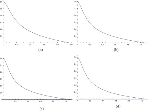
Figure 2. Numerical solutions of (12(12) $\{\begin{array}{l}{\displaystyle -{\left(\rho \left(r\right)p\left(r\right)r^2{u}^{\mathrm{\prime }}\left(r\right)\right)}^{{}^{\mathrm{\prime }}}=r^2{\rho }^2\left(r\right)u^5\left(r\right)}\\ +\lambda r^2{\rho }^3\left(r\right)u\left(r\right),\mathrm{for}r\in (0,R),\\ {\displaystyle u^{\mathrm{\prime }}(0)=u(R)=0,}\end{array}$(12) ) for $\alpha =1$, $\beta =1$, $\lambda =-6$, and different values of R and k: (a) R = 26.4421, k = 1.1. (b) R = 43.4183, k = 1.2. (c) R = 114.356, k = 1.3. (d) R = 316.708, k = 1.35.

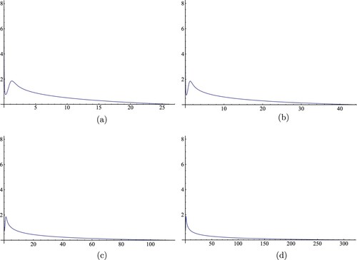
Figure 3. Numerical solutions of (12(12) $\{\begin{array}{l}{\displaystyle -{\left(\rho \left(r\right)p\left(r\right)r^2{u}^{\mathrm{\prime }}\left(r\right)\right)}^{{}^{\mathrm{\prime }}}=r^2{\rho }^2\left(r\right)u^5\left(r\right)}\\ +\lambda r^2{\rho }^3\left(r\right)u\left(r\right),\mathrm{for}r\in (0,R),\\ {\displaystyle u^{\mathrm{\prime }}(0)=u(R)=0,}\end{array}$(12) ) for $\lambda =6$ (a), (b) and $\lambda =-6$ (c), (d), with different values of R, k, α, β: (a) R = 1.89151, k = 0.9, $\alpha =2$, $\beta =5$; (b) R = 1.38993, k = 0.9, $\alpha =3$, $\beta =4$; (c) R = 29.3202, k = 1.1, $\alpha =0.5$, $\beta =0.25$; (d) R = 8.90831, k = 1.3, $\alpha =2$, $\beta =0.2$.

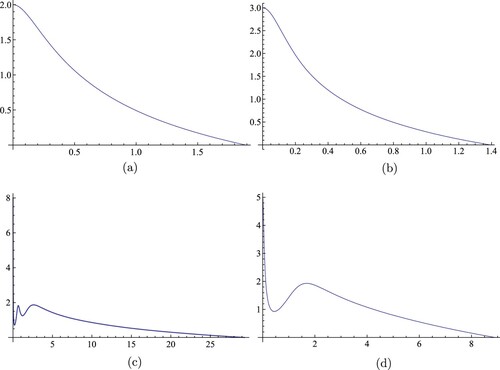
Figure 1 presents a numerical solution of (12(12) $\{\begin{array}{l}{\displaystyle -{\left(\rho \left(r\right)p\left(r\right)r^2{u}^{\mathrm{\prime }}\left(r\right)\right)}^{{}^{\mathrm{\prime }}}=r^2{\rho }^2\left(r\right)u^5\left(r\right)}\\ +\lambda r^2{\rho }^3\left(r\right)u\left(r\right),\mathrm{for}r\in (0,R),\\ {\displaystyle u^{\mathrm{\prime }}(0)=u(R)=0,}\end{array}$(12) ) in the case $\lambda >0$ and $0<k\le 1$, where $\alpha =1$, $\beta =1$, $\lambda =2$, and R = 0.981918, k = 0.1 (Figure 1 a), R = 1.08295, k = 0.5 (Figure 1 b), R = 1.08481, k = 0.9 (Figure 1 c), R = 1.08606, k = 1 (Figure 1 d). We notice that the numerical solution is decreasing from $u(0)$ to $u(R)=0$.

Next, Figure 2 gives a numerical solution of (12(12) $\{\begin{array}{l}{\displaystyle -{\left(\rho \left(r\right)p\left(r\right)r^2{u}^{\mathrm{\prime }}\left(r\right)\right)}^{{}^{\mathrm{\prime }}}=r^2{\rho }^2\left(r\right)u^5\left(r\right)}\\ +\lambda r^2{\rho }^3\left(r\right)u\left(r\right),\mathrm{for}r\in (0,R),\\ {\displaystyle u^{\mathrm{\prime }}(0)=u(R)=0,}\end{array}$(12) ) in the case $\lambda <0$ and k>1, where $\alpha =1$, $\beta =1$, $\lambda =-6$, and R = 26.4421, k = 1.1 (Figure 2 a), R = 43.4183, k = 1.2 (Figure 2 b), R = 114.356, k = 1.3 (Figure 2 c), R = 316.708, k = 1.35 (Figure 2 d). We observe that the numerical solution start by oscillating near the origin then decreases for a large value of the radius R to u(R) = 0.

Finally, Figure 3 illustrates a numerical solution of (12(12) $\{\begin{array}{l}{\displaystyle -{\left(\rho \left(r\right)p\left(r\right)r^2{u}^{\mathrm{\prime }}\left(r\right)\right)}^{{}^{\mathrm{\prime }}}=r^2{\rho }^2\left(r\right)u^5\left(r\right)}\\ +\lambda r^2{\rho }^3\left(r\right)u\left(r\right),\mathrm{for}r\in (0,R),\\ {\displaystyle u^{\mathrm{\prime }}(0)=u(R)=0,}\end{array}$(12) ) for $\alpha =2$, $\beta =5$, $\lambda =6$, R = 1.89151, k = 0.9 (Figure 3 a), $\alpha =3$, $\beta =4$, $\lambda =6$, R = 1.38993, k = 0.9 (Figure 3 b), $\alpha =0.5$, $\beta =0.25$, $\lambda =-6$, R = 29.3202, k = 1.1 (Figure 3 c), $\alpha =2$, $\beta =0.2$, $\lambda =-6$, R = 8.90831, k = 1.3 (Figure 3 d). We notice similar observations as in Figure 1 and Figure 2, respectively, for λ positive and negative.

4. Variation of the problem parameters

Next, for a given $u(0)=u_0>0$, we solve numerically the boundary value problem (12(12) $\{\begin{array}{l}{\displaystyle -{\left(\rho \left(r\right)p\left(r\right)r^2{u}^{\mathrm{\prime }}\left(r\right)\right)}^{{}^{\mathrm{\prime }}}=r^2{\rho }^2\left(r\right)u^5\left(r\right)}\\ +\lambda r^2{\rho }^3\left(r\right)u\left(r\right),\mathrm{for}r\in (0,R),\\ {\displaystyle u^{\mathrm{\prime }}(0)=u(R)=0,}\end{array}$(12) ) for different values of the parameters in both cases when λ positive and negative and choose the minimum radius R so that the obtained numerical solution stay positive.

• Case 1 ($\lambda >0$):

Example 4.1

We solve the boundary value problem (12(12) $\{\begin{array}{l}{\displaystyle -{\left(\rho \left(r\right)p\left(r\right)r^2{u}^{\mathrm{\prime }}\left(r\right)\right)}^{{}^{\mathrm{\prime }}}=r^2{\rho }^2\left(r\right)u^5\left(r\right)}\\ +\lambda r^2{\rho }^3\left(r\right)u\left(r\right),\mathrm{for}r\in (0,R),\\ {\displaystyle u^{\mathrm{\prime }}(0)=u(R)=0,}\end{array}$(12) ) for $\alpha =1$,k = 0.9, $\lambda =2$ with different values of β and the obtained minimum radius R satisfied the boundary condition $u(R)=0$ are presented in Table 1.

Table 1. Minimum radius R for (12(12) $\{\begin{array}{l}{\displaystyle -{\left(\rho \left(r\right)p\left(r\right)r^2{u}^{\mathrm{\prime }}\left(r\right)\right)}^{{}^{\mathrm{\prime }}}=r^2{\rho }^2\left(r\right)u^5\left(r\right)}\\ +\lambda r^2{\rho }^3\left(r\right)u\left(r\right),\mathrm{for}r\in (0,R),\\ {\displaystyle u^{\mathrm{\prime }}(0)=u(R)=0,}\end{array}$(12) ) with $\alpha =1$, k = 0.9, $\lambda =2$ and β.

β	R	$u(R)$
1	1.30469	5.05173e-6
2	1.92968	2.79194e-6
3	2.73412	2.83756e-6
4	3.7134	1.66654e-5
5	4.85963	1.21794e-5
10	12.8083	4.34204e-6

Example 4.2

We solve the boundary value problem (12(12) $\{\begin{array}{l}{\displaystyle -{\left(\rho \left(r\right)p\left(r\right)r^2{u}^{\mathrm{\prime }}\left(r\right)\right)}^{{}^{\mathrm{\prime }}}=r^2{\rho }^2\left(r\right)u^5\left(r\right)}\\ +\lambda r^2{\rho }^3\left(r\right)u\left(r\right),\mathrm{for}r\in (0,R),\\ {\displaystyle u^{\mathrm{\prime }}(0)=u(R)=0,}\end{array}$(12) ) for $\beta =1$,k = 0.9, $\lambda =2$ with different values of α and the obtained minimum radius R satisfied the boundary condition $u(R)=0$ are presented in Table 2.

Table 2. Minimum radius R (12(12) $\{\begin{array}{l}{\displaystyle -{\left(\rho \left(r\right)p\left(r\right)r^2{u}^{\mathrm{\prime }}\left(r\right)\right)}^{{}^{\mathrm{\prime }}}=r^2{\rho }^2\left(r\right)u^5\left(r\right)}\\ +\lambda r^2{\rho }^3\left(r\right)u\left(r\right),\mathrm{for}r\in (0,R),\\ {\displaystyle u^{\mathrm{\prime }}(0)=u(R)=0,}\end{array}$(12) ) with $\beta =1$, k = 0.9, $\lambda =2$ and α.

α	R	$u(R)$
1	1.30469	5.05173e-6
2	1.6094	5.85605e-7
3	1.8487	1.03335e-5
4	2.05247	1.35971e-5
5	2.23364	1.36117e-5
10	2.96707	9.28055e-6

We remark that by increasing β the minimum radius R satisfied the boundary condition $u(R)=0$ increases significantly compared when increasing the parameter α.

• Case 2 ($\lambda <0$):

Example 4.3

We solve the boundary value problem (12(12) $\{\begin{array}{l}{\displaystyle -{\left(\rho \left(r\right)p\left(r\right)r^2{u}^{\mathrm{\prime }}\left(r\right)\right)}^{{}^{\mathrm{\prime }}}=r^2{\rho }^2\left(r\right)u^5\left(r\right)}\\ +\lambda r^2{\rho }^3\left(r\right)u\left(r\right),\mathrm{for}r\in (0,R),\\ {\displaystyle u^{\mathrm{\prime }}(0)=u(R)=0,}\end{array}$(12) ) for $\alpha =1$,k = 1.3, $\lambda =-6$ with different values of β and the obtained minimum radius R satisfied the boundary condition $u(R)=0$ are presented in Table 3.

Table 3. Minimum radius R (12(12) $\{\begin{array}{l}{\displaystyle -{\left(\rho \left(r\right)p\left(r\right)r^2{u}^{\mathrm{\prime }}\left(r\right)\right)}^{{}^{\mathrm{\prime }}}=r^2{\rho }^2\left(r\right)u^5\left(r\right)}\\ +\lambda r^2{\rho }^3\left(r\right)u\left(r\right),\mathrm{for}r\in (0,R),\\ {\displaystyle u^{\mathrm{\prime }}(0)=u(R)=0,}\end{array}$(12) ) with $\alpha =2$, k = 1.3, $\lambda =-6$ and β.

β	R	$u(R)$
0.1	6.95859	3.4386e-5
0.2	8.90816	9.94922e-6
0.3	11.8937	6.62951e-6
0.4	16.8078	8.88165e-6
0.5	25.7395	1.72929e-6
0.6	44.4701	4.14598e-7

Example 4.4

We solve the boundary value problem (12(12) $\{\begin{array}{l}{\displaystyle -{\left(\rho \left(r\right)p\left(r\right)r^2{u}^{\mathrm{\prime }}\left(r\right)\right)}^{{}^{\mathrm{\prime }}}=r^2{\rho }^2\left(r\right)u^5\left(r\right)}\\ +\lambda r^2{\rho }^3\left(r\right)u\left(r\right),\mathrm{for}r\in (0,R),\\ {\displaystyle u^{\mathrm{\prime }}(0)=u(R)=0,}\end{array}$(12) ) for $\beta =0.1$,k = 1.3, $\lambda =-6$ with different values of α and the obtained minimum radius R satisfied the boundary condition $u(R)=0$ are presented in Table 4.

Table 4. Minimum radius R (12(12) $\{\begin{array}{l}{\displaystyle -{\left(\rho \left(r\right)p\left(r\right)r^2{u}^{\mathrm{\prime }}\left(r\right)\right)}^{{}^{\mathrm{\prime }}}=r^2{\rho }^2\left(r\right)u^5\left(r\right)}\\ +\lambda r^2{\rho }^3\left(r\right)u\left(r\right),\mathrm{for}r\in (0,R),\\ {\displaystyle u^{\mathrm{\prime }}(0)=u(R)=0,}\end{array}$(12) ) with $\beta =0.1$, k = 1.3, $\lambda =-6$ and α.

α	R	$u(R)$
2.1	7.32417	1.78225e-5
2.2	7.76992	2.43663e-5
2.3	8.29987	2.03503e-6
2.4	8.92251	2.12399e-5
2.5	9.65183	1.49098e-5
2.6	10.507	2.67046e-5
2.7	11.515	1.44839e-5
2.8	12.7119	5.78466e-6
2.9	14.1481	5.89436e-6
3.0	15.8942	8.84914e-6

Similarly as in the first case, the minimum radius R satisfied the boundary condition $u(R)=0$ increases considerably by changing the parameters α and β.

5. Conclusion

In this work, we proved the existence of a positive solution for the boundary value problem (3(3) $\{\begin{array}{ll}{\displaystyle -\mathrm{div}(\rho (r)r^2(\alpha +\beta r^k)\mathrm{\nabla }u)={\rho }^3(r)r^2{u}^5}& \mathrm{in}(0,R),\\ +\lambda {\rho }^3(r)r^{2}u,& \\ {\displaystyle u(R)=0\mathrm{and}{u}^{\prime }(0)=0,}\end{array}$(3) ) for all $\lambda \ne 0$ and for different positive values of k. Theoretically, we proved the result for only $\lambda >0$ and k>1, and we completed the other cases numerically. More precisely, we obtained the existence of solutions using numerical methods when λ is positive and k is between 0 and 1, also when λ is negative and k is positive. We concluded that the radius of a ball in ${\mathbb{S}}^3$ for which the problem (5(5) $\begin{array}{rl}{S}_{\lambda ,\alpha ,\beta }& =\underset{u\in H_0^1(D)\setminus \{0\}}{inf}\\ & \times \left\{\frac{\begin{array}{c}{\int }_D(\alpha +\beta |x{|}^k)\rho (x)|\mathrm{\nabla }u{|}^2\mathrm{d}x\\ -\lambda {\int }_D(\rho (x){)}^3|u{|}^2\mathrm{d}x\end{array}}{{({\int }_D(\rho (x){)}^3|u{|}^6)}^{\frac{1}{3}}}\right\}.\end{array}$(5) ) has a numerical solution is depending on the parameters α, β and k. Future work will include proving the existence of a positive solution in ${\mathbb{S}}^4$ especially for k = 2 and λ strictly positive close to zero or λ strictlynegative.

Disclosure statement

No potential conflict of interest was reported by the author(s).

References

- Nur Alam M, Tunç C. New solitary wave structures to the (2 + 1)-dimensional KD and KP equations with spatio-temporal dispersion. J King Saud University Sci. 2020. Available from: https://doi.org/https://doi.org/10.1016/j.jksus.2020.09.027. (in press).
- Nur Alam M, Tunç C. The new solitary wave structures for the (2 + 1)-dimensional time-fractional Schrodinger equation and the space-time nonlinear conformable fractional Bogoyavlenskii equations. Alexandria Eng J. August 2020;59(4):2221–2232. Available from: https://doi.org/https://doi.org/10.1080/16583655.2019.1678897.
- Nur Alam M, Tunç C. Constructions of the optical solitons and other solitons to the conformable fractional Zakharov–Kuznetsov equation with power law nonlinearity. J Taibah University Sci. 2020;14(1):94–100. Available from: https://doi.org/https://doi.org/10.1080/16583655.2019.1708542.
- Bandle C, Benguria R. The Brezis–Nirenberg problem on S3. J Differ Equ. 2002;178:264–279.
- Bandle C, Brillard A, Flucher M. Green's function harmonic transplantation and best Sobolev constant in spaces of constant curvature. Tran Amer Math Soc. 1998;350:1103–1128.
- Bandle C, Peletier LA. Best Sobolev constants and Emden equations for the critical exponent in S3. Math Ann. 1999;313:83–93.
- Bandle C, Stingelin S. New numerical solutions for the Brezis–Nirenberg problem on Sn. Prog Nonl Diff Equ Their Appl. 2005;36:13–21.
- Bang SJ. Eigenvalues of the Laplacian on a geodesic ball in the n-sphere. Chinese J Math. 1987;15:237–245.
- Baraket S, Hadiji R, Yazidi H. The effect of a discontinuous weight for a critical Sobolev problem. Appl Anal. 2017;97:2544–2553.
- Brezis H, Nirenberg L. Positive solutions of nonlinear elliptic equations involving critical Sobolev exponents. Comm Pure Appl Math. 1983;36:437–477.
- Clape M, Pistoia A, Szulkin A. Groundstates of critical and supercritical problems of Brezis–Niremberg type. Ann MatematPura Ed Appl. 2016;195(5):1787–1802.
- Furtado MF, Souza BN. Positive and nodal solutions for an elliptic equation with critical growth. Commun Contemp Math. 2016.18(02):1550021. 16 pages.
- Gidas B, Ni WM, Nirenberg L. Symmetry and related properties via the maximum principle. Comm Math Phys. 1979;68:209–243.
- Hadiji R, Molle R, Passaseo D, et al. Localization of solutions for nonlinear elliptic problems with weight. C R Acad Sci Paris, Séc I Math. 2006;343:725–730.
- Hadiji R, Yazidi H. Problem with critical Sobolev exponent and with weight. Chinese Ann Math Ser B. 2007;28:327–352.
- Padilla P. Symmetry properties of positive solutions of elliptic equations on symmetric domains. Appl Anal. 1997;64:153–169.
- Shahid N, Tunç C. Resolution of coincident factors in altering the flow dynamics of an MHD elastoviscous fluid past an unbounded upright channel. J Taibah Univ Sci. 2019;13(1):1022–1034. Available from: https://doi.org/https://doi.org/10.1016/j.aej.2020.01.054.