Dynamics of an arbitrary order model of toxoplasmosis ailment in human and cat inhabitants

Abstract

In this article, a non-integer nonlinear mathematical model for toxoplasmosis disease in human and cat population is proposed and studied. The basic concepts of the model's dynamic are given. The study of qualitative dynamics is done by the basic threshold parameter $R_0$. Local and global stabilities are done and the system's disease free equilibrium point is an attractor when $R_0<1$. Besides of it, endemic equilibrium point is an attractor when $R_0>1$. The sensitivity analysis of $R_0$ shows which parameter has positive/negative impact on the model. Numerical simulation of the model for the parameters occurred in threshold parameter is also discussed. The techniques of Adams Bashforth Moulton will be considered to justify all the derived theoretical results which will help in understanding to study the effect of various parameters to both the transient and steady-state dynamics of the disease infection.

Keywords:

• Cats population
• toxoplasmosis disease
• fractional derivatives
• stability
• Adams Bashforth Moulton method
• local and global stability
• ecology

1. Introduction

The type of prevalent parasite that can be found in domestic animals and wild is called Protozoan Toxoplasma gondii. It is generally occurring in cats and humans [1]. Humans are infected by cats, when cats got infected. Toxoplasma can cast 20 million oocytes in cats in the time duration between 4 and 13 days [2]. The cause of transmission of T. gondii is tachyzoites that can pass to the fetus through the placenta. Transmission can take place when bradyzoite infected tissue is ingested by an animal through scavenging. It is reported by Pet Food Institute that in Washington the cats already be more than dogs in the USA, with 70 million, in Spain with 5 million felines and 10% of households in Colombia have a feline as pet. The cause of the transmission of the disease of toxoplasmosis is cat. Moreover, oral via can acquire Toxoplasma gondii which is the main route of infection in most of the countries [3]. The ranges of this disease vary from 12% to 60% in animals. Similarly, it varies from 26 % to 78 % in in pigs. These sorts represent the variability in different countries, such as Brazil, Colombia, and Argentina. The other causes of transmission of Toxoplasma infection is the ingestion of tissue cysts in meat or ingestion of oocysts in cat feces [4–6]. In human's population, this disease spreads more rapidly. Hence, based on all the aforesaid realities is essential to make replicas to learn and avert toxoplasmosis ailment. The dynamical behaviour of the disease of toxoplasmosis disease in the feline and human populations can be understood by using mathematical modelling given ahead. The concept of fractional calculus (FC) is and its use in different field of science and engineering is much interesting to researchers [7,8]. Generally, most of the real-world problems can better be studied by the system of fractional differential equations, such as solid, semi-infinite lossy (RC) transmission line, dielectric polarization, viscoelasticity, coloured noise, diffusion of heat into semi-infinite, electrode–electrolyte polarization, boundary layer effects in ducts, electromagnetic waves and so on. This is why the researcher is taking interest into fractional order models. Similarity in the field of science such as bioengineering, control system, signal processing, physics, robotics, chaos theory, physiology biology [8]. These models have high degree of accuracy for converting integer order model into fractional order model. In general, such conversion of models is called a fractional-order model (FOM) which is very significant to study the exact properties of real-time behaviour. Recently, in the various fields of engineering and non-engineering, fractional calculus has progressed very much and becomes attractive for the mathematical models because it gives the most accurate representation of real-world problems. Many biological phenomena can be accurately represented by fractional differential equations such as HIV-1, COVID-19 and toxoplasmosis ailment structure. Lately, Zafar et al. wrote many papers on fractional order epidemic models [9–14]. In [7], the technique of Adams Bashforth-Moulton technique is considered to find out the numerical solution of the fractional order Bovine Babesiosis disease and tick population [7]. Later on, they have employed three different non-integer order techniques for solving the HIV/AIDS epidemic non-integer order model [12]. Moreover, the dengue fractional order model is also solved numerically with the help of three different techniques of fractional order [8].

There are many other articles on toxoplasmosis [15–22]. The authors of [23] have used Sumudu decomposition method to solve the fractional order nonlinear Klein Gordon equations and discussed the stability analysis and the authors of [24] have used a technique via spectral method to solve the fraction order partial differential equations. The authors of [25] and [26] have used Laplace Adomian decomposition method to solve the reaction diffusion equations and fuzzy integral equations, whereas the authors of [27] have used the Haar Wavelet method to study the Pantograph Differential Equations with variable order. Many physical phenomena such as chemical and biological phenomena have been modelled through diffusion equations [28]. Also you can see integer and fractional models in [29–34]. Lie-theoretic approach was used to obtain the exact solution of an infection model [35], which improve both types of solutions. Analytical as well as numerical solutions. The author of [36] studied the solution of the SIS epidemic model by considering the Lie Algebra approach. Porous medium properties with several sources and boundary conditions have been discussed in [28]. Moreover, an adaptive, implicit Runge–Kutta finite element method was considered to study the Keller–Segel system [37]. The aims and objective of this research work are to focus on practically useful method to investigate numerically the dynamic of the toxoplasmosis in the population of human and cats, with the non-integer Adams Bashforth Moulton method. The rest of paper is organized into five sections. In the coming section, the symbolizations associated to the notion of NODEs in section are discussed. The study of the non-integer order paradigm associated with the analysis of toxoplasmosis ailment specimen, qualitative dynamics of the considered structure are determined via threshold parameter, offer a complete study of the global attracter of toxoplasmosis free equilibrium (TFE) point and the local asymptotical stability of the toxoplasmosis persistent equilibrium (TPE) point in Section 3. Numeric simulations are presented to confirm the core consequences in Section 4, and in the last section is the conclusion which concludes our work.

2. Preliminaries

This section is devoted to the numerous definitions related to fractional calculus [38,39].

Definition 2.1

Letting $\gamma \ge 0$ with $\gamma \in \mathbb{R}$ the Riemann–Liouville (RL) fractional integral of a function p, v>0 is defined as (1) $J_v^{\gamma }p(v)=(\Gamma (\gamma ){)}^{-1}{\int }_0^v\frac{p(s)}{(v-s{)}^{\gamma -1}}\mathrm{d}s,$(1) where $p\in L^1(R^{+})$, and gamma function is $\mathrm{\Gamma }(.)$.

Definition 2.2

The Riemann–Liouville fractional derivative (RLD) for fractional order γ of function p is given below (2) $\begin{array}{rl}& D_R^{\gamma }p(v)\\ & =\{\begin{array}{l}{D}^m[J^{m-\gamma }p(v)]={\displaystyle \frac{1}{\Gamma (m-\gamma )}}{D}^m\\ \times {\int }_0^v{\displaystyle \frac{p(s)}{(v-s{)}^{1-m+\gamma }}}\mathrm{d}s,m-1<\gamma <m,\\ D^{m}p(v),\gamma =m,\end{array}\end{array}$(2) where $D^m=\frac{d^m}{d{v}^m}$.

Definition 2.3

The Caputo non-integer derivative of order $\gamma >1$ is given below (3) $\begin{array}{rl}& D_c^{\gamma }p(v)\\ & =\{\begin{array}{l}{J}^{M-\gamma }[D^{M}p(v)]={\displaystyle \frac{1}{\Gamma (M-\gamma )}}{\int }_0^v(v-s{)}^{M-\gamma -1}\\ \times p^{(M)}(s)\mathrm{d}s,m-1<\gamma <m,\\ D^{M}p(v),\gamma =m,\end{array}\end{array}$(3) where $M>\gamma ,\mathrm{\forall }M\in Z^{+}$ and $D^M=\frac{d^M}{d{v}^M}.$

Definition 2.4

Grünwald–Letnikov (GL) derivative is agreed by (4) ${}_0{D}_{v_k}^{\gamma }p(v)=\underset{h\to 0}{lim}\frac{1}{h^{\gamma }}\sum _{j=0}^{\frac{v-a}{h}}(-1{)}^j\left(\begin{array}{c}\gamma \\ j\end{array}\right)p(v-jh),$(4) where $[.]$ represents the non-fractional part.

Definition 2.5

The following equation represents the Laplace transform (LT) of the CFD: (5) $\mathcal{L}[D_c^{\phi }p(v)]=s^{\phi }p(s)-\sum _{j=0}^{n-1}{p}^{(j)}(0)s^{\phi -j-1}.$(5)

Definition 2.6

Mittag–Leffler (ML) function with two parameters can be represented as follows: (6) $E_{\alpha ,\beta }(v)=\sum _{d=0}^{\mathrm{\infty }}\frac{v^d}{(\alpha d+\beta )},$(6) which is a bounded power series with $s\in \mathbb{C}$ and $\alpha >0$, $\beta >0$.

The LT of the functions is defined by (7) $\mathcal{L}[t^{\beta -1}{E}_{\alpha ,\beta }(\pm a{t}^{\alpha })]=\frac{s^{\alpha -\beta }}{s^{\alpha \pm a}}.$(7) Let $\alpha ,\beta >0$ and $z\in C$, and the ML functions gratify the equality set by Theorem 4.2: (8) $E_{\alpha ,\beta }(z)=z{E}_{\alpha ,\alpha +\beta }(z)+\frac{1}{\Gamma (\beta )}.$(8)

Definition 2.7

A function Q, if there are positive amounts B and v, is called Hölder continuous such that (9) $\Vert Q(s)-Q(t)\Vert \le B{\Vert s-t\Vert }^v$(9) holds, where Q and v represent the Hölder exponents.

Contemplatean arbitrary order system: (10) $D^{\zeta }\varpi (\mathrm{\Im })=v(\mathrm{\Im },\varpi (\mathrm{\Im })),$(10) with the preliminary condition $\varpi (0)={\varpi }_0$, where $D^{\zeta }\varpi (\mathrm{\Im })=(D^{\zeta }{\varpi }_1(\mathfrak{H}),D^{\zeta }{\varpi }_2(\mathfrak{H}),D^{\zeta }{\varpi }_3(\mathfrak{H}),D^{\zeta }{\varpi }_4(\mathfrak{H}),\dots ,D^{\zeta }{\varpi }_m(\mathfrak{H}){)}^T,1>\zeta >0,\varpi (\mathfrak{H})\in \mathcal{F}\subseteq R^m,\mathfrak{H}\in [(0,1)(J\le +\mathrm{\infty })]$,$\mathcal{F}$ is an open set, $0\in \mathcal{F}$, and $v:[0,\mathrm{\infty })x\mathcal{F}\to R^m$. Assume that $v(\mathfrak{H})$ is continuous in $\mathfrak{H}$ and satisfies the Lipschitz condition (11) $\Vert v(\mathfrak{H},{\varpi }^{\mathrm{\prime }})-v(\mathfrak{H},{\varpi }^{{}^{″}})\Vert \le L\Vert {\varpi }^{\mathrm{\prime }}-{\varpi }^{{}^{″}}\Vert ,\mathfrak{H}\in [0,J),$(11) for all ${\varpi }^{\mathrm{\prime }},{\varpi }^{{}^{″}}\in \mathrm{\Omega }\subset \mathcal{F},$ where L>0 is a Lipschitz number. Hence (11(11) $\Vert v(\mathfrak{H},{\varpi }^{\mathrm{\prime }})-v(\mathfrak{H},{\varpi }^{{}^{″}})\Vert \le L\Vert {\varpi }^{\mathrm{\prime }}-{\varpi }^{{}^{″}}\Vert ,\mathfrak{H}\in [0,J),$(11) ) has a unique solution over the interval $[0,J)$.

Theorem 2.1.

[39] Let $w(\mathfrak{H}),\mathfrak{H}\in [0,J)$ be the elucidation of (10(10) $D^{\zeta }\varpi (\mathrm{\Im })=v(\mathrm{\Im },\varpi (\mathrm{\Im })),$(10) ). If there occurs a vector function $W=(w_1,w_2,\dots ,w_m{)}^T:[0,J)\to \mathcal{F}$ such that $w_j\in G^{0,v},>1>v>\zeta >0,j=1,2,3,\dots ,m$ and (12) $D^{+\zeta }W(\mathfrak{H})\le \le g(\mathfrak{H},W(\mathfrak{H})),\mathfrak{H}\in [0,J],$(12) with $W(0)\le \le w_0,w_0\in \mathcal{F}$, then $W\le \le w,\mathfrak{H}\in [0,J].$

Proof.

Consider (13) $D^{\zeta }U=g(\mathfrak{H},U)+\eta I,U(0)=w_0.$(13) Here η is constant, and $I=(1,1,\dots ,1{)}^T$. For $[0,{\mathfrak{H}}_1]$ which is an compact interval, it can be concluded from Lemma 3 (see [39]), that for any $\sigma >0$, there is $\rho >0$ such that $\eta <\rho$, then there exists $g(\mathfrak{H},\eta )$, which is an unique elucidation, defined on $\mathfrak{H}\in [0,{\mathfrak{H}}_1],$ and the following inequality holds: (14) ${\Vert U(\mathfrak{H},\eta )-\varpi (\mathfrak{H})\Vert }_M<\sigma ,\mathrm{\forall }\mathfrak{H}\in [0,{\mathfrak{H}}_1],$(14) where the component maximum absolute value can be defined as $\Vert .{\Vert }_M:=max\{|.|,\dots ,|.|\},$ the maximal absolute value of the components. It will be shown that $W(\mathfrak{H})\le \le U(\mathfrak{H},\eta )$ for all $\mathfrak{H}\in [0,{\mathfrak{H}}_1]$. If it does not hold, there would be time $e,f\in [0,{\mathfrak{H}}_1]$ such that for at least one $j=\{1,2,\dots ,m\}$, $w_j(e)=U_j(e,\eta ),w_j(\mathfrak{H})=U_j(\mathfrak{H},\eta )$ and $w_k(\mathfrak{H})=g_k(\mathfrak{H},\eta )$ for $\mathfrak{H}\in (e,f],k\ne j,k=1,2,\dots ,m.$ Let $m_j(\mathfrak{H})=w_j(\mathfrak{H})-U_j(\mathfrak{H},\eta )$. One can get, using (Theorem 2, see [39]), (15) $\begin{array}{rl}{D}^{+\zeta }{w}_j(e)\ge D^{\zeta }U(e,\eta )& =g_j(e,U(e,\eta ))+\eta \\ & >g_j(e,U(e,\eta )),\end{array}$(15) which is contradiction of $D^{+\zeta }W(\mathfrak{H})\le \le g(\mathfrak{H},W(\mathfrak{H}))$ since $U_j(e,\eta )=w_j(e).$ Moreover, it will be proven that $W(\mathfrak{H})\le \le \varpi (\mathfrak{H})$ for all $\mathfrak{H}\in [0,{\mathfrak{H}}_1]$. Also, if it was not true, then there would be time $e\in [0,{\mathfrak{H}}_1]$ and for at least one j such that $w_j(e)>{\varpi }_j(e).$ Let $\sigma =\frac{(w_j(e)-{\varpi }_j(e))}{2}$, and using (14(14) ${\Vert U(\mathfrak{H},\eta )-\varpi (\mathfrak{H})\Vert }_M<\sigma ,\mathrm{\forall }\mathfrak{H}\in [0,{\mathfrak{H}}_1],$(14) ), we obtain $\begin{array}{rl}{w}_j(e)-U_j(e,\eta )& =w_j(e)-{\varpi }_j(e)+{\varpi }_j(e)-U_j(e,\eta )\\ & \ge \sigma .\end{array}$ Again it is contradiction to $w_j(\mathfrak{H})<U_j(\mathfrak{H},\eta )$ for all $\mathfrak{H}\in [0,{\mathfrak{H}}_1]$. Thus it has been proved that $W(\mathfrak{H})\le \le \varpi (\mathfrak{H})$ for all $\mathfrak{H}\in [0,{\mathfrak{H}}_1]$. Thus it is concluded that it holds for all $\mathfrak{H}\ge 0.$ Because if it was not true, then, let $j<\mathrm{\infty }$ be the first time the inequality will be useless, and $\mathrm{\Delta }>0$. Using the concept of continuity, we have, $W(\mathfrak{H})\le \le \varpi (\mathfrak{H})$ for all $\mathfrak{H}\in [0,j),w_j(J)={\varpi }_j{(}_J)$, and $w_j(v)={\varpi }_j(\mathfrak{H})$ for all $\mathfrak{H}\in (J,J+\mathrm{\Delta }].$ Then the same result which holds on $[0,{\mathfrak{H}}_1]$ also works on $[0,J]$. It completes the proof.

Letting: $\mathcal{F}\to R^m,Q\in R^m,$we study the subsequent structure of fractional order: (16) $D_G^{v}v(t)=g(v),v(0)=v_0.$(16)

Theorem 2.2.

[40,41] The stability points of system (16(16) $D_G^{v}v(t)=g(v),v(0)=v_0.$(16) ) will be asymptotically stable if eigenvalues ${\lambda }_i$ of the matrix J, considered in the stability points, mollify $|\arg ({\lambda }_i)|>\zeta \frac{\pi }{2}.$

In particular cases, we may mention to the papers of [42–46] as some recent works on the stability and asymptotic stability of solutions of fractional and fractal equations.

3. Mathematical model

Here, the fractional order model of toxoplasmosis infection is formulated by considering [29,30].

In this model, we used the hypothesis that all the parameters are non-negative numbers. We consider this model as depicted in [31,32]: (17) $\{\begin{array}{l}{D}_{\tau }{S}_h={\mu }_h{C}_h-{\beta }_h{S}_h(\tau )\frac{I_c(\tau )}{N_c(\tau )},\\ D_{\tau }{I}_h={\beta }_h{S}_h(\tau )\frac{I_c(\tau )}{N_c(\tau )}-\gamma I_h(\tau ),\\ D_{\tau }{C}_h=\gamma I_h(\tau )-{\mu }_h{C}_h,\\ D_{\tau }{S}_c={\mu }_c{I}_c(\tau )p_c-{\beta }_c{S}_c(\tau )\frac{I_c(\tau )}{N_c(\tau )},\\ D_{\tau }{I}_c={\beta }_c{S}_c(\tau )\frac{I_c(\tau )}{N_c(\tau )}-{\mu }_c{I}_c(\tau )p_c.\end{array}$(17) System (17(17) $\{\begin{array}{l}{D}_{\tau }{S}_h={\mu }_h{C}_h-{\beta }_h{S}_h(\tau )\frac{I_c(\tau )}{N_c(\tau )},\\ D_{\tau }{I}_h={\beta }_h{S}_h(\tau )\frac{I_c(\tau )}{N_c(\tau )}-\gamma I_h(\tau ),\\ D_{\tau }{C}_h=\gamma I_h(\tau )-{\mu }_h{C}_h,\\ D_{\tau }{S}_c={\mu }_c{I}_c(\tau )p_c-{\beta }_c{S}_c(\tau )\frac{I_c(\tau )}{N_c(\tau )},\\ D_{\tau }{I}_c={\beta }_c{S}_c(\tau )\frac{I_c(\tau )}{N_c(\tau )}-{\mu }_c{I}_c(\tau )p_c.\end{array}$(17) ) can be normalized by scaling as given below: (18) $\begin{array}{rl}{X}_1(\tau )& =\frac{S_h(\tau )}{N_h(\tau )},Y_1(\tau )=\frac{I_h(\tau )}{N_h(\tau )},Z_1(\tau )=\frac{C_h(\tau )}{N_h(\tau )},\\ X_2(\tau )& =\frac{S_c(\tau )}{N_c(\tau )},Y_2(\tau )=\frac{I_c(\tau )}{N_c(\tau )}.\end{array}$(18) Using Equation (18(18) $\begin{array}{rl}{X}_1(\tau )& =\frac{S_h(\tau )}{N_h(\tau )},Y_1(\tau )=\frac{I_h(\tau )}{N_h(\tau )},Z_1(\tau )=\frac{C_h(\tau )}{N_h(\tau )},\\ X_2(\tau )& =\frac{S_c(\tau )}{N_c(\tau )},Y_2(\tau )=\frac{I_c(\tau )}{N_c(\tau )}.\end{array}$(18) ) in the system (17(17) $\{\begin{array}{l}{D}_{\tau }{S}_h={\mu }_h{C}_h-{\beta }_h{S}_h(\tau )\frac{I_c(\tau )}{N_c(\tau )},\\ D_{\tau }{I}_h={\beta }_h{S}_h(\tau )\frac{I_c(\tau )}{N_c(\tau )}-\gamma I_h(\tau ),\\ D_{\tau }{C}_h=\gamma I_h(\tau )-{\mu }_h{C}_h,\\ D_{\tau }{S}_c={\mu }_c{I}_c(\tau )p_c-{\beta }_c{S}_c(\tau )\frac{I_c(\tau )}{N_c(\tau )},\\ D_{\tau }{I}_c={\beta }_c{S}_c(\tau )\frac{I_c(\tau )}{N_c(\tau )}-{\mu }_c{I}_c(\tau )p_c.\end{array}$(17) ), we have the following normalized form: (19) $\{\begin{array}{l}{D}_{\tau }{X}_1={\mu }_h{Z}_1-{\beta }_h{X}_1(\tau )Y_2(\tau ),\\ D_{\tau }{Y}_1={\beta }_h{X}_1(\tau )Y_2(\tau )-\gamma Y_1(\tau ),\\ D_{\tau }{Z}_1=\gamma Y_1(\tau )-{\mu }_h{Z}_1(\tau ),\\ D_{\tau }{X}_2={\mu }_c{Y}_2(\tau )p_c-{\beta }_c{X}_2(\tau )Y_2(\tau ),\\ D_{\tau }{Y}_2={\beta }_c{X}_2(\tau )Y_2(\tau )-{\mu }_c{Y}_2(\tau )p_c.\end{array}$(19) We supposed that (20) $\begin{array}{rl}& X_1(\tau )+Y_1(\tau )+Z_1(\tau )=1\\ & \Rightarrow Z_2(\tau )=1-X_1(\tau )-Y_1(\tau )\end{array}$(20) and (21) $X_2(\tau )+Y_2(\tau )=1\Rightarrow Y_2(\tau )=1-X_2(\tau ).$(21) Thus, using (20(20) $\begin{array}{rl}& X_1(\tau )+Y_1(\tau )+Z_1(\tau )=1\\ & \Rightarrow Z_2(\tau )=1-X_1(\tau )-Y_1(\tau )\end{array}$(20) ) and (21(21) $X_2(\tau )+Y_2(\tau )=1\Rightarrow Y_2(\tau )=1-X_2(\tau ).$(21) ) in Equation (19(19) $\{\begin{array}{l}{D}_{\tau }{X}_1={\mu }_h{Z}_1-{\beta }_h{X}_1(\tau )Y_2(\tau ),\\ D_{\tau }{Y}_1={\beta }_h{X}_1(\tau )Y_2(\tau )-\gamma Y_1(\tau ),\\ D_{\tau }{Z}_1=\gamma Y_1(\tau )-{\mu }_h{Z}_1(\tau ),\\ D_{\tau }{X}_2={\mu }_c{Y}_2(\tau )p_c-{\beta }_c{X}_2(\tau )Y_2(\tau ),\\ D_{\tau }{Y}_2={\beta }_c{X}_2(\tau )Y_2(\tau )-{\mu }_c{Y}_2(\tau )p_c.\end{array}$(19) ), we can obtain the equation as given below: (22) $\{\begin{array}{l}{D}_{\tau }{X}_1={\mu }_h(1-X_1(\tau )-Y_1(\tau ))\\ -{\beta }_h{X}_1(\tau )(1-X_2(\tau )),\\ D_{\tau }{Y}_1={\beta }_h{X}_1(\tau )(1-X_2(\tau ))-\gamma Y_1(\tau ),\\ D_{\tau }{X}_2={\mu }_c{p}_c(1-X_2(\tau ))-{\beta }_c{X}_2(\tau )(1-X_2(\tau )).\end{array}$(22)

3.1. Non-integer order paradigm

Currently, a significant attention in the NOC has been published, which permits us to study integration and differentiation of any arbitrary order. Significantly, this is as of the practices of the NOC to problems in various parts of investigation. Now we define the new system of NODEs to toxoplasmosis ailment in human and cat populations, and in this system $\mathcal{X}$ is $0<\mathcal{X}<1$: (23) $\begin{array}{r}\{\begin{array}{l}\frac{d^{\mathcal{X}}{X}_1}{d{\tau }^{\mathcal{X}}}={\mu }_h(1-X_1(\tau )-Y_1(\tau ))\\ -{\beta }_h{X}_1(\tau )(1-X_2(\tau )),\\ \frac{d^{\mathcal{X}}{Y}_1}{d{\tau }^{\mathcal{X}}}={\beta }_h{X}_1(\tau )(1-X_2(\tau ))-\gamma Y_1(\tau ),\\ \frac{d^{\mathcal{X}}{X}_2}{d{\tau }^{\mathcal{X}}}={\mu }_c{p}_c(1-X_2(\tau ))-{\beta }_c{X}_2(\tau )(1-X_2(\tau )),\end{array}\end{array}$(23) with $X_1(0)=0.5253,Y_1(0)=0.45,$and $X_2(0)=0.45$. If $\mathcal{X}=1$, then the structure will be the nonlinear ODEs as offered in [31,32]. Throughout this paper, we are considering the commensurate model. In other words, all the values of the fractional order are the same for the whole system. The topic of stability of the non-integer order system is the expanse where the structure eigenvalues ${\lambda }_i$ of the auxiliary equation attained from the matrix of Jacobian of system (23(23) $\begin{array}{r}\{\begin{array}{l}\frac{d^{\mathcal{X}}{X}_1}{d{\tau }^{\mathcal{X}}}={\mu }_h(1-X_1(\tau )-Y_1(\tau ))\\ -{\beta }_h{X}_1(\tau )(1-X_2(\tau )),\\ \frac{d^{\mathcal{X}}{Y}_1}{d{\tau }^{\mathcal{X}}}={\beta }_h{X}_1(\tau )(1-X_2(\tau ))-\gamma Y_1(\tau ),\\ \frac{d^{\mathcal{X}}{X}_2}{d{\tau }^{\mathcal{X}}}={\mu }_c{p}_c(1-X_2(\tau ))-{\beta }_c{X}_2(\tau )(1-X_2(\tau )),\end{array}\end{array}$(23) ) at a specific stability point fulfils that $|\arg ({\lambda }_i)|>\mathcal{X}\frac{\pi }{2},i=1,2,3.$

The possible consistency Γ defined by $\Gamma =\{{(X_1,Y_1,X_2)}^T\in {\mathbb{R}}_{+}^3|0\le X_1,Y_1\le 1,0\le X_2\le 1\}.$ with preliminary conditions $X_1(0)>0,Y_1(0)>0$ and $X_2(0)>0$ is positively invariant.

Proof.

At this point, we will verify Theorem 3. It is obvious that

$\begin{array}{rl}& \frac{d^{\mathcal{X}}{X}_1}{d{\tau }^{\mathcal{X}}}{|}_{X_1=0}={\mu }_h(1-Y_1(\tau ))>0,\\ & \frac{d^{\mathcal{X}}{Y}_1}{d{\tau }^{\mathcal{X}}}{|}_{Y_1=0}={\beta }_h{X}_1(\tau )(1-X_2(\tau ))>0,\\ & \frac{d^{\mathcal{X}}{X}_2}{d{\tau }^{\mathcal{X}}}{|}_{X_2=0}={\mu }_c{p}_c>0.\end{array}$

Therefore, one can conclude that the proposed model is positively invariant. So the proof is completed.

3.2. Equilibrium points of the model

The stability points of (23(23) $\begin{array}{r}\{\begin{array}{l}\frac{d^{\mathcal{X}}{X}_1}{d{\tau }^{\mathcal{X}}}={\mu }_h(1-X_1(\tau )-Y_1(\tau ))\\ -{\beta }_h{X}_1(\tau )(1-X_2(\tau )),\\ \frac{d^{\mathcal{X}}{Y}_1}{d{\tau }^{\mathcal{X}}}={\beta }_h{X}_1(\tau )(1-X_2(\tau ))-\gamma Y_1(\tau ),\\ \frac{d^{\mathcal{X}}{X}_2}{d{\tau }^{\mathcal{X}}}={\mu }_c{p}_c(1-X_2(\tau ))-{\beta }_c{X}_2(\tau )(1-X_2(\tau )),\end{array}\end{array}$(23) ) are accomplished as follows: (24) $\frac{d^{\mathcal{X}}{X}_1}{d{\tau }^{\mathcal{X}}}=\frac{d^{\mathcal{X}}{Y}_1}{d{\tau }^{\mathcal{X}}}=\frac{d^{\mathcal{X}}{X}_2}{d{\tau }^{\mathcal{X}}}=0.$(24) The system (23(23) $\begin{array}{r}\{\begin{array}{l}\frac{d^{\mathcal{X}}{X}_1}{d{\tau }^{\mathcal{X}}}={\mu }_h(1-X_1(\tau )-Y_1(\tau ))\\ -{\beta }_h{X}_1(\tau )(1-X_2(\tau )),\\ \frac{d^{\mathcal{X}}{Y}_1}{d{\tau }^{\mathcal{X}}}={\beta }_h{X}_1(\tau )(1-X_2(\tau ))-\gamma Y_1(\tau ),\\ \frac{d^{\mathcal{X}}{X}_2}{d{\tau }^{\mathcal{X}}}={\mu }_c{p}_c(1-X_2(\tau ))-{\beta }_c{X}_2(\tau )(1-X_2(\tau )),\end{array}\end{array}$(23) ) has two equilibrium points, an toxoplasmosis free equilibrium (TFE) point ${\mathcal{F}}_0$ and an toxoplasmosis persistent equilibrium (TPE) point ${\mathcal{F}}^{\ast }$,where ${\mathcal{F}}_0(X_{01}^{\ast },Y_{02}^{\ast },X_{03}^{\ast })=(1,0,1)$ and ${\mathcal{F}}^{\ast }(X_1^{\ast },Y_2^{\ast },X_3^{\ast })$. The values of $X_1^{\ast },Y_2^{\ast },X_3^{\ast }$ are:

$X_1^{\ast }=\frac{{\mu }_h\gamma }{\gamma {\mu }_h+{\beta }_h({\mu }_h+\gamma )(1-X_2^{\ast })},$ $Y_1^{\ast }=\frac{{\mu }_h{\beta }_h(1-X_2^{\ast })}{\gamma {\mu }_h+\gamma {\beta }_h(1-X_2^{\ast })+{\mu }_h{\beta }_h(1-X_2^{\ast })}$, $X_2^{\ast }=\frac{{\mu }_c{p}_c}{{\beta }_x}.$

3.3. Stability analysis

This section is devoted to study the stability of the equilibrium points, for this the Jacobian matrix is calculated by considering equation (23(23) $\begin{array}{r}\{\begin{array}{l}\frac{d^{\mathcal{X}}{X}_1}{d{\tau }^{\mathcal{X}}}={\mu }_h(1-X_1(\tau )-Y_1(\tau ))\\ -{\beta }_h{X}_1(\tau )(1-X_2(\tau )),\\ \frac{d^{\mathcal{X}}{Y}_1}{d{\tau }^{\mathcal{X}}}={\beta }_h{X}_1(\tau )(1-X_2(\tau ))-\gamma Y_1(\tau ),\\ \frac{d^{\mathcal{X}}{X}_2}{d{\tau }^{\mathcal{X}}}={\mu }_c{p}_c(1-X_2(\tau ))-{\beta }_c{X}_2(\tau )(1-X_2(\tau )),\end{array}\end{array}$(23) ): $\begin{array}{rl}J(X_1,Y_1,X_2)& =(\begin{array}{cc}-{\mu }_h-{\beta }_h(1-X_2)& -{\mu }_h\\ {\beta }_h(1-X_2)& -\gamma \\ 0& 0\end{array}\\ & \begin{array}{c}{\beta }_h{X}_1\\ -{\beta }_h{X}_1\\ -{\mu }_c{p}_c-{\beta }_c+2{\beta }_c{X}_c\end{array}).\end{array}$ To find the threshold parameter, the second and fifth equations of system (19(19) $\{\begin{array}{l}{D}_{\tau }{X}_1={\mu }_h{Z}_1-{\beta }_h{X}_1(\tau )Y_2(\tau ),\\ D_{\tau }{Y}_1={\beta }_h{X}_1(\tau )Y_2(\tau )-\gamma Y_1(\tau ),\\ D_{\tau }{Z}_1=\gamma Y_1(\tau )-{\mu }_h{Z}_1(\tau ),\\ D_{\tau }{X}_2={\mu }_c{Y}_2(\tau )p_c-{\beta }_c{X}_2(\tau )Y_2(\tau ),\\ D_{\tau }{Y}_2={\beta }_c{X}_2(\tau )Y_2(\tau )-{\mu }_c{Y}_2(\tau )p_c.\end{array}$(19) ) will be used. So $\begin{array}{r}F=\left(\begin{array}{cc}0& {\beta }_h\\ 0& {\beta }_c\end{array}\right)\text{and}V=\left(\begin{array}{cc}\gamma & 0\\ 0& {\mu }_c{p}_c\end{array}\right).\end{array}$Hence, $F{V}^{-1}=(\begin{array}{cc}0& 0\\ 0& \frac{{\beta }_c}{{\mu }_c{p}_c}\end{array}).$ o the dominant eigenvalue is $\frac{{\beta }_c}{{\mu }_c{p}_c}$.

Hence, the threshold parameter is ${\mathcal{R}}_0=\frac{{\beta }_c}{{\mu }_c{p}_c}$ [32].

3.4. TFE point

Theorem 3.1.

The TFE of the fractional order system (23(23) $\begin{array}{r}\{\begin{array}{l}\frac{d^{\mathcal{X}}{X}_1}{d{\tau }^{\mathcal{X}}}={\mu }_h(1-X_1(\tau )-Y_1(\tau ))\\ -{\beta }_h{X}_1(\tau )(1-X_2(\tau )),\\ \frac{d^{\mathcal{X}}{Y}_1}{d{\tau }^{\mathcal{X}}}={\beta }_h{X}_1(\tau )(1-X_2(\tau ))-\gamma Y_1(\tau ),\\ \frac{d^{\mathcal{X}}{X}_2}{d{\tau }^{\mathcal{X}}}={\mu }_c{p}_c(1-X_2(\tau ))-{\beta }_c{X}_2(\tau )(1-X_2(\tau )),\end{array}\end{array}$(23) ) is locally asymptotically stable if ${\mathcal{R}}_0<1$ with $|\arg ({\lambda }_i)|>\mathcal{X}\frac{\pi }{2}$ for the eigenvalues and unstable for ${\mathcal{R}}_0>1$.

Proof.

To prove the required result for the system (23(23) $\begin{array}{r}\{\begin{array}{l}\frac{d^{\mathcal{X}}{X}_1}{d{\tau }^{\mathcal{X}}}={\mu }_h(1-X_1(\tau )-Y_1(\tau ))\\ -{\beta }_h{X}_1(\tau )(1-X_2(\tau )),\\ \frac{d^{\mathcal{X}}{Y}_1}{d{\tau }^{\mathcal{X}}}={\beta }_h{X}_1(\tau )(1-X_2(\tau ))-\gamma Y_1(\tau ),\\ \frac{d^{\mathcal{X}}{X}_2}{d{\tau }^{\mathcal{X}}}={\mu }_c{p}_c(1-X_2(\tau ))-{\beta }_c{X}_2(\tau )(1-X_2(\tau )),\end{array}\end{array}$(23) ), we take the Jacobian of the system at TFE point as:

$\begin{array}{rl}J({\mathcal{F}}_0)& =\left(\begin{array}{ccc}-{\mu }_h-{\beta }_h& -{\mu }_h& {\beta }_h\\ 0& -\gamma & -{\beta }_h\\ 0& 0& -{\mu }_c{p}_c+{\beta }_c\end{array}\right).\end{array}$ The eigenvalues are calculated using $Det(\lambda -J({\mathcal{F}}_0))$, that is $\begin{array}{rl}& \left|\begin{array}{ccc}\lambda +{\mu }_h+{\beta }_h& {\mu }_h& -{\beta }_h\\ 0& \lambda +\gamma & {\beta }_h\\ 0& 0& \lambda +{\mu }_c{p}_c-{\beta }_h\end{array}\right|=0\end{array}$ or (25) $(\lambda +{\mu }_h+{\beta }_h)({\lambda }^2+p_1\lambda +p_2)=0,$(25) where $p_1={\mu }_c{p}_c-{\beta }_h+\gamma$ and $p_2=\gamma ({\mu }_c{p}_c-{\beta }_h)$.

From (25(25) $(\lambda +{\mu }_h+{\beta }_h)({\lambda }^2+p_1\lambda +p_2)=0,$(25) ) it is very much clear that the first eigenvalue ${\lambda }_1=-({\mu }_h+{\beta }_h)$ with $|\arg ({\lambda }_i)|>\mathcal{X}\frac{\pi }{2}$, which is a necessary condition for $\mathcal{X}\in (0,1)\frac{\pi }{2}$. The other two eigenvalues can be obtained from the characteristic equation ${\lambda }^2+p_1\lambda +p_2=0$. According to the Routh–Hurwitz criteria, $p_1>0$ and $p_2>0$ have negative real parts. For $p_1>0$, we have ${\mu }_c{p}_c-{\beta }_h+\gamma >0$ or in other words ${\mu }_c{p}_c+\gamma >{\beta }_h$ and for $p_2>0$ we can see $\gamma ({\mu }_c{p}_c-{\beta }_h)>0$, since $\gamma >0$, then $({\mu }_c{p}_c-{\beta }_c)>0\Rightarrow {\mu }_c{p}_c>{\beta }_c\Rightarrow 1>\frac{{\beta }_c}{{\mu }_c{p}_c}\Rightarrow {\mathcal{R}}_0<1$. So we conclude that if ${\mu }_c{p}_c+\gamma >{\beta }_c$ and ${\mu }_c{p}_c>{\beta }_c$, we can have $p_1>0$ and $p_2>0$. Thus all the eigenvalues fulfill the Matignon [40] necessary condition. So, TFE is locally asymptotically stable for the system (23(23) $\begin{array}{r}\{\begin{array}{l}\frac{d^{\mathcal{X}}{X}_1}{d{\tau }^{\mathcal{X}}}={\mu }_h(1-X_1(\tau )-Y_1(\tau ))\\ -{\beta }_h{X}_1(\tau )(1-X_2(\tau )),\\ \frac{d^{\mathcal{X}}{Y}_1}{d{\tau }^{\mathcal{X}}}={\beta }_h{X}_1(\tau )(1-X_2(\tau ))-\gamma Y_1(\tau ),\\ \frac{d^{\mathcal{X}}{X}_2}{d{\tau }^{\mathcal{X}}}={\mu }_c{p}_c(1-X_2(\tau ))-{\beta }_c{X}_2(\tau )(1-X_2(\tau )),\end{array}\end{array}$(23) ).

Theorem 3.2.

The point TFE point ${\mathcal{F}}_0$ is stable globally if ${\mathcal{R}}_0<1$ on Γ.

Proof.

To verify it, let us take the following Lyapunov function $H:\Gamma \to R_{+}$ defined by (26) $H(\tau )=H(X_1(\tau ),Y_1(\tau ),X_2(\tau ))=\frac{1-X_2(\tau )}{{\mu }_c{p}_c}.$(26) It is clear that $H\in C^1(\Gamma )$ and $H(X_1(\tau ),Y_1(\tau ),X_2(\tau ))\ge 0$ for all $(X_1(\tau ),Y_1(\tau ),X_2(\tau ){)}^T\in \Gamma .$

The following equation can be obtained by considering the derivative of derivative of equation (26(26) $H(\tau )=H(X_1(\tau ),Y_1(\tau ),X_2(\tau ))=\frac{1-X_2(\tau )}{{\mu }_c{p}_c}.$(26) ) but $\begin{array}{rl}{D}^{\mathcal{X}}H(\tau )& =D^{\mathcal{X}}\left(\frac{1-X_2(\tau )}{{\mu }_c{p}_c}\right)=-\frac{1}{{\mu }_c{p}_c}{D}^{\mathcal{X}}{X}_2(\tau )\\ D^{\mathcal{X}}H(\tau )& =-\frac{1}{{\mu }_c{p}_c}[({\mu }_c{p}_c(1-X_2(\tau )))\\ & -{\beta }_c{X}_c(\tau )((1-X_2(\tau )]\\ D^{\mathcal{X}}H(\tau )& =-\frac{(1-X_2(\tau ))}{{\mu }_c{p}_c}[{\mu }_c{p}_c-{\beta }_c{X}_2(\tau )]\end{array}$ $\begin{array}{rl}{D}^{\mathcal{X}}H(\tau )& =-(1-X_2(\tau ))(1-\frac{{\beta }_c}{{\mu }_c{p}_c}{X}_2(\tau ))\end{array}$ (27) $\begin{array}{rl}{D}^{\mathcal{X}}H(\tau )& =-(1-X_2(\tau ))(1-{\mathcal{R}}_0{X}_2(\tau )).\end{array}$(27) Since $(1-X_2(\tau ))\ge 0$, and $(1-{\mathcal{R}}_0{X}_2(\tau ))>0$, then Equation (27(27) $\begin{array}{rl}{D}^{\mathcal{X}}H(\tau )& =-(1-X_2(\tau ))(1-{\mathcal{R}}_0{X}_2(\tau )).\end{array}$(27) ) is negative, i.e. $D^{\mathcal{X}}H(\tau )\le 0$. As a result, the global stability of the TFE point ${\mathcal{F}}_0(X_{01}^{\ast },Y_{01}^{\ast },X_{02}^{\ast })$ holds if ${\mathcal{R}}_0\le 1$. Hence, by Lasalle's principle [47,48], the TFE is globally stable. It proves the result.

3.5. Ailment persistent equilibrium point

Theorem 3.3.

The system (23(23) $\begin{array}{r}\{\begin{array}{l}\frac{d^{\mathcal{X}}{X}_1}{d{\tau }^{\mathcal{X}}}={\mu }_h(1-X_1(\tau )-Y_1(\tau ))\\ -{\beta }_h{X}_1(\tau )(1-X_2(\tau )),\\ \frac{d^{\mathcal{X}}{Y}_1}{d{\tau }^{\mathcal{X}}}={\beta }_h{X}_1(\tau )(1-X_2(\tau ))-\gamma Y_1(\tau ),\\ \frac{d^{\mathcal{X}}{X}_2}{d{\tau }^{\mathcal{X}}}={\mu }_c{p}_c(1-X_2(\tau ))-{\beta }_c{X}_2(\tau )(1-X_2(\tau )),\end{array}\end{array}$(23) ) is locally asymptotically stable if ${\mathcal{R}}_0>1$ and $|\arg ({\lambda }_i)|>\mathcal{X}\frac{\pi }{2}$ for the eigenvalues.

Proof.

To prove the required result for the system (23(23) $\begin{array}{r}\{\begin{array}{l}\frac{d^{\mathcal{X}}{X}_1}{d{\tau }^{\mathcal{X}}}={\mu }_h(1-X_1(\tau )-Y_1(\tau ))\\ -{\beta }_h{X}_1(\tau )(1-X_2(\tau )),\\ \frac{d^{\mathcal{X}}{Y}_1}{d{\tau }^{\mathcal{X}}}={\beta }_h{X}_1(\tau )(1-X_2(\tau ))-\gamma Y_1(\tau ),\\ \frac{d^{\mathcal{X}}{X}_2}{d{\tau }^{\mathcal{X}}}={\mu }_c{p}_c(1-X_2(\tau ))-{\beta }_c{X}_2(\tau )(1-X_2(\tau )),\end{array}\end{array}$(23) ), we take the Jacobian of the system at TPE point given below:

(28) $J({\mathcal{F}}^{\ast })=\left(\begin{array}{ccc}{A}_1& -{\mu }_h& -\frac{{\beta }_h{\mu }_h\gamma }{A_2}\\ {\mu }_h+A_1& \lambda +\gamma & \frac{{\beta }_h{\mu }_h\gamma }{A_2}\\ 0& 0& \lambda -A_3\end{array}\right),$(28) where (29) $\begin{array}{rl}{A}_1& =-{\mu }_h-{\beta }_h(1-\frac{1}{{\mathcal{R}}_0}),\\ A_2& =\gamma {\mu }_h+{\beta }_h({\mu }_h+\gamma )(1-\frac{1}{{\mathcal{R}}_0}),\\ A_3& =-{\mu }_c{p}_c-{\beta }_c+\frac{2{\beta }_c}{{\mathcal{R}}_0}.\end{array}$(29) The eigenvalues of (28(28) $J({\mathcal{F}}^{\ast })=\left(\begin{array}{ccc}{A}_1& -{\mu }_h& -\frac{{\beta }_h{\mu }_h\gamma }{A_2}\\ {\mu }_h+A_1& \lambda +\gamma & \frac{{\beta }_h{\mu }_h\gamma }{A_2}\\ 0& 0& \lambda -A_3\end{array}\right),$(28) ) are calculated using $Det(\lambda -J({\mathcal{F}}^{\ast }))=0$, that is, $\begin{array}{rlr}\left|\begin{array}{ccc}{A}_1& -{\mu }_h& -\frac{{\beta }_h{\mu }_h\gamma }{A_2}\\ {\mu }_h+A_1& \lambda +\gamma & \frac{{\beta }_h{\mu }_h\gamma }{A_2}\\ 0& 0& \lambda -A_3\end{array}\right|& & =0.\end{array}$ It gives that an eigenvalue is ${\lambda }_1=A_3=-{\mu }_c{p}_c-{\beta }_c+\frac{2{\beta }_c}{{\mathcal{R}}_0}$ and the two more eigenvalues can be attained from the following characteristic equation: ${\lambda }^2+(\gamma -A_1)\lambda -(\gamma A_1+{\mu }_h^2+{\mu }_h{A}_a)=0,$ (30) ${\lambda }^2+k_1\lambda +k_2=0$(30) with

$k_1=(\gamma -A_1)=\gamma +{\mu }_h+{\beta }_h(1-\frac{1}{{\mathcal{R}}_0})$

$k_2=-(\gamma A_1+{\mu }_2^2+{\mu }_h{A}_1)=\gamma {\mu }_h+{\beta }_h({\mu }_h+\gamma )(1-\frac{1}{{\mathcal{R}}_0}).$

Thus ${\mathcal{F}}^{\ast }$ is locally asymptotically stable, if ${\mathcal{R}}_0>1$, then $k_2>0.$

Clearly, we have $k_2>0.$ because all the parameters are positive and ${\mathcal{R}}_0>1$ implies that $(1-\frac{1}{{\mathcal{R}}_0})>0.$ So, $k_2=\gamma {\mu }_h+{\beta }_h({\mu }_h+\gamma )(1-\frac{1}{{\mathcal{R}}_0})>0.$ Hence, TPE is locally asymptotically stable for the system (20).

Lemma 3.1.

[49]: Let $x(t)\in R^{+}$ be a derivable and continuous function. Then, for any time $t\ge t_0.$

$\begin{array}{rl}& {}_{t_0}^c{D}_t^{\mathcal{X}}(x(t)-x^{\ast }-x^{\ast }\ln \frac{x(t)}{x^{\ast }})\\ & \le (1-\frac{x(t)}{x^{\ast }}){}_{t_0}^c{D}_t^{\mathcal{X}},x^{\ast }\in R^{+},\mathrm{\forall }\mathcal{X}\in (0,1).\end{array}$

Theorem 3.4.

The point TPE point ${\mathcal{F}}^{\ast }$ is stable globally if ${\mathcal{R}}_0>1$, otherwise it is unstable.

Proof.

To verify it, let us take the following Lyapunov function $Z:\Gamma \to R_{+}$ defined by (31) $Z(\tau )=(X_1(\tau ),Y_1(\tau ),X_2(\tau ))=X_2-X_2^{\ast }-X_2^{\ast }\ln \frac{X_2}{X_2^{\ast }}.$(31) The following equation is obtained by taking the derivative of (31(31) $Z(\tau )=(X_1(\tau ),Y_1(\tau ),X_2(\tau ))=X_2-X_2^{\ast }-X_2^{\ast }\ln \frac{X_2}{X_2^{\ast }}.$(31) ) $D^{\mathcal{X}}Z(\tau )=D^{\mathcal{X}}(X_2-X_2^{\ast }-X_2^{\ast }\ln \frac{X_2}{X_2^{\ast }}),$ $\begin{array}{rl}& D^{\mathcal{X}}Z(\tau )<(1-\frac{X_2^{\ast }}{X_2})D^{\mathcal{X}}{X}_2\\ & =(1-\frac{X_2^{\ast }}{X_2})(1-X_2(\tau ))({\mu }_c{p}_c-{\beta }_c{X}_2(\tau )),\end{array}$ (32) $D^{\mathcal{X}}Z(\tau )<-{\beta }_c{X}_2{(1-\frac{X_2^{\ast }}{X_2})}^2(1-X_2(\tau )).$(32) Since $X_2\le 1,$ from (32(32) $D^{\mathcal{X}}Z(\tau )<-{\beta }_c{X}_2{(1-\frac{X_2^{\ast }}{X_2})}^2(1-X_2(\tau )).$(32) ) it follows that $D^{\mathcal{X}}Z(\tau )\le 0.$ Therefore, by using Lyapunov Lasalle theorem, ${\mathcal{F}}^{\ast }$ is globally stable.

3.6. ${\mathcal{R}}_0$ -sensitivity analysis

Sensitivity analysis helps us to see fluctuation in the variates when increasing or decreasing certain parameters occurring in ${\mathcal{R}}_0$. Here the analysis is used and its fundamental properties are explained.

Definition 3.1

[50] ${\mathcal{R}}_0$ is the normalized forward sensitivity index that depends differentiability on a parameter φ, which can be defined as follows: (33) $S_{\phi }=\frac{\phi }{{\mathcal{R}}_0}\frac{\mathrm{\partial }{\mathcal{R}}_0}{\mathrm{\partial }\phi }.$(33) To find the solution of sensitivity indices, three different techniques

1. Considering the linearization system (22(22) $\{\begin{array}{l}{D}_{\tau }{X}_1={\mu }_h(1-X_1(\tau )-Y_1(\tau ))\\ -{\beta }_h{X}_1(\tau )(1-X_2(\tau )),\\ D_{\tau }{Y}_1={\beta }_h{X}_1(\tau )(1-X_2(\tau ))-\gamma Y_1(\tau ),\\ D_{\tau }{X}_2={\mu }_c{p}_c(1-X_2(\tau ))-{\beta }_c{X}_2(\tau )(1-X_2(\tau )).\end{array}$(22) )

2. Using Latin hypercube method

3. Direct differentiation method and then solving the set of algebraic equations which are linear. Here we have used category. These indices help us to know that which indices influence positively or negatively which help in developing control policies. Since

$\begin{array}{rl}& \frac{\mathrm{\partial }{\mathcal{R}}_0}{\mathrm{\partial }{\beta }_c}=\frac{1}{{\mu }_c{p}_c}<0,\frac{\mathrm{\partial }{\mathcal{R}}_0}{\mathrm{\partial }{p}_c}=\frac{-{\beta }_c}{{\mu }_c(p_c{)}^2}<0,\mathrm{and}\\ & \frac{\mathrm{\partial }{\mathcal{R}}_0}{\mathrm{\partial }{\mu }_c}=\frac{-{\beta }_c}{{\mu }_c(p_c{)}^2}<0.\end{array}$

Table 1 shows that the impact of parameter ${\beta }_c$ on ${\mathcal{R}}_0$ is positive, which tells that the decay or growth of this parameter, say 10% will decrease or increase the reproduction number by 10%. However in contrast, the index $S_{{\mu }_c}$ and $S_{p_c}$ represent that ${\mathcal{R}}_0$ is decreased by 10% by decreasing their values by 10%. The following table shows the sensitivity of parameters involved in the derivation of the reproductive number, given in Figures 2–4.

Figure 1. Flow chart of the system.

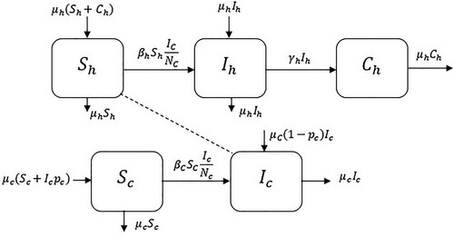
Figure 2. The plot shows fluctuation of ${\mathcal{R}}_0$ by considering changes in the values of ${\beta }_c$ and ${\mu }_c$.

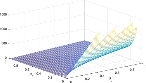
Figure 3. Fluctuation of ${\mathcal{R}}_0$ by considering changes in the values of ${\mu }_c$ and $p_c$.

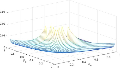
Figure 4. Fluctuation of ${\mathcal{R}}_0$ by considering changes in the values of ${\beta }_c$ and $p_c$.

Table 1. Sensitivity indices of ${\mathcal{R}}_0$.

Parameter	S. Index	Value
${\beta }_c$	$S_{{\beta }_c}$	1.000000
${\mu }_c$	$S_{{\mu }_c}$	-1.000000
$p_c$	$S_{p_c}$	-1.000000

4. Numeric imitations

In this section, we discuss diverse possible scenario to study the outcomes that some of the values of non-integer order $\mathcal{X}$ have on the stability of the toxoplasmosis disease in the population of human and cats. To check the dynamical consistency between the numerical and theoretical simulation of our proposed model, two different types of scenarios are calculated. The following Figure 1 shows the flow chart of the system. The two cases are disease free equilibrium and endemic equilibrium. These first one is stable if when ${\mathcal{R}}_0<1$ and the other one is stable if ${\mathcal{R}}_0>1$. Moreover, simulation is considered by taking into account the vertical transmission parameter $p_c$. This numerical simulation helps to study the effects of this parameter in the transmission dynamics toxoplasmosis disease of the population of the human and cat population. The graphical interpretation has been established via results of the system (23(23) $\begin{array}{r}\{\begin{array}{l}\frac{d^{\mathcal{X}}{X}_1}{d{\tau }^{\mathcal{X}}}={\mu }_h(1-X_1(\tau )-Y_1(\tau ))\\ -{\beta }_h{X}_1(\tau )(1-X_2(\tau )),\\ \frac{d^{\mathcal{X}}{Y}_1}{d{\tau }^{\mathcal{X}}}={\beta }_h{X}_1(\tau )(1-X_2(\tau ))-\gamma Y_1(\tau ),\\ \frac{d^{\mathcal{X}}{X}_2}{d{\tau }^{\mathcal{X}}}={\mu }_c{p}_c(1-X_2(\tau ))-{\beta }_c{X}_2(\tau )(1-X_2(\tau )),\end{array}\end{array}$(23) ). At this point, consider Adams Bashforth Moulton (PECE) technique using Matlab software.

Table 2. Values of the parameters of the model.

Stricture	DFE values	EE values	${\mathcal{R}}_0=1$	Unit	Source
${\mu }_h$	0.233	0.233	0.233	$Yea{r}^{-1}$	[35]
${\beta }_h$	0.0206	0.0206	0.0206	$Yea{r}^{-1}$	[35]
${\mu }_c$	0.066	0.066	0.066	$Yea{r}^{-1}$	[35]
γ	0.000232	0.000232	0.000232	$Yea{r}^{-1}$	[35]
$p_c$	0.01	0.0001	0.01	$Yea{r}^{-1}$	[35]
${\beta }_c$	0.000232	0.0008	0.00066	$Yea{r}^{-1}$	[35]

To study the effects of $\mathcal{X}$ on the dynamics of the system (23(23) $\begin{array}{r}\{\begin{array}{l}\frac{d^{\mathcal{X}}{X}_1}{d{\tau }^{\mathcal{X}}}={\mu }_h(1-X_1(\tau )-Y_1(\tau ))\\ -{\beta }_h{X}_1(\tau )(1-X_2(\tau )),\\ \frac{d^{\mathcal{X}}{Y}_1}{d{\tau }^{\mathcal{X}}}={\beta }_h{X}_1(\tau )(1-X_2(\tau ))-\gamma Y_1(\tau ),\\ \frac{d^{\mathcal{X}}{X}_2}{d{\tau }^{\mathcal{X}}}={\mu }_c{p}_c(1-X_2(\tau ))-{\beta }_c{X}_2(\tau )(1-X_2(\tau )),\end{array}\end{array}$(23) ), several numerical simulations have been performed by changing the values of the parameters. It is assumed a value for the parameter ${\beta }_c$ such that ${\mathcal{R}}_0<1$. It is shown in Figure 5 which is also expected from the theoretical consequences, the proposed system reaches to the TFE point. It is assumed a value for the parameter ${\beta }_c$ such that ${\mathcal{R}}_0>1$. Also, one can see that Figure 9 and as expected from the theoretical results, the system approaches to the endemic equilibrium point. 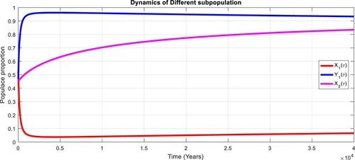Additionally, when ${\mathcal{R}}_0=1$, it can be observed in Figure 13 and simulations verify the theoretical outcomes. Figures 5–8 display that susceptible humans and susceptible cats have lower values and infected humans have higher values from the true equilibrium points. Figures 9–12 show that susceptible humans and susceptible cats have higher values and infected humans have lower values from the true equilibrium points as fractional order $\mathcal{X}$ goes down. Figure 5 shows that when the fractional index $\mathcal{X}=1$, the population of susceptible human and susceptible cat approaches to unity whereas the infected human approaches to zero, which verifies the theoretical results. Figures 6–8 show that susceptible human goes down to 0.73, 0.59, 0.21 whereas the infected human population increases to 0.27, 0.59 and 0.79. However, the populations of susceptible cat have minor decrease. Figure 9 shows that when the fractional index $\mathcal{X}=1$, the population of susceptible human and susceptible cat approaches to 0.02 whereas the infected human approaches to 0.98, which verifies the theoretical results. Figure 10–12 shows that susceptible human and cat remain same as for $\mathcal{X}=1$ whereas the infected human population is 0.98. Figure 13 shows that when the fractional index $\mathcal{X}=1$, the population of susceptible human and susceptible cat varies and infected human approaches whereas the infected human approaches to 0.98, which verifies the theoretical results. Figures 13–16 show that susceptible humans and susceptible cats have lower values and infected humans have higher values from the true equilibrium points as fractional order $\mathcal{X}$ goes down.

Figure 5. Dynamics of the diverse subpopulation at DFE point for $\mathcal{X}=1$, with ${\mathcal{R}}_0<1$.

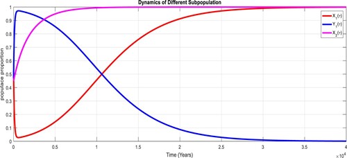
Figure 6. Dynamics of the diverse subpopulation at DFE point for $\mathcal{X}=0.95$, with ${\mathcal{R}}_0<1$.

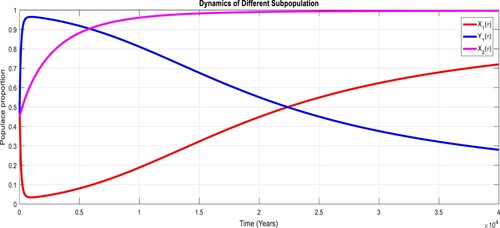
Figure 7. Dynamics of the diverse subpopulation at DFE point for $\mathcal{X}=0.90$, with ${\mathcal{R}}_0<1$.

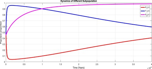
Figure 8. Dynamics of the diverse subpopulation at DFE point for $\mathcal{X}=0.85$, with ${\mathcal{R}}_0<1$.

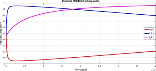
Figure 9. Dynamics of the diverse subpopulation at EE point for $\mathcal{X}=1$, with ${\mathcal{R}}_0>1$.

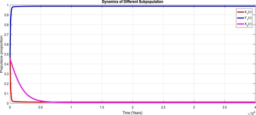
Figure 10. Dynamics of the diverse subpopulation at EE point for $\mathcal{X}=0.95$, with ${\mathcal{R}}_0>1$.

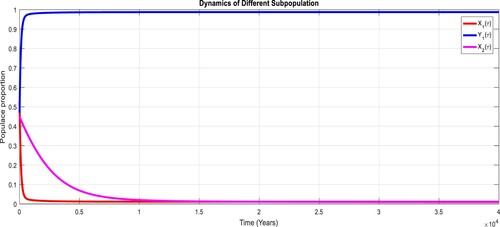
Figure 11. Dynamics of the diverse subpopulation at EE point for $\mathcal{X}=0.90$, with ${\mathcal{R}}_0>1$.

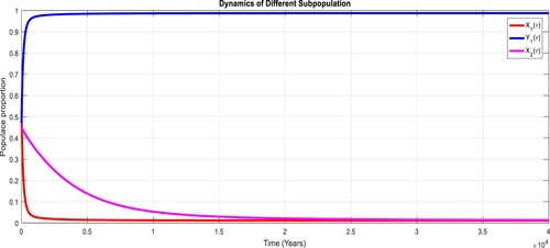
Figure 12. Dynamics of the diverse subpopulation at EE point for $\mathcal{X}=0.85$, with ${\mathcal{R}}_0>1$.

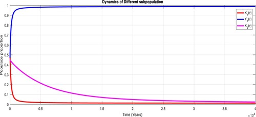
Figure 13. Dynamics of the diverse subpopulation point for $\mathcal{X}=1.00$, with ${\mathcal{R}}_0=1$.

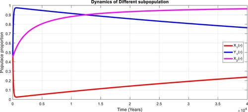
Figure 14. Dynamics of the diverse subpopulation point for $\mathcal{X}=0.95$, with ${\mathcal{R}}_0=1$.

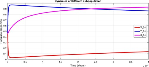
Figure 15. Dynamics of the diverse subpopulation point for $\mathcal{X}=0.90$, with ${\mathcal{R}}_0=1$.

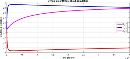
Figure 16. Dynamics of the diverse subpopulation point for $\mathcal{X}=0.85$, with ${\mathcal{R}}_0=1$.

Adams Bashforth Moulton algorithm

Here, we consider [51,52] to study the system (23(23) $\begin{array}{r}\{\begin{array}{l}\frac{d^{\mathcal{X}}{X}_1}{d{\tau }^{\mathcal{X}}}={\mu }_h(1-X_1(\tau )-Y_1(\tau ))\\ -{\beta }_h{X}_1(\tau )(1-X_2(\tau )),\\ \frac{d^{\mathcal{X}}{Y}_1}{d{\tau }^{\mathcal{X}}}={\beta }_h{X}_1(\tau )(1-X_2(\tau ))-\gamma Y_1(\tau ),\\ \frac{d^{\mathcal{X}}{X}_2}{d{\tau }^{\mathcal{X}}}={\mu }_c{p}_c(1-X_2(\tau ))-{\beta }_c{X}_2(\tau )(1-X_2(\tau )),\end{array}\end{array}$(23) ) for numerical simulation for different values of the order of the non-integer derivative, $\mathcal{X}\in (0,1]$. $\begin{array}{rl}{X}_1^{\mathrm{\aleph }+1}& =X_1(0)+\frac{h^{\mathcal{X}}}{\Gamma (\mathcal{X}+2)}\\ & \{{\mu }_h(1-(X_1{)}_{\mathrm{\aleph }+1}^p-(Y_1{)}_{\mathrm{\aleph }+1}^p)\\ & -{\beta }_h(X_1{)}_{\mathrm{\aleph }+1}^p(1-(X_1{)}_{\mathrm{\aleph }+1}^p)\}+\\ & \frac{h^{\mathcal{X}}}{\Gamma (\mathcal{X}+2)}\sum _{d=0}^{\mathrm{\aleph }}{a}_{j,\mathrm{\aleph }+1}\{{\mu }_h(1-(Y_1{)}_d)(1-(X_1{)}_d)\\ & -{\beta }_h(-(X_1{)}_d+1)(X_1{)}_d\},\end{array}$ $\begin{array}{rl}{Y}_1^{\mathrm{\aleph }+1}& =Y_1(0)+\frac{h^{\mathcal{X}}}{\Gamma (\mathcal{X}+2)}\\ & \{{\beta }_h(X_1{)}_{\mathrm{\aleph }+1}^p(1-(X_1{)}_{\mathrm{\aleph }+1}^p+\gamma (Y_1{)}_{\mathrm{\aleph }+1}^p)\}+\\ & \frac{h^{\mathcal{X}}}{\Gamma (\mathcal{X}+2)}\sum _{d=0}^{\mathrm{\aleph }}{a}_{j,\mathrm{\aleph }+1}\{{\beta }_h(X_1{)}_d(1-(X_1{)}_d)\\ & -\gamma (Y_1{)}_d\},\end{array}$ $\begin{array}{rl}{X}_2^{\mathrm{\aleph }+1}& =X_2(0)+\frac{h^{\mathcal{X}}}{\Gamma (\mathcal{X}+2)}\\ & \{{\mu }_c{p}_c(1-(X_2{)}_{\mathrm{\aleph }+1}^p)\\ & -{\beta }_c(X_2{)}_{\mathrm{\aleph }+1}^p(1-(X_2{)}_{\mathrm{\aleph }+1}^p)\}\\ & +\frac{h^{\mathcal{X}}}{\Gamma (\mathcal{X}+2)}\sum _{d=0}^{\mathrm{\aleph }}{a}_{j,\mathrm{\aleph }+1}\\ & \{{\mu }_c{p}_c(1-(X_2{)}_d)(1-(X_1{)}_d)\\ & -{\beta }_c(X_2{)}_d(1-(X_1{)}_d)\},\end{array}$ where $\begin{array}{rl}(X_1{)}_{\mathrm{\aleph }+1}^p& =X_1(0)+\frac{1}{\Gamma (\mathcal{X})}\sum _{d=0}^{\mathrm{\aleph }}{b}_{d,\mathrm{\aleph }+1}\\ & \{{\mu }_h(1-(X_1{)}_d-(Y_1{)}_d)\\ & -{\beta }_h(-(X_2{)}_d+1)(X_1{)}_d\},\\ (Y_1{)}_{\mathrm{\aleph }+1}^p& =Y_1(0)+\frac{1}{\Gamma (\mathcal{X})}\sum _{d=0}^{\mathrm{\aleph }}{b}_{d,\mathrm{\aleph }+1}\\ & \{{\beta }_h(-(X_2{)}_d+1))(X_1{)}_d-\gamma (Y_1{)}_d\},\\ (X_2{)}_{\mathrm{\aleph }+1}^p& =X_2(0)+\frac{1}{\Gamma (\mathcal{X})}\sum _{d=0}^{\mathrm{\aleph }}{b}_{d,\mathrm{\aleph }+1}\\ & \{{\mu }_c{p}_c(1-(X_2{)}_d)\\ & -{\beta }_c(X_2{)}_d(1-(X_2{)}_d)\},\end{array}$ with $\begin{array}{rl}& a_{d,\mathrm{\aleph }+1}\\ & \{\begin{array}{ll}{\mathrm{\aleph }}^{\mathcal{X}+1}-(\mathrm{\aleph }-\mathcal{X})(\mathcal{X}+1{)}^{\mathcal{X}},& d=0,\\ (-d+2+\mathrm{\aleph }{)}^{\mathcal{X}+1}+(-d+\mathrm{\aleph }{)}^{\mathcal{X}+1}\\ -2(-d+1+\mathrm{\aleph }{)}^{\mathcal{X}+1},& \mathrm{\aleph }\ge d\ge 1,\\ 1,& d=\mathrm{\aleph }+1,\end{array}\end{array}$ and $\begin{array}{rl}{b}_{d,\mathrm{\aleph }+1}& =\frac{h^{\mathcal{X}}}{\mathcal{X}}((-d+1+\mathrm{\aleph }{)}^{\mathcal{X}}-(-d+\mathrm{\aleph }{)}^{\mathcal{X}})\\ & 0\le d\le \mathrm{\aleph }.\end{array}$

5. Discussion and conclusion

In this article, we offer a nonlinear model to investigate the dynamics of non-integer order toxoplasmosis ailment in human and cat populations. The effects of the disease of toxoplasmosis on the population of human by taking the population of the cats as a transmission vector are considered. The system under observed consists of the modelling of the interaction between the susceptible and infective individuals of the two variates. It is assumed that the horizontal transmission of the disease to humans happens only through the contact with infected cats and vertical transmission in both populations of cats and humans. Further, it was assumed that the populations of cats and human are constant. It is also notable that the reproduction number ${\mathcal{R}}_0$ has the direct relationship to the probability of effective infectious which occurs due to the contact among the cats and does not depend on direct or indirect effective infectious contacts among humans and cats. Local and global stability of TFE and TPE points are debated. Adequate settings for steadiness of TFE point ${\mathcal{F}}^{\ast }$ are set in terms of the threshold parameter ${\mathcal{R}}_0$ of the model, where it is asymptotically stable if ${\mathcal{R}}_0<1$. The ailment persistent equilibrium point ${\mathcal{F}}^{\ast }$ exists when ${\mathcal{R}}_0>1$ and adequate settings that promise the asymptotic stability of this point are given. Moreover, sensitivity enquiry of the parameters convoluted in threshold parameter ( ${\mathcal{R}}_0$ ) are debated. Furthermore, the significance of feline's vertical transmission to the dynamics of the contagion is investigated through numeric imitations. When simulating the model with the specified algorithm, we have perceived that the method is congregating to ailment free and ailment persistent equilibrium points but through diverse trails for different values of fractional index $\mathcal{X}$ which are much closed at equilibrium points. The values are very close to each other to true equilibrium points. The fundamental objective of scrutinizing, such technique for toxoplasmosis disease model, is to support the scholars and policymakers in focusing on, treatment and prevention and resources for maximum greatest adequacy. At $\mathcal{X}=1$, the system behaves like the ordinary system as considered in [31,32] with comparable outcomes. In future research work, the authors will study the Lie algebra method [35,36] which is unique in its own kind and powerful tool, to find out the solution of different epidemic models which has sufficient symmetries.

Disclosure statement

No potential conflict of interest was reported by the author(s).

References

- Reyes-Lizano L, Chinchilla-Carmona M, Guerrero-Bermúdez OM, et al.Trasmisión de toxoplasma gondii en costa rica: un concepto actualizado. Acta Méd Cost. 2001;43(1):36–38.
- Dubey J. Duration of immunity to shedding of toxoplasma gondii oocysts by cats. J Parasitol. 1995;81(3):410–415.
- Sibley LD, Boothroyd JC. Virulent strains of Toxoplasma gondii comprise a single clonal lineage. Nature. 1992;359(6390):82–85.
- Kean B. Clinical parasitology. Am J Trop Med Hyg. 1984;33(3):515–516.
- Markell VMDJ. Parasitologíamédica, Mc Graw-Hill.
- Boothroyd JC, Grigg ME. Population biology of Toxoplasma gondii and its relevance to human infection: do different strains cause different disease? Curr Opin Microbiol. 2002;5(4):438–442.
- Zafar ZUA, Rehan K, Mushtaq M. Retracted article: fractional-order scheme for bovine babesiosis disease and tick populations. Adv Differ Equ. 2017;2017(1):1–19.
- Zafar ZUA, Mushtaq M, Rehan K. A non-integer order dengue internal transmission model. Adv Differ Equ. 2018;2018(1):1–23.
- Zafar ZUA, Rehan K, Mushtaq M, Rafiq M. Numerical treatment for nonlinear brusselator chemical model. J Differ Equ Appl. 2017;23(3):521–538.
- Zafar Z, Rehan K, Mushtaq M, Rafiq M. Numerical modeling for nonlinear biochemical reaction networks. Iran J Math Chem. 2017;8(4):413–423.
- Zafar ZUA, Ahmed M, Pervaiz A. Fourth order compact method for one dimensional inhomogeneous telegraph equation of o (h/sup 4/, k/sup 3/). Pakis J Eng Appl Sci. 2014;14 (1):96–101.
- Zafar ZUA, Rehan K, Mushtaq M. Hiv/aids epidemic fractional-order model. J Differ Equ Appl. 2017;23(7):1298–1315.
- Zafar ZUA, Mushtaq M, Rehan K, et al. Numerical simulation of fractional order dengue disease with incubation period of virus: fractional order dengue disease. Proc Pakis Acad Sci A Phys Comput Sci. 2017;54(3):277–296.
- Zafar ZUA, Rehan K, Mushtaq M, et al. Fractional numerical treatment for biochemical reaction networks: fractional biochemical reaction networks. Proc Pakis Acad Sci A Phys Comput Sci. 2017;54(3):297–304.
- Frenkel J, Ruiz A. Human toxoplasmosis and cat contact in Costa rica. Am J Trop Med Hyg. 1980;29(6):1167–1180.
- Rosso F, Les JT, Agudelo A, et al. Prevalence of infection with Toxoplasma gondii among pregnant women in Cali Colombia, South America. Am J Trop Med Hygiene. 2008;78(3):504–508.
- Yongzhen P, Xuehui J, Changguo L, et al. Dynamics of a model of toxoplasmosis disease in cat and human with varying size populations. Math Comput Simul. 2018;144:52–59.
- Arenas AJ, González-Parra G, Micó R-JV. Modeling toxoplasmosis spread in cat populations under vaccination. Theor Popul Biol. 2010;77(4):227–237.
- Lozano DFA. Modeling of parasitic diseases with vector of transmission: toxoplasmosis and babesiosis bovine [PhD Thesis]. Universitat Politècnica de València; 2011.
- Sunquist ME, Sunquist F. Kodkod Oncifelis guigna (Molina, 1782). In: Wild cats of the world. Chicago (IL): University of Chicago Press; 2002. p. 211–214.
- Deng H, Cummins R, Schares G, et al. Mathematical modelling of Toxoplasma gondii transmission: a systematic review. Food Waterborne Parasitol. 2020;22:e00102.
- Sullivan A, Agusto F, Bewick S, et al. A mathematical model for within-host Toxoplasma gondii invasion dynamics. Math Biosci Eng. 2012;9(3):647.
- Khan H, Khan A, Chen W, et al. Stability analysis and a numerical scheme for fractional Klein–Gordon equations. Math Methods Appl Sci. 2019;42(2):723–732.
- Shah K, Jarad F, Abdeljawad T. Stable numerical results to a class of time-space fractional partial differential equations via spectral method. J Adv Res. 2020;25:39–48.
- Gul H, Alrabaiah H, Ali S, et al. Computation of solution to fractional order partial reaction diffusion equations. J Adv Res. 2020;25:31–38.
- Ullah A, Ullah Z, Abdeljawad T, et al. A hybrid method for solving fuzzy volterra integral equations of separable type kernels. J King Saud Univ Sci. 2021;33(1):101246.
- Alrabaiah H, Ahmad I, Amin R, et al. A numerical method for fractional variable order pantograph differential equations based on haar wavelet. Eng Comput. 2021;1–14.
- Li T, Pintus N, Viglialoro G. Properties of solutions to porous medium problems with different sources and boundary conditions. Zeitsch Angew Math Phys. 2019;70:86.
- Murray JD. Mathematical biology I: an introduction. New York (NY): Springer; 2002.
- Brauer F, Castillo-Chavez C, Castillo-Chavez C. Mathematical models in population biology and epidemiology. Vol. 2. New York (NY): Springer; 2012.
- Ferreira JD, Echeverry LM, Rincon CAP. Stability and bifurcation in epidemic models describing the transmission of toxoplasmosis in human and cat populations. Math Methods Appl Sci. 2017;40(15):5575–5592.
- González-Parra GC, Arenas AJ, Aranda DF, et al. Dynamics of a model of toxoplasmosis disease in human and cat populations. Comput Math Appl. 2009;57(10):1692–1700.
- Shim E. A note on epidemic models with infective immigrants and vaccination. Math Biosci Eng. 2006;3(3):557.
- Miller KS, Ross B. An introduction to the fractional calculus and fractional differential equations. New York (NY): John Wiley & Sons; 1993.
- Shang Y. A lie algebra approach to susceptible-infected-susceptible epidemics. Electron J Differ Equ. 2012;2012(233):1–7.
- Shang Y. Analytical solution for an in-host viral infection model with time-inhomogeneous rates. Acta Phys Pol B. 2015;46(8):1567–1577.
- Viglialoro G, Woolley TE. Solvability of a Keller–Segel system with signal-dependent sensitivity and essentially sublinear production. Appl Anal. 2020;99(14):2507–2525.
- Podlubn I. Fractional differential equations. New York (NY): Academic; 1999.
- Wang Z, Yang D, Ma T, et al. Stability analysis for nonlinear fractional-order systems based on comparison principle. Nonlinear Dyn. 2014;75(1):387–402.
- Matignon D. Stability results for fractional differential equations with applications to control processing. In: Computational engineering in systems applications. Vol. 2, Citeseer; 1996. p. 963–968.
- Pinto CM, Carvalho AR. The role of synaptic transmission in a HIV model with memory. Appl Math Comput. 2017;292:76–95.
- Bohner M, Tunç O, Tunç C. Qualitative analysis of Caputo fractional integro-differential equations with constant delays. Comput Appl Math. 2021;40:214. DOI:https://doi.org/10.1007/s40314-021-01595-3
- Graef JR, Tunç C, Şevli H. Razumikhin qualitative analyses of Volterra integro-fractional delay differential equation with Caputo derivatives. Commun Nonlinear Sci Numer Simul. 2021. DOI:https://doi.org/10.1016/j.cnsns.2021.106037
- Khan H, Tunç C, Khan A. Stability results and existence theorems for nonlinear delay-fractional differential equations with Φp∗-operator. J Appl Anal Comput. 2020;10(2):584–597. DOI:https://doi.org/10.11948/20180322
- Tunç C, Golmankhaneh AK. On stability of a class of second alpha-order fractal differential equations. AIMS Math. 2020;5(3):2126–2142. DOI:https://doi.org/10.3934/math.2020141
- Tunç O, Atan Ö, Tunç C, et al. Qualitative analyses of integro-fractional differential equations with Caputo derivatives and retardations via the Lyapunov–Razumikhin method. Axioms. 2021;10(2):58. DOI:https://doi.org/10.3390/axioms10020058
- Huo J, Zhao H, Zhu L. The effect of vaccines on backward bifurcation in a fractional order HIV model. Nonlinear Anal Real World Appl. 2015;26:289–305.
- La Salle JP. The stability of dynamical systems. Philadelphia (PA): SIAM; 1976.
- Vargas-De-León C. Volterra-type Lyapunov functions for fractional-order epidemic systems. Commun Nonlinear Sci Numer Simul. 2015;24(1–3):75–85.
- Khan A, Hussain G, Inc M, et al. Existence, uniqueness, and stability of fractional hepatitis bepidemic model, Chaos: An interdisciplinary. J Nonlinear Sci. 2020;30(10):103104.
- Li C, Tao C. On the fractional Adams method. Comput Math Appl. 2009;58(8):1573–1588.
- Diethelm K, Ford NJ, Freed AD. A predictor–corrector approach for the numerical solution of fractional differential equations. Nonlinear Dyn. 2002;29(1):3–22.