Comparison of estimation methods for one-inflated positive Poisson distribution

Abstract

This paper aims to propose estimation methods for one-inflated positive Poisson (OIPP) distribution and compare their properties in terms of unbiasedness, consistency, efficiency and deficiency. All estimators considered in the study are asymptotically unbiased and consistent. The maximum likelihood estimator (MLE) for the OIPP distribution is asymptotically normal. When compared to the MLE, the ordinary least square estimator (OLSE) is the most efficient, followed by the method of moments estimator (MME) and the ratio of probability estimator (RPE). A novel one-inflation index was also proposed to assess the presence of excess ones in the dataset for the positive Poisson distribution to determine whether a one-inflated distribution is required for model fitting. A real dataset with a large number of ones, as identified by the proposed one-inflation index, was used for model fitting. It is found that the OLSE and MLE are the best estimators for an OIPP distribution.

KEYWORDS:

• Maximum likelihood
• one-inflation index
• ordinary least squares method
• ratio of probability
• zero-truncated Poisson

MSC2020:

• 60E05
• 62F10
• 62P25

1. Introduction

In discrete count data distribution, one method of modelling positive data is to truncate the distribution at zero, resulting in a zero-truncated distribution. Positive count data modelling can be traced back to the mid-twentieth century, when the first zero-truncated distribution, known as the zero-truncated Poisson distribution [1], was proposed. The probability mass function of the zero-truncated Poisson distribution is given as. $Pr\left(X=x|\lambda \right)=\frac{{\lambda }^x}{x!\left[\exp \left(\lambda \right)-1\right]};x=1,2,3,\dots ,$where $\lambda >0$ and the maximum likelihood estimator (MLE) of $\lambda$ can be obtained numerically by solving (1) $\overline{x}=\frac{{\hat{\lambda }}_1}{1-\exp \left(-{\hat{\lambda }}_1\right)}.$(1) Subsequently, other estimators for a zero-truncated Poisson distribution were developed and analysed [2–5]. An asymptotically unbiased estimator of $\lambda$ was proposed [2] as follows: (2) ${\hat{\lambda }}_2=\left(\sum _{x=0}^{r}x{n}_x\right)/\left(\sum _{x=0}^{r-1}{n}_x\right),$(2) where $n_x$ is the frequency of $x$-valued data and $r$ is the maximum number taken by $x$. Similarly, an efficient estimator of $\lambda$ was proposed [3] as follows: (3) ${\hat{\lambda }}_3=\frac{1}{n}\sum _{x=2}^{\mathrm{\infty }}x{n}_x,$(3)

Both (1) and (3) were used to estimate the mortality rate of the number of gall-cells per flower-head [4], and it was discovered that both estimators provide similar estimates for mortality rate estimation. In addition to the estimators in (1–3), a minimum variance unbiased estimator of $\lambda$ was proposed [5] as follows: (4) ${\hat{\lambda }}_4=\left\{\begin{array}{ll}\frac{t}{n}C\left(n,t\right);& 1\le n\le t,1\le t\\ & \le 50\text{ or }n=t\\ & \ge 51\text{ or }n=1,\\ & t\ge 51\\ \frac{t}{n}\left[1-{\left(\frac{n-1}{n}\right)}^{t-1}\right];& 2\le n\le 15,t\\ & \ge 51\text{ or }n\ge 16,\\ & t\gg n\\ {\hat{\lambda }}_1\text{ or }{\hat{\lambda }}_3;& \text{otherwise,}\end{array}\right.$(4) where $t=n\overline{x}$, $C\left(n,t\right)=1-S_{t-1}^{n-1}/S_t^n$ and $S_t^n$ is the Stirling number of the second kind. The function used for this estimator is dependent on the subdomain as shown in (4).

The negative binomial distribution was modified to the zero-truncated negative binomial distribution as an alternative to the zero-truncated Poisson distribution. As a result, the moment estimator for the zero-truncated negative binomial distribution was proposed [6] and further modified, resulting in a simpler but more efficient estimator [7]. A zero-truncated distribution based on the Poisson–Lindley distribution likelihood was also proposed, leading to the development of estimation methods based on the method of moments and maximum likelihood [8].

Inflated models based on the zero-truncated distribution have been studied to incorporate a large number of ones in the dataset. The proposed distributions include the one-inflated positive Poisson [9], one-inflated zero-truncated negative binomial [10], one-inflated positive Poisson mixture [11] and one-inflated positive Poisson–Lindley [12] models, which are all commonly used to estimate the population size of individuals in capture–recapture experiments. The inflation parameter in the one-inflated model is critical for reflecting the desire and ability of a captured subject to avoid recapture [9]. In line with [9], the goal of our study is to propose multiple estimation methods for an OIPP distribution and to identify the best estimators by considering various estimator properties. An inflation index that can assess the presence of excess ones in the dataset was also developed and analysed.

This paper is structured as follows: Section 2 provides a brief overview of the OIPP distribution and its statistical properties. Section 3 proposes estimation methods for an OIPP distribution. Section 4 discusses two simulation studies that were conducted to investigate the performance of the proposed estimation methods in terms of unbiasedness, consistency, efficiency and deficiency. Section 5 proposes a novel one-inflation index to assess the presence of excess ones in a dataset for the positive Poisson distribution to determine whether a one-inflated distribution is required for model fitting. The performance of the proposed index is also addressed in the same section. In Section 6, a dataset is fitted to the OIPP distribution using the proposed estimation methods and model fittings. Section 7 concludes the study.

2. One-inflated positive Poisson (OIPP) distribution and its statistical properties

Let $Y\sim OIPP\left(\omega ,\lambda \right)$, then the probability mass function of Y is given in (5), where $\lambda >0$ refers to the rate parameter and $\omega$ refers to the one-modification parameter for the oIPP distribution. (5) $Pr\left(Y=y|\omega ,\lambda \right)=\left\{\begin{array}{c}\omega +\left(1-\omega \right)\frac{\lambda }{\exp \left(\lambda \right)-1};y=1\\ \left(1-\omega \right)\frac{{\lambda }^y}{y!\left[\exp \left(\lambda \right)-1\right]};y\ge 2\end{array}\right.$(5) If $\omega >0$, then the distribution is known as an OIPP distribution [9]. If $\omega =0$, the OIPP distribution is reduced to a zero-truncated Poisson distribution [1]. It is possible for $\omega$ to be negative, such as $\omega \in \left(-\lambda /\left[\exp \left(\lambda \right)-1-\lambda \right],0\right)$, in which case the distribution is known as a one-deflated positive Poisson distribution. In this study, we restrict $\omega >0$ to ensure the one-inflation property. The formulae for the first two moments about the origin, the dispersion index and the moment generating function are given respectively as (6) $\begin{array}{rl}\mu & =\omega +\left(1-\omega \right)\frac{\lambda \exp \left(\lambda \right)}{\exp \left(\lambda \right)-1},\\ {\mu }_2& =\omega +\left(1-\omega \right)\frac{\lambda \exp \left(\lambda \right)\left[\lambda +1\right]}{\exp \left(\lambda \right)-1}=\mu +\left(\mu -\omega \right)\lambda ,\\ d& ={\sigma }^2/\mu =1+\lambda -\mu -\omega \lambda /\mu ,\\ M_Y\left(t\right)& =\omega \exp \left(t\right)+\left(1-\omega \right)\frac{\left\{\exp \left[\lambda \exp \left(t\right)\right]-1\right\}}{\exp \left(\lambda \right)-1}.\end{array}$(6)

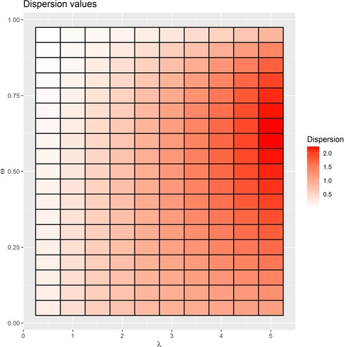
Figure 1 illustrates the dispersion index of various pairs of parameters $\lambda$ and $\omega$. The heatmap in Figure 1 shows that the OIPP distribution can be either underdispersed or overdispersed.

Figure 1. Heatmap of dispersion index for various pairs of parameters $\lambda$ and $\omega$.

For $y\ge 2$, the OIPP distribution is unimodal, which can be deduced based on the decreasing function from the following ratio: $\frac{Pr\left(Y=y+1|\omega ,\lambda \right)}{Pr\left(Y=y|\omega ,\lambda \right)}=\frac{\left(1-\omega \right)\frac{{\lambda }^{y+1}}{\left(y+1\right)!\left[\exp \left(\lambda \right)-1\right]}}{\left(1-\omega \right)\frac{{\lambda }^y}{y!\left[\exp \left(\lambda \right)-1\right]}}=\frac{\lambda }{y+1}.$

3. Estimation of parameters for OIPP distribution

Several estimation methods for an OIPP distribution were developed based on the method of moments, maximum likelihood, one-proportion, ratio of probability and ordinary least squares. Fitting a model to a dataset based on its method of moments, maximum likelihood and/or ordinary least squares estimators is a common practice in statistical modelling. On the other hand, the one-proportion and ratio of probability estimators are rarely used.

3.1. Method of moments estimator (MME)

The method of moments estimator (MME) is obtained by equating sample moments with theoretical moments. By equating the first two sample moments with the first two equations in (6), the MMEs of $\lambda$ and $\omega$ are obtained by solving. $\begin{array}{rl}& \left(1-m_1\right){\tilde{\lambda }}^2\exp \left(\tilde{\lambda }\right)+\left(m_2-m_1\right)\tilde{\lambda }\exp \left(\tilde{\lambda }\right)\\ & +\left(m_1-m_2\right)\left[\exp \left(\tilde{\lambda }\right)-1\right]=0\end{array}$and $\tilde{\omega }=\frac{\left(m_1-\tilde{\lambda }\right)\exp \left(\tilde{\lambda }\right)-m_1}{\exp \left(\tilde{\lambda }\right)-1-\tilde{\lambda }\exp \left(\tilde{\lambda }\right)},$where $m_k=\sum _{i=1}^n{y_i}^k/n$ for $n$ data, and $\tilde{\omega }$ and $\tilde{\lambda }$ are the respective MMEs of $\omega$ and $\lambda$.

3.2. Maximum likelihood estimation (MLE)

The log-likelihood function $l$ for a random variable Y that follows the OIPP distribution is given as. $\begin{array}{rl}& l\propto n_1\ln \left[\omega +\left(1-\omega \right)\frac{\lambda }{\exp \left(\lambda \right)-1}\right]\\ & +\left(n-n_1\right)\left\{\ln \left(1-\omega \right)-\ln \left[\exp \left(\lambda \right)-1\right]\right\}\\ & +\sum _{y=2}^{\mathrm{\infty }}{n}_y\ln \left(y\right),\end{array}$where $n_y$ refers to the number of $y$-valued observations and $n=\sum _{y=1}^{\mathrm{\infty }}{n}_y$. By differentiating $l$ with respect to $\omega$ and $\lambda$ and setting it to zero, the respective MLEs of $\omega$ and $\lambda$ can be obtained by solving $\hat{\omega }=\frac{n_1\left[\exp \left(\hat{\lambda }\right)-1\right]-n\hat{\lambda }}{n\left[\exp \left(\hat{\lambda }\right)-1-\hat{\lambda }\right]}$and $\left(\hat{\lambda }-A\right)\exp \left(\hat{\lambda }\right)+\left(A-1\right)\hat{\lambda }+A=0,$where $A=\left(n{m}_1-n_1\right)/\left(n-n_1\right)$ and $\hat{\omega }$ and $\hat{\lambda }$ are the respective MLEs of $\omega$ and $\lambda$.

A one-proportion estimator (OPE) is the extension to the estimator for the generalized negative binomial distribution. The OPE for the generalized negative binomial distribution can be obtained by comparing the first two sample moments and the sample proportion of zeros to the population proportion [13]. Similarly, the zero-inflated Poisson distribution parameter estimator is obtained by equating the empirical probability with the theoretical probability of zero-valued observations [14]. For the OIPP distribution, the OPE of $\omega$ is obtained by equating the theoretical proportion of ones to the sample proportion of one, while the OPE of $\lambda$ is obtained by equating the population mean to the sample mean. Surprisingly, the OPEs of $\omega$ and $\lambda$ are identical to their respective MLEs.

Theorem 1:

The MLE $\hat{\lambda }$ of $\lambda$ is consistent and asymptotically normal, such that. $\sqrt{n}\left(\hat{\lambda }-\lambda \right)\stackrel{d}{⟶}N\left(0,I^{-1}\left(\lambda \right)\right),$where $\begin{array}{rl}I\left(\lambda \right)& =\left[\omega +\left(1-\omega \right)\frac{\lambda }{u}\right]\\ & \times \frac{\begin{array}{c}\left[\right(1-\omega \left)uv\right(\lambda e^{\lambda })+e^{\lambda }(u-\lambda e^{\lambda })\\ \left(\omega u-v+1\right)+\omega u+1]\end{array}}{u^2{v}^2}\\ & +\frac{1-\omega }{\lambda }-\frac{e^{\lambda }\left(u-\lambda \right)\left(1-\omega \right)}{u^3}\end{array}$is the Fisher information of $\lambda$ with $u=\exp \left(\lambda \right)-1$ and $v=\omega \left(u-\lambda \right)+\lambda$.

Proof:

The regularity conditions under which the MLE $\hat{\lambda }$ is consistent and asymptotically normal is satisfied by the OIPP distribution (see [15, Chapter 6]), therefore $\begin{array}{rl}I\left(\lambda \right)& =-E\left(\frac{{\mathrm{\partial }}^2\ln f\left(y\right)}{\mathrm{\partial }{\lambda }^2}\right)\\ & =-E\left[\frac{{\mathrm{\partial }}^2}{\mathrm{\partial }{\lambda }^2}\left\{I_{\left(y=1\right)}\ln \left(\omega +\left(1-\omega \right)\frac{\lambda }{\exp \left(\lambda \right)-1}\right)\right.\right.\\ & +I_{\left(y>1\right)}(\ln (1-\omega )+y\ln \lambda \\ & -\left.\left.\ln y!-\ln \left(\exp \left(\lambda \right)-1\right))\phantom{\left(\omega +\left(1-\omega \right)\frac{\lambda }{\exp \left(\lambda \right)-1}\right)}\right\}\right]\\ & =-E\left[I_{\left(y=1\right)}P+I_{\left(y>1\right)}Q\right]=-\left[Pf\left(1\right)+\sum _{y=2}^{\mathrm{\infty }}Qf\left(y\right)\right],\end{array}$where $f\left(y\right)=Pr\left(Y=y\right)$, and $P$ and $Q$ are respectively given as $P=\frac{\begin{array}{c}\left(1-\omega \right)uv\left[-\lambda \exp \left(\lambda \right)\right]\\ -\exp \left(\lambda \right)\left[u-\lambda \exp \left(\lambda \right)\right]\left(\omega u-v+1\right)-\omega u-1\end{array}}{u^2{v}^2}$and $Q=-\frac{y}{{\lambda }^2}+\frac{\exp \left(\lambda \right)}{u^2}.$Solving the summation in $I\left(y\right)$ yields $\begin{array}{rl}I\left(\lambda \right)& =\left[\omega +\left(1-\omega \right)\frac{\lambda }{u}\right]\\ & \times \frac{\begin{array}{c}\left[\right(1-\omega \left)uv\right(\lambda e^{\lambda })+e^{\lambda }(u-\lambda e^{\lambda })\\ \left(\omega u-v+1\right)+\omega u+1]\end{array}}{u^2{v}^2}\\ & +\frac{1-\omega }{\lambda }-\frac{e^{\lambda }\left(u-\lambda \right)\left(1-\omega \right)}{u^3}.\end{array}$From Theorem 1, the asymptotic $100\left(1-\alpha \right)\mathrm{\%}$ confidence interval of $\lambda$ is given as. $\hat{\lambda }\mp z_{\alpha /2}\frac{I^{-1/2}\left(\lambda \right)}{\sqrt{n}}.\text{■}$

Theorem 2:

The MLE $\hat{\omega }$ of $\omega$ is consistent and asymptotically normal, such that $\sqrt{n}\left(\hat{\omega }-\omega \right)\stackrel{d}{⟶}N\left(0,I^{-1}\left(\omega \right)\right),$where $I\left(\omega \right)=\frac{\lambda -u}{u}\left\{\frac{\left(u-\lambda \right)\left[\omega \left(u-\lambda \right)+\lambda \right]}{v^2}+\frac{1}{1-\omega }\right\}$is the Fisher information of $\omega$ with $u=\exp \left(\lambda \right)-1$ and $v=\omega \left(u-\lambda \right)+\lambda$.

Proof:

The regularity conditions under which the MLE $\hat{\omega }$ is consistent and asymptotically normal is satisfied by the OIPP distribution (see [, Chapter 6]), therefore $\begin{array}{rl}I\left(\omega \right)& =-E\left(\frac{{\mathrm{\partial }}^2\ln f\left(y\right)}{\mathrm{\partial }{\omega }^2}\right)\\ & =-E\left[\frac{{\mathrm{\partial }}^2}{\mathrm{\partial }{\omega }^2}\left\{I_{\left(y=1\right)}\ln \left(\omega +\left(1-\omega \right)\frac{\lambda }{\exp \left(\lambda \right)-1}\right)\right.\right.\\ & +I_{\left(y>1\right)}(\ln (1-\omega )+y\ln \lambda \\ & -\left.\left.\ln y!-\ln \left(\exp \left(\lambda \right)-1\right))\phantom{\left(\omega +\left(1-\omega \right)\frac{\lambda }{\exp \left(\lambda \right)-1}\right)}\right\}\right]\\ & =-E\left[I_{\left(y=1\right)}R+I_{\left(y>1\right)}\frac{1}{{\left(1-\omega \right)}^2}\right]\\ & =-\left\{Rf\left(1\right)+\frac{1}{{\left(1-\omega \right)}^2}\left[1-f\left(1\right)\right]\right\},\end{array}$where $f\left(y\right)=Pr\left(Y=y\right)$ and $R=(u-\lambda {)}^2/v^2$.

Substituting $R$ in the derivation above yields $I\left(\omega \right)=\frac{\lambda -u}{u}\left\{\frac{\left(u-\lambda \right)\left[\omega \left(u-\lambda \right)+\lambda \right]}{v^2}+\frac{1}{1-\omega }\right\}.$Theorem 2 implies that the asymptotic $100\left(1-\alpha \right)\mathrm{\%}$ confidence interval of $\omega$ is given as $\hat{\omega }\mp z_{\alpha /2}\frac{I^{-1/2}\left(\omega \right)}{\sqrt{n}}.\text{■}$

3.3. Ratio of probability estimator (RPE)

The ratio of probability estimator (RPE) is the extension to the estimator for the generalized negative binomial distribution that can be obtained either by equating the ratio of one-valued observations to two-valued observations or by equating the first two theoretical moments with the sample moments [13]. The same method has been employed to obtain the parameter estimators for the zero-inflated Poisson–Lindley distribution [16]. Our study is premised on [13,16], in which the respective estimators of $\lambda$ and $\omega$ were obtained by considering the ratio of probability for 3-valued observations to 2-valued observations and by equating the population mean with the sample mean. Parameter $\omega$ can be eliminated by considering the ratio of probability for 3-valued observations to 2-valued observations, allowing parameter $\lambda$ to be easily obtained as follows: $\frac{Pr\left(Y=3|\omega ,\lambda \right)}{Pr\left(Y=2|\omega ,\lambda \right)}=\frac{\left(1-\omega \right)\frac{{\lambda }^3}{3!\left[\exp \left(\lambda \right)-1\right]}}{\left(1-\omega \right)\frac{{\lambda }^2}{2!\left[\exp \left(\lambda \right)-1\right]}}=\frac{\lambda }{3}.$By further equating $\lambda /3$ to the empirical ratio of $n_3/n_2$, the resulting RPE of $\lambda$ is given as $\stackrel{⌣}{\lambda }=3n_3/n_2,$where $\breve{\lambda }$ is the RPE of $\lambda$ and $\breve{\lambda }$ can only be obtained when both $n_2$ and $n_3$ are greater than zero. Note that the formula of $\breve{\lambda }$ is very simple, hence can be solved manually.

The calculation of RPE of $\omega$ is similar to the calculation of MME of $\omega$. Notice that the RPE of $\lambda$ is a special case of the general form of the Zelterman estimator studied by Böhning [17] given as $\left(i+1\right)n_{i+1}/n_i$, where $i=2$. Since the OIPP distribution is an extended zero-truncated Poisson distribution, it is only appropriate to use the first approach given by Böhning [17]. This entails truncating the Poisson model at all counts except 2 and 3, resulting in the following log-likelihood function. $\ell =\ln L={\left[\frac{1}{1+\frac{\lambda }{3}}\right]}^{n_2}{\left[\frac{\frac{\lambda }{3}}{1+\frac{\lambda }{3}}\right]}^{n_3},$with maximum likelihood estimate $\breve{\lambda }=3n_3/n_2=\breve{\lambda }$ (refer to [17] for a detailed explanation). Based on the findings in [17], the variance of RPE of $\lambda$, which is a special case of Zelterman estimator, can be written as $Var\left(\stackrel{⌣}{\lambda }\right)={\lambda }^2\left(\frac{1}{n_2}+\frac{1}{n_3}\right).$

The variance can be further estimated by substituting $\lambda$ with $\breve{\lambda }$, resulting in $V\hat{a}r\left(\stackrel{⌣}{\lambda }\right)=9\left[\frac{n_3}{{n_2}^3}\left(n_2+n_3\right)\right].$Identical results can be obtained using the second approach given by Böhning [17], which considers the nonparametric multinomial approach. Based on the variance and the estimated variance formulae, it can be concluded that the RPE of $\lambda$ is consistent since as $n$ increases, so does $n_i$. Also, the one-inflation and unimodality properties indicate that $n_2>n_3$, resulting in zero $Var\left(\breve{\lambda }\right)$ and $V\hat{a}r\left(\breve{\lambda }\right)$.

3.4. Ordinary least squares estimator (OLSE)

The ordinary least squares estimator (OLSE) is an estimator that minimizes the function of the squared difference between theoretical and empirical cumulative functions. Suppose $y_{\left(1\right)}\le y_{\left(2\right)}\le \dots \le y_{\left(n\right)}$ is the order statistics of the data that follows the OIPP distribution. It is known that $E\left[F\left(Y_{\left(i\right)}\right)\right]=i/\left(n+1\right)$ for $i=1,2,\dots ,n$. However, for count data, the expected value of the order statistics is best expressed with respect to the data frequency, such that $E\left[F\left(Y_{n_j}\right)\right]=\left(\sum _j^y{n}_j\right)/\left(n+1\right)$. The OLSE of $\omega$ and $\lambda$ can be obtained by minimizing the following function: $\begin{array}{rl}{S}_y\left(\omega ,\lambda \right)& =\sum _{y=1}^{\mathrm{\infty }}{\left[F\left(y|\omega ,\lambda \right)-\sum _{j=1}^y\frac{n_j}{n+1}\right]}^2\\ & =\sum _{y=1}^{\mathrm{\infty }}\left\{\sum _{j=1}^y\left\{\left[\omega +\left(1-\omega \right)\frac{\lambda }{\exp \left(\lambda \right)-1}\right]I_{\left(j=1\right)}\right.\right.\\ & +{\left.\left.(1-\omega )\frac{{\lambda }^j}{j!\left[\exp \left(\lambda \right)-1\right]}{I}_{\left(j>1\right)}\right\}-\frac{n_j}{n+1}\right\}}^2,\end{array}$where $I_{(\cdot )}$ is an indicator function and $n_y$ is the frequency of $y$-valued data. The estimators ${\omega }^{\ast }$ and ${\lambda }^{\ast }$ that give the smallest $S_y\left({\omega }^{\ast },{\lambda }^{\ast }\right)$ are the OLSEs of $\omega$ and $\lambda$, respectively. The resulting estimators have invariance property since OLSE is a special case of the minimum-distance estimation [18].

4. Simulation study

Two simulation studies were conducted to evaluate the performance of the proposed estimators in terms of unbiasedness, consistency and efficiency. Both simulation studies used $\lambda >1$ to ensure that $n_2>0$ and $n_3>0$, so that the RPEs of $\omega$ and $\lambda$ can be obtained.

4.1. Unbiasedness and consistency properties of the estimators

The first simulation study was conducted to evaluate the unbiasedness and consistency of the proposed estimators. The setting for the first simulation study is as follows:

Simulation setting:

Step 1. Generate $n=100,200,\dots ,1000$ random data samples that follow a positive Poisson distribution with parameters $\omega$ and $\lambda$, where $\omega =0.1,0.3$ and $\lambda =1.2,2.0$.

Step 2. Change the value of $\omega n$ data to 1 at random to ensure the one-inflation property.

Step 3. Estimate the parameters using MME, MLE, RPE and OLSE.

Step 4. Repeat Steps 1–3 for a total of 2000 times, and calculate bias $Bias\left({\delta }^{\mathrm{\prime }}\right)$ and mean squared error $MSE\left({\delta }^{\mathrm{\prime }}\right)$ for parameter $\delta$ using the following respective formulae $Bias\left({\delta }^{\mathrm{\prime }}\right)=\sum _{j=1}^{2000}|\delta -\delta {}_j^{\mathrm{\prime }}|/2000$and $MSE\left({\delta }^{\mathrm{\prime }}\right)=\sum _{j=1}^{2000}{\left(\delta -\delta {}_j^{\mathrm{\prime }}\right)}^2/2000,$where ${\delta }^{\mathrm{\prime }}$ is the estimated $\delta$ and $\delta =\omega ,\lambda$. The absolute value of the deviation about the true parameter was considered when computing the bias to provide a smooth trend of bias as $n$ increases and avoid bias value fluctuations.

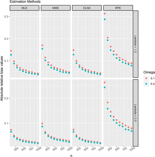
Figures 2 and 3 respectively illustrate the bias of the proposed estimators of $\lambda$ and $\omega$. Based on Figures 2 and 3, the following conclusions can be drawn:

1. The estimators are asymptotically unbiased. As $n$ increases, the bias of the estimators of both $\lambda$ and $\omega$ decrease and approach zero.

2. The biases of MMEs, MLEs and OLSEs are similar and significantly smaller than those of RPEs for the same sample size and parameters.

3. The estimators with the lowest to highest bias for any given sample size are MLE, OLSE, MME and RPE.

Figure 2. The absolute relative bias of the estimator of $\lambda$ when estimated using the MLE, MME, OLSE and RPE for $\lambda =1.2,2.0$ and $\omega =0.1,0.3$.

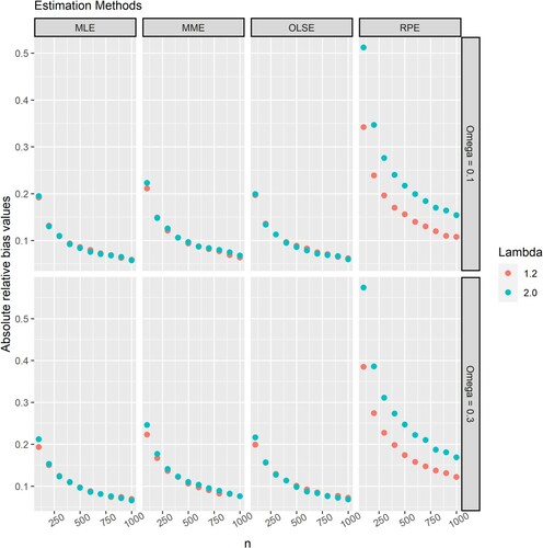
Figure 3. The absolute relative bias of the estimator of $\omega$ when estimated using the MLE, MME, OLSE and RPE for $\lambda =1.2,2.0$ and $\omega =0.1,0.3$.

Figures 4 and 5 respectively illustrate the mean squared error of the estimators of $\lambda$ and $\omega$ using the proposed estimation methods. Based on Figures 4 and 5, the following conclusions can be drawn:

1. The estimators are consistent for all parameters. As $n$ increases, the mean squared errors of the estimators decrease and approach zero.

2. The mean squared error of MMEs, MLEs and OLSEs are similar and significantly smaller than those of RPEs for the same sample size and parameters.

3. The estimators with the lowest to highest mean squared error for any given sample size are MLE, OLSE, MME and RPE.

Figure 4. The mean squared error of the estimator of $\lambda$ when estimated using the MLE, MME, OLSE and RPE for $\lambda =1.2,2.0$ and $\omega =0.1,0.3$.

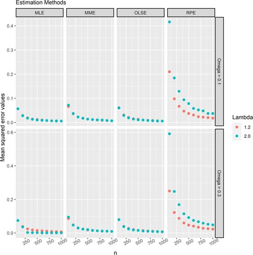
Figure 5. The mean squared error values of estimator $\omega$ when estimated using the MLE, MME, OLSE and RPE for $\lambda =1.2,2.0$ and $\omega =0.1,0.3$.

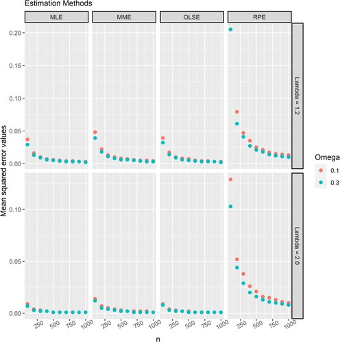
In short, the proposed estimators are asymptotically unbiased and consistent for all values of parameters. RPE has a significantly larger bias and mean squared error than other estimators, but it still may provide a good model fitting for very large samples $\left(\text{n}\gg 1000\right)$. The best to worst estimators in terms of unbiasedness and consistency are MLE, OLSE, MME and RPE.

4.2. Efficiency property of the estimators

The second simulation study was conducted to evaluate the efficiency of the proposed estimators compared to the efficiency of the MLE. The setting for the second simulation study is as follows:

Simulation setting:

Step 1. Generate $n=1000$ random data samples that follow the positive Poisson distribution with parameters $\omega$ and $\lambda$.

Step 2. Change the value of $\omega n$ data to 1 at random to ensure the one-inflation property.

Step 3. Estimate the parameters using MME, MLE, RPE and OLSE.

Step 4. Repeat Steps 1–3 for a total of 2000 times, and calculate the efficiency of all estimators compared to the efficiency of the MLE using $eff\left({\delta }^{\mathrm{\prime }},\hat{\delta }\right)=Var\left(\hat{\delta }\right)/Var\left({\delta }^{\mathrm{\prime }}\right),$where ${\delta }^{\mathrm{\prime }}$ is the MME, RPE and OLSE of $\delta$, and $\hat{\delta }$ is the MLE of $\delta$. Since the asymptotically unbiased property has been established and variance can be represented as the sum of mean squared error and squared bias, the efficiency of the estimators can be calculated using the following formula: $eff\left({\delta }^{\mathrm{\prime }},\hat{\delta }\right)=MSE\left(\hat{\delta }\right)/MSE\left({\delta }^{\mathrm{\prime }}\right).$

Figure 6 and Figure 7 respectively illustrates the efficiency of the proposed estimators of $\lambda$ and $\omega$ in percentage compared to the efficiency of the MLE. Based on Figure 6 and Figure 7, the following conclusions can be drawn:

1. The MME of $\lambda$ is approximately 70–80% as efficient as the MLE of $\lambda .$

2. The MME of $\omega$ is approximately 40–70% as efficient as the MLE of $\omega .$

3. The RPE of $\lambda$ is approximately 5–30% as efficient as the MLE of $\lambda .$

4. The RPE of $\omega$ is approximately 2–25% as efficient as the MLE of $\omega .$

5. The OLSEs of $\lambda$ and $\omega$ is approximately 90–99% as efficient as the MLE of $\lambda$ and $\omega$.

Figure 6. The efficiency of the estimators of $\lambda$ when estimated using the MME, RPE and OLSE with respect to the MLE.

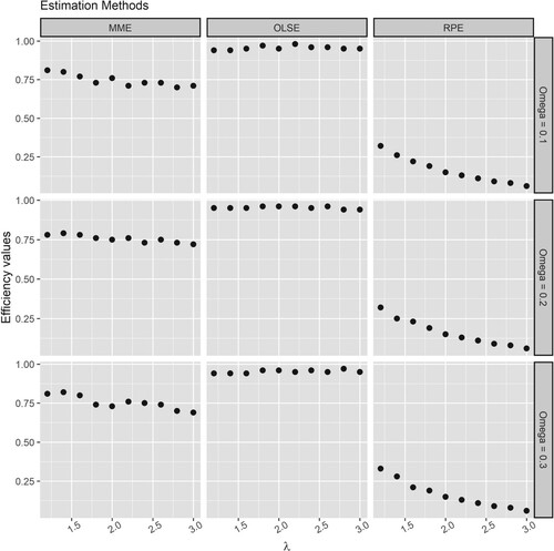
Figure 7. The efficiency of the estimators of $\omega$ when estimated using the MME, RPE and OLSE with respect to the MLE.

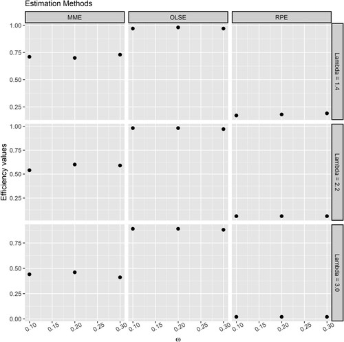
It can be concluded that the OLSE is almost as efficient as the MLE but more efficient than the MME and RPE. Also, the MME is significantly more efficient than the RPE.

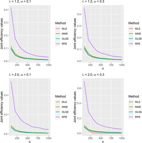
Another way to evaluate estimator performance is by calculating the joint efficiencies of the estimators for the two parameters using the deficiency criterion [19], which is defined as. $Def\left({\lambda }^{\mathrm{\prime }},{\omega }^{\mathrm{\prime }}\right)=MSE\left({\lambda }^{\mathrm{\prime }}\right)+MSE\left({\omega }^{\mathrm{\prime }}\right),$where ${\lambda }^{\mathrm{\prime }}$ and ${\omega }^{\mathrm{\prime }}$ are the estimators of $\lambda$ and $\omega$, respectively. Figure 8 shows that the joint efficiency decreases as the sample size grows for given $\lambda$ and $\omega$. The MLE, MME and OLSE have similar joint efficiencies, whereas RPE has a substantially larger joint efficiency, even when the sample size is as large as 1000. According to the deficiency criterion, the MLE is the most efficient estimator. The estimators with the best to worst efficiency are MLE, OLSE, MME and RPE. These findings corroborate the findings in Figure 6 and Figure 7.

Figure 8. The joint efficiency of the estimators of $\lambda$ and $\omega$ when estimated using the MLE, MME, OLSE and RPE for $\lambda =1.2,2.0$ and $\omega =0.1,0.3$.

5. One-inflation index under positive Poisson distribution

A novel index called the one-inflation index was developed to determine whether a one-inflated distribution is required to model a dataset. By definition, a $k$-inflation index is an index that assesses the presence of $k$-valued data with respect to a certain distribution. For instance, the zero-inflation index, denoted as $z{i}_p$, assesses the presence of excess zeros in a dataset for a Poisson distribution [20,21]. Another zero-inflation index, denoted as $z{i}_{nb}$, was introduced to assess the presence of excess zeros in the dataset for a negative binomial distribution [22]. The formulae of $z{i}_p$ and $z{i}_{nb}$ are respectively given as. $z{i}_p=1+\ln \left(p_0\right)/\mu$and $z{i}_{nb}=1+\frac{\left({\sigma }^2-\mu \right)\ln \left(p_0\right)}{{\mu }^2\ln \left({\sigma }^2/\mu \right)},$where $p_0$ is the proportion of zeros, $\mu$ is the mean and ${\sigma }^2$ is the variance. When the sample zero-inflation index is greater than zero, this indicates that there are excess zeros in the dataset. Following the works in [20–22], a new one-inflation index is proposed to assess the presence of excess ones in the dataset for a positive Poisson distribution. The one-inflation index is denoted as $o{i}_{pp}=1+\frac{\ln \left(p_1\right)}{\ln \left[\exp \left(d+\mu -1\right)-1\right]-\ln \left(d+\mu -1\right)},$where $p_1$ is the proportion of ones and $d$ is the dispersion index. If a random variable follows the positive Poisson distribution, then $o{i}_{PP}=0$, while $o{i}_{PP}>0$ indicates that the dataset contains a large number of ones for the positive Poisson distribution. The presence of excess ones in the sample data can be determined by computing the sample one-inflation index. As an example, a dataset of size 5000 that follows the OIPP distribution was simulated, and the one-inflation index $\hat{o}{i}_{PP}$ for a positive Poisson distribution are shown in Table 1.

Table 1. The sample proportion of one-valued data, sample mean, sample variance, sample dispersion index and sample one-inflation index for the one-inflated positive Poisson distribution for various pairs of parameters $\lambda$ and $\omega$, based on a dataset of size 5000.

$\lambda$	$\omega$	Sample proportion, ${\hat{p}}_1$	Sample mean,$\overline{y}$	Sample variance,$s^2$	Sample dispersion index, $\hat{d}$	Sample index, $\hat{o}{i}_{PP}$
0.5	0.0	0.768	1.276	0.296	0.232	0.006
	0.2	0.815	1.218	0.246	0.202	0.061
	0.4	0.866	1.163	0.198	0.171	0.158
	0.6	0.909	1.108	0.135	0.122	0.185
1.0	0.0	0.584	1.581	0.664	0.420	0.007
	0.2	0.664	1.464	0.574	0.392	0.108
	0.4	0.756	1.336	0.453	0.339	0.214
	0.6	0.837	1.234	0.359	0.291	0.352
1.5	0.0	0.432	1.936	1.135	0.586	0.019
	0.2	0.539	1.748	1.015	0.580	0.161
	0.4	0.658	1.553	0.852	0.549	0.304
	0.6	0.767	1.383	0.666	0.482	0.428
2.0	0.0	0.317	2.302	1.582	0.687	0.004
	0.2	0.439	2.081	1.637	0.786	0.234
	0.4	0.589	1.788	1.369	0.766	0.395
	0.6	0.726	1.512	1.027	0.679	0.511
2.5	0.0	0.223	2.743	2.173	0.792	0.014
	0.2	0.384	2.369	2.154	0.910	0.289
	0.4	0.529	2.062	2.054	0.996	0.469
	0.6	0.692	1.684	1.533	0.911	0.592

According to Table 1, the index correctly assesses the presence of excess ones in the sample data. When $\omega =0$, this implies that the index is very close to zero, which indicates that there is no excess of ones in the data for the OIPP distribution since this distribution reduces to a positive Poisson distribution. Trivially, a smaller $\lambda$ yields a higher proportion of ones in the positive Poisson distribution and a lower proportion of ones contributed by $\omega$ in the OIPP distribution. Therefore, the resulting index will be comparatively low (refer to Table 1 for $\lambda =0.5$ and all values of $\omega$). However, when $\lambda$ is large, the proportion of ones in the positive Poisson distribution will be small, while the proportion of ones contributed by $\omega$ in the OIPP distribution will be large. This results in a high index value (refer to Table 1 for $\lambda =2.5$ and positive $\omega$). It can be concluded that the one-inflation index is useful to assess the presence of excess ones in a dataset for a positive Poisson distribution.

This one-inflation index can be a viable alternative to the score test proposed by Godwin and Böhning [9], in which the null hypothesis of the test states that there is no inflation in the data. The score test [9] is given as. $S=\frac{{\left(\frac{n_{1}T}{\hat{\lambda }}-n\right)}^2\hat{\lambda }\left(T+1\right)}{nT\left(T-\hat{\lambda }\right)}$where $T=\exp \left(\hat{\lambda }\right)-1$ and $S\sim {{\chi }^2}_{\left(1\right)}$. The information about whether a dataset contains excess ones or not needs to be considered in statistical modelling. If the dataset contains excess ones, then one-inflated positive count data distributions should be considered.

6. Applications

A dataset on the frequency of a person being arrested for drunk driving [23] was used to demonstrate and analyse the performance of the proposed estimators in fitting real data. The sample one-inflation index of 0.1545 implies that the dataset contains a substantial number of ones in the data that cannot be explained by a positive Poisson distribution. The model fitting to the data using a positive Poisson distribution yields $\hat{\lambda }=0.1275$. The estimated value of $\lambda$ generates a score $s=30.6686$, hence rejecting the null hypothesis of no inflation. Therefore, the OIPP distribution is appropriate for model fitting for this dataset.

The chi-square goodness-of-fit test and the root mean squared error (RMSE) of the fitted data were used to evaluate the proposed estimators, in which $RMSE=\sqrt{\sum _{x=1}^h{\left(n_x-{\hat{n}}_x\right)}^2/h},$ where $h$ is the number of data groups and ${\hat{n}}_x$ is the estimated frequency for the respective $n_x$. In general, the best estimator provides adequate goodness of fit and has the lowest RMSE.vn

The results of the model fitting for the frequency of a person being arrested for drunk driving based on the proposed estimators are shown in Table 2. Based on the goodness-of-fit test and p-values, all estimators are found to be adequate except for RPE. The RMSE of the OLSE is found to be significantly smaller compared to other estimators. Therefore, the OLSE provide the best fit for describing the frequency of a person being arrested for drunk driving.

Table 2. The results of model fitting of the frequency of a person being arrested for drunk driving based on the MME, MLE, RPE and OLSE for the OIPP distribution.

		Estimators
$x$	$n_x$	MME	MLE	RPE	OLSE
1	8877	8880.44	8876.98	8868.79	8876.96
2	481	471.05	477.33	492.38	480.36
3	52	61.08	58.82	53.23	56.35
4	8	5.94	5.44	4.32	4.96
5+	1	0.49	0.44	0.28	0.37
Estimated parameters	$\lambda$	0.3890	0.3697	0.3243	0.3519
	$\omega$	0.6857	0.6683	0.6192	0.6526
	RMSE	6.29	3.66	6.52	2.41
	${\chi }^2$	2.5885	2.4745	4.5077	2.8637
	df	1	1	1	1
	p-value	0.1076	0.1157	0.0337	0.0906

* the best model is written in bold.

7. Conclusions

Several estimators for the OIPP distribution were proposed in this study, namely MME, MLE, RPE, OPE and OLSE, in which the MLE and OPE both yield identical results. Two comprehensive simulation studies were conducted to evaluate the unbiasedness, consistency and efficiency of the proposed estimators. According to the results, the proposed estimators are asymptotically unbiased and consistent. The best to worst estimators based on the bias, mean squared error, efficiency and deficiency values are MLE, OLSE, MME and RPE. A one-inflation index to assess the presence of excess ones in a dataset for a positive Poisson distribution was also proposed. Based on the chi-square goodness-of-fit test and RMSE, the OLSE provides the best fit to the dataset adopted in this study. Therefore, both MLE and OLSE are the best estimators for the OIPP distribution.

Acknowledgements

The authors gratefully acknowledge the financial support received in the form of research grants from the Ministry of Education, Malaysia [FRGS/1/2019/STG06/UKM/01/5]; and Universiti Kebangsaan Malaysia [GUP-2019-031].

Disclosure statement

No potential conflict of interest was reported by the author(s).

Additional information

Funding

This work was supported by Ministry of Education, Malaysia: [Grant Number FRGS/1/2019/STG06/UKM/01/5]; Universiti Kebangsaan Malaysia: [Grant Number GUP-2019-031].

References

- David FN, Johnson NL. The truncated Poisson. Biometrics. 1952;8:275–285.
- Moore PG. The estimation of the Poisson parameter from a truncated distribution. Biometrika. 1952;39:247–251.
- Plackett RL. The truncated Poisson distribution. Biometrics. 1953;9:485–488.
- Finney DJ, Varley GC. The truncated Poisson distribution. Biometrics. 1955;11:387–394.
- Tate RF, Goen RL. Minimum variance unbiased estimation for the truncated Poisson distribution. Ann Math Stat. 1958;29:755–765.
- Sampford MR. The truncated negative binomial distribution. Biometrika. 1955;42:58–69.
- Brass W. Simplified methods of fitting the truncated negative binomial distribution. Biometrika. 1958;45:59–68.
- Ghitany ME, Al-Mutairi DK, Nadarajah S. Zero-truncated Poisson-Lindley distribution and its application. Math Comput Simul. 2008;79:279–287.
- Godwin RT, Böhning D. Estimation of the population size by using the one-inflated positive Poisson model. J R Stat Soc: Ser C. 2017;66:425–448.
- Godwin RT. One-inflation and unobserved heterogeneity in population size estimation. Biometrical J. 2017;59:79–93.
- Godwin R. The one-inflated positive Poisson mixture model for use in population size estimation. Biometrical J. 2019;61:1541–1556.
- Tajuddin, R. R. M., Ismail, N., Kamarulzaman, I., 2021. Estimating population size of criminals: a new Horvitz-Thompson estimator under one-inflated positive Poisson-Lindley model. Crime & Delinquency. doi:10.1177%2F00111287211014158
- Famoye F. Parameter estimation for generalized negative binomial distribution. Commun Stat – Simu Comput. 1997;26:269–279.
- Wagh YS, Kamalja KK. Zero-inflated models and estimation in zero-inflated Poisson distribution. Commun Stat – Simu Comput. 2018;47:2248–2265.
- Hogg, R.V., McKean, J.W., Craig, A.T. Maximum likelihood estimation, in Introduction to mathematical statistics, 6th ed. Pearson Prentice Hall, New Jersey, pp. 313, 2005.
- Borah M, Nath AD. A study of the inflated Poisson Lindley distribution. J Indian Soc Agr Stat. 2001;54:317–323.
- Böhning D. A simple variance formula for population size estimators by conditioning. Stat Methodol. 2008;5:410–423.
- Drossos CA, Philippou AN. A note on minimum distance estimates. Ann I Stat Math. 1980;32:121–123.
- Akgül FG, Şenoğlu B, Arslan T. An alternative distribution to Weibull for modeling the wind speed data: Inverse Weibull distribution. Energ Convers Manage. 2016;114:234–240.
- Puig P. Characterizing additively closed discrete models by a property of their maximum likelihood estimators, with an application to generalized Hermite distributions. J Am Stat Assoc. 2003;98:687–692.
- Puig P, Valero J. Count data distributions. J Am Stat Assoc. 2006;101:332–340.
- Blasco-Moreno A, Pérez-Casany M, Puig P, et al. What does a zero mean? Understanding false, random and structural zeros in ecology. Methods Ecol Evol. 2019;10:949–959.
- Van der Heijden PGM, Cruyff M, Van Houwelingen HC. Estimating the size of a criminal population from police records using the truncated Poisson regression model. Statistica Neerlandica. 2003;57:289–304.