
 ?Mathematical formulae have been encoded as MathML and are displayed in this HTML version using MathJax in order to improve their display. Uncheck the box to turn MathJax off. This feature requires Javascript. Click on a formula to zoom.
Abstract
Entropy is a measure of random variable uncertainty that reflects the anticipated quantity of information. In this paper, estimation of Shannon entropy for Lomax distribution, viz unified hybrid censored data are considered. The processes of maximum likelihood and Bayesian estimation procedures are regarded. The Bayesian estimator under balanced squared error, balanced linear exponential, and balanced general entropy loss functions are derived. The purpose of a Monte Carlo simulation study is designed to compare the accuracy of different estimators in the context of specific measures. Real data analysis is employed to confirm the proposed estimators. In summary, we discovered that, according to the findings of the study, the mean squared errors values decrease as the sample size increases. In the majority of cases, Bayesian estimates under balanced linear exponential loss function are more appropriate in terms of simulation out comes than other specified loss functions.
1. Introduction
Due to a lack of funding and time constraints in the majority of life's trials, it is better to stop the test before all of the items fail. Censored samples are the observations that arise from that situation, and there are numerous censoring strategies. The most common types of censorship are type I (T-I) and type II (T-II). The test is completed at a predetermined censoring time in T-I censoring. The test is completed at a fixed number of failures in T-II censorship. The hybrid censoring scheme (HCS) is a combination of T-I and T-II censoring methods that can be characterized as below.
In a life-testing setting, assume there are n identical items with lifetimes are identically distributed and independent. Let be the ordered failure times of these objects. When a prefixed number of items,
, out of n, fail, or when a prefixed period
is reached, the test is ended. Epstein [Citation1] was the first to propose this hybrid censoring method, and there are two types: T-I HCS and T-II HCS.
The life-testing experiment in T-I HCS is completed at a random time . The disadvantage of T-I HCS is that very few failures occur until the predetermined period
. To address this flaw, Childs et al. [Citation2] suggested a recently HCS known as T-II HCS, which ensures fixed number of failures and has a termination time
. Although the T-II HCS ensures a specific amount of failures, detecting failures and completing the life test can take a lengthy time, which is a disadvantage. These techniques were modified by Chandrasekar et al. [Citation3], who introduced generalized T-I HCS (GT-I HCS) and generalized T-II HCS (GT-II HCS).
One fixes and time
in GT-I HCS, where
.
, if the
failure appears before the time T.
if the
failure occurs after the time T. In GT- II HCS,
and
are chosen so that
.
if the
failure occurs before time
;
if there is the
failure between
and
; otherwise,
. Even while these two new censored sampling systems outperform the previous ones, they nevertheless have flaws. Because there is just one the pre-assigned period T in GT-I HCS, we cannot ensure r failures. There is a chance that the GT-II HCS will not see a few failures until a pre-determined time
, and so it will have the same trouble as the T-I HCS. To overcome the shortcomings of both systems, Balakrishnan et al. [Citation4] proposed a scheme that combines GT-I HCS and GT-II HCS and is referred to the unified hybrid censoring scheme (UHCS).
Fix the integers and the time points
in this scheme.
, if the kth failure happened prior to time
.
if the kth failure happens between
and
, and
, if the kth failure happens after
. Using this scheme strategy, we can confirm that the test will be finished in time
with at least k failures, if not, exactly k failures. See [Citation5] for more details on how well the difficulties in the previous types were resolved in this manner. As a result, we have the six cases indicated in Figure under this UHCS:
Figure 1. Unified hybrid censoring scheme.
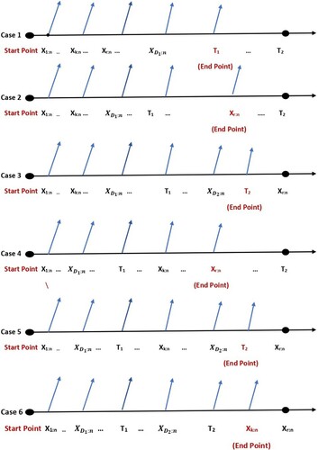
Case 1: , if this is the case, we will end at
,
Case 2: , if this is the case, we will end at
,
Case 3: , if this is the case, we will end at
,
Case 4: , if this is the case, we will end at
,
Case 5: , if this is the case, we will end at
,
Case 6: , if this is the case, we will end at
.
Entropy is a key concept in statistics and information theory, and it was first recommended in physics second law of thermodynamics. Shannon [Citation6] re-defined it and introduced the idea of entropy into information theory to quantify information uncertainty. Cover and Thomas [Citation7] built on Shannon's notion, defining differential entropy (or continuous entropy) of a continuous random variable X with probability density function as follows:
(1)
(1) Entropy measurement is a crucial concept in a variety of fields. More entropy indicates that there is less information in the sample.
Shannon entropy has many applications in many fields see [Citation8,Citation9] in physics and other fields can be found in [Citation10–13].
Entropy in hybrid censoring data studied by Morabbi and Razmkhah [Citation14]. In progressive censoring of T-II, Abo-Eleneen [Citation15] looked at the entropy and the best method. Cho et al. [Citation16] used doubly GT-II HCS to calculate the entropy of the Rayleigh distribution. Liu and Gui [Citation17] investigated entropy estimate for the Lomax distribution using maximum likelihood (ML) and Bayesian methods under generalized progressively hybrid censoring. Under multiple censored data, Hassan and Zaky [Citation18] found the ML estimator of Shannon entropy for the inverse Weibull distribution. The Shannon entropy of the inverse Weibull distribution under progressive first-failure censoring was investigated by Yu et al. [Citation19]. Bantan et al. [Citation20] investigated entropy estimation of inverse Lomax distribution viz multiple censored data.
The study of inference problems associated with entropy measures has recently gained prominence. As previously stated, the UHCS may be able to overcome the restrictions of the GT-I HCS and GT-II HCS. The Lomax distribution, on the other hand, it has sparked scholarly interest in the last decade due to its possible uses in a range of domains, including lifetime data prediction. We could not discover any study on the Shannon entropy measure estimation problem using UHCS in this regard. Consequently, the main purpose of this study is to use the UHCS to derive ML and Bayesian estimators from the Lomax distribution. Three losses are used to create a Bayesian estimator for Shannon entropy. The balanced-squared error loss (BSEL) function, balanced linear-exponential (BLINEX) loss function, and the balanced general entropy (BGE) loss function are used to create a Bayesian estimate for Shannon entropy. The Markov chain Monte Carlo (MCMC) strategy is employed to solve Bayesian entropy estimators with balanced loss functions. A numerical evaluation is used to assess the behaviour of the provided estimates via UHCS. Real data is analysed for more evidence, allowing the theoretical results to be confirmed.
This paper is planned as follows: The Shannon entropy for the Lomax distribution is calculated in Section 2. The ML Shannon entropy estimator is shown in Section 3. Section 4 covers the MCMC method for calculating Bayesian estimators and derives the Bayesian estimator of entropy under various loss functions. Simulation issue and application to real data are given in Sections 5 and 6, respectively. Section 7 brings the article to a close with some last thoughts.
2. Lomax distribution
Lomax (Lo) distribution is one of the important lifetime models. It has been useful in reliability and life testing problems (see, Hassan and Al-Ghamdi [Citation21]). Lo distribution was first introduced by Lomax [Citation22] and it is useful in a variety of domains, including actuarial science and economics. The Lo distribution was applied to income and wealth data see [Citation23,Citation24]. More details about applications of Lo distribution can found in [Citation25,Citation26].
A random variable is said to have Lo distribution with shape parameter α and scale parameter ϕ if its probability density function (pdf) is given by
(2)
(2) The cumulative distribution function (cdf) of X is given by
(3)
(3) Various studies about Lo distribution can be found in the literature by several authors. Some recurrence relations between the moments of record values from the Lo distribution were studied by Balakrishnan and Ahsanullah [Citation27]. On the basis of T-II censored data, Okasha [Citation28] studied E-Bayesian estimate for the Lo distribution. Singh et al. [Citation29] explored Bayesian estimation of Lo distribution under T-II HCS using Lindley's approximation. Statistical inference of Lo distribution using some information measures can be found in [Citation30–32].
Substituting (Equation2(2)
(2) ) into (Equation1
(1)
(1) ) will give the Shannon entropy of the Lo distribution
Hence,
(4)
(4) To compute H(x) in (Equation4
(4)
(4) ), we must calculate
and
and
Using integration rules we get
(5)
(5) To obtain
, let
then
, so
will be
then, using integration by parts we can find the value of the integral
then,
(6)
(6) As a result, the Shannon entropy of the Lo distribution looks like this:
(7)
(7) As a function of parameters α and ϕ, this is the needed formulation of Shannon entropy of the Lo distribution.
3. Maximum likelihood estimation
Under UHCS, the ML estimation of the Lo distribution is discussed in this section. Assume there are n identical items in a life-testing experiment. Let represent the ordered failure times of these items, with fixed integer
where
and time points
where
. Then the likelihood function of α and ϕ, for six cases of UHCS is given by
(8)
(8) where D is total number of failures up to time c in the experiment, and its value in the statements given by
(9)
(9) where
and
refer to the number of failures prior to
and
, respectively. Substituting (Equation2
(2)
(2) ) and (Equation3
(3)
(3) ) in (Equation8
(8)
(8) ) we obtain
this equation can be written in the following way:
(10)
(10) where
. Taking the logarithm of both sides we get
(11)
(11) where
is the logarithm of the likelihood function. Taking derivatives of (Equation11
(11)
(11) ) with respect to α and ϕ, we can get
(12)
(12) and
(13)
(13) To find the ML estimator of α and ϕ, set Equations (Equation12
(12)
(12) ) and (Equation13
(13)
(13) ) equal to zero and solve them. Therefore, Equation (Equation12
(12)
(12) ) can be written as
(14)
(14) where
and Equation (Equation13
(13)
(13) ) can be written as
(15)
(15) substituting from Equation (Equation14
(14)
(14) ) into (Equation15
(15)
(15) ) to calculate
as shown
(16)
(16) Therefore, we can use an iterative procedure to compute the ML estimator of ϕ and then substitute into (Equation14
(14)
(14) ) to find the ML estimator of α. Then we get the ML estimator of
, indicated by
as follows:
(17)
(17)
4. Bayesian estimation
Here, we find Bayesian estimators of the unknown parameters α, ϕ, and H(x) based on BSEL, BLINEX, and BGE loss functions. The gamma distribution is used as a conjugate prior for the class of distribution and is also a conjugate prior for Lomax distribution so we assume that α and ϕ are distributed independently as gamma () and gamma (
) priors, respectively. Then, the prior of α and ϕ is
Where we assumed the hyperparameters
and
are constant and known. The joint prior density of α and ϕ is given by
(18)
(18) The posterior distribution is given by
(19)
(19) where
is the joint prior distribution for the parameters α and ϕ,
is the likelihood function, and
is the posterior distribution for the parameters.
From (Equation10(10)
(10) ) and (Equation18
(18)
(18) ) we obtain the joint posterior density function as follows:
(20)
(20) where
is the normalizing constant given by
(21)
(21) then,
(22)
(22) The marginal posterior distributions of α and ϕ take the following forms:
(23)
(23) and
(24)
(24) It is obvious from (Equation22
(22)
(22) ) that the posterior density function of α given ϕ is proportional to
(25)
(25) As a result, the posterior density function of α given ϕ is gamma distribution with shape parameter
and scale parameter
. Consequently, samples of α can be easily created using any gamma generating routine.
It is possible to write the posterior density function of ϕ given α as follows:
(26)
(26) Because this equation cannot be reduced analytically to well-known distributions, standard sampling methods cannot be used to sample directly. Using the MCMC method to get estimator under the following balanced loss functions.
4.1. Loss functions
Loss functions are classified according to symmetry criteria into two main types: the first one is a symmetric loss functions such as the squared error loss function. The second type of loss functions is called asymmetric loss functions, one of these functions is the entropy loss function and two types called unbalanced loss function. Balanced loss functions are appealing as they combine proximity of a given estimator δ to both a target estimator and the unknown parameter θ which is being estimated see [Citation33] and is defined according to Zellner's formula as follows:
(27)
(27) where
is a weighted coefficient,
is an arbitrary loss function,
is a chosen prior estimator of θ, and
an unbalanced loss function for the likelihood function. When
there are no differences between Bayesian estimators under the balanced and unbalanced loss functions.
In the BSEL loss function , then (Equation27
(27)
(27) ) takes the form
and the Bayesian estimator of H(x) in this case is given by
(28)
(28)
(29)
(29) where
and
is the normalizing constant given in (Equation21
(21)
(21) ).
If we choose
we will get the BLINEX loss function where q represents the shape parameter of the loss function and the behaviour of the BLINEX loss function and BGE loss function changes with the choice of q. Then the Bayesian estimator of
in this case is
(30)
(30) If we choose
we will get the BGE loss function where
, and the Bayesian estimator of
in this case is
(31)
(31)
4.2. MCMC approach
The MCMC method is used to generate samples from posterior distributions and then compute Bayesian Shannon entropy estimators under balanced loss functions. MCMC schemes come in a wide range of options. Gibbs sampling and more general Metropolis-within-Gibbs samplers are a significant subclass of MCMC methods.
To pull samples from posterior density functions and then compute Bayesian estimators, we suggest the following MCMC technique.
Algorithm
.
Set
To generate
Calculate
Steps 2–5 should be repeated N times.
Obtain the Bayesian estimators of α and ϕ and compute the entropy function H(x) with respect to the balanced loss functions.
5. Simulation study
In this section, we present some simulation results mainly to compare the performances of the ML estimate (MLE) and Bayesian estimate (BE) of the Shannon entropy for Lo distribution under different losses, in terms of mean squared errors (MSEs).
For given hyperparameters
For given values of n and D with the initial values of α and ϕ given in Step 1, we generate random samples from the inverse cdf of Lo distribution and then ordered them.
The MLE of
The BE of
If
Steps
Table 1. MLE and Bayesian estimate of Shannon entropy based on UHCS under balanced loss functions () and
and MSE of all estimates.
Table 2. MLE and Bayesian estimate of Shannon entropy based on UHCS under balanced loss functions () and
and MSE of all estimates.
Simulated results:
Here are some observations on the Shannon entropy estimates performance as shown in Tables and .
The MSE of MLE and BE of the Shannon entropy decrease when n is increased (Figure ).
The Bayes estimate of
Figure illustrates that for
The Bayes estimate of
indicates that the Bayes estimate of
The amount of data obtained in the Bayesian estimate are larger than at MLE because the uncertainty in case of BE is less than the uncertainty in MLE.
The Shannon entropy BEs drop as
Whenever
A greater amount of data are obtained when the sample size is large because there is a small uncertainty at it.
Figure 2. The MSE of Shannon entropy estimation for different values of sample size.
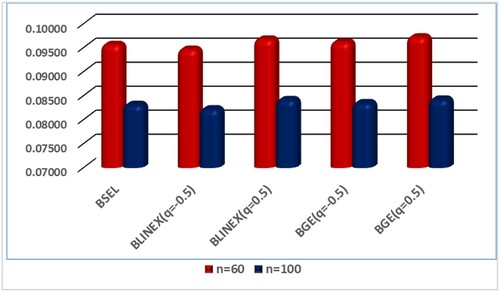
Figure 3. The MSE of Shannon entropy BEs based on BLINEX and BGE loss functions.
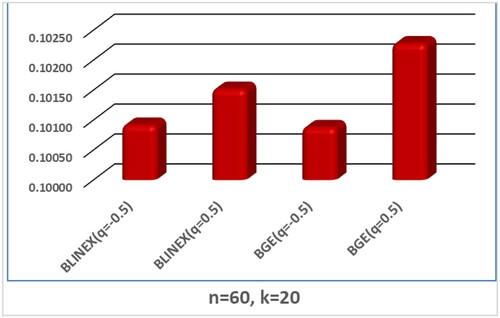
Figure 4. The MSE of Shannon entropy estimation under different values of k at n = 60.
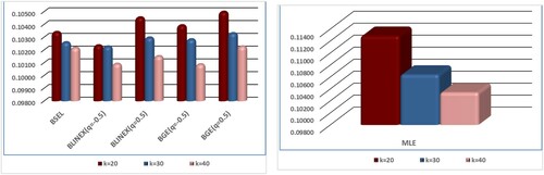
Figure 5. The MSE of Shannon entropy estimates at ( and
), (
and
) and (
and
) for
.
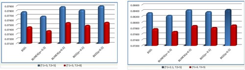
Figure 6. MCMC plots at .
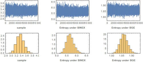
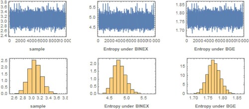
Figures and display a trace plot of the Shannon entropy for different loss functions with iteration numbers (1000) for and
and for
, respectively. The estimations show that all of the generated posteriors fit the theoretical posterior density functions very well, and it is clear that a large MCMC loop produces similar and more efficient outcomes. These plots resemble a horizontal band with no long upward or downward trends, which are convergence markers.
Figure 7. MCMC plots at .
6. Real life data
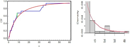
To demonstrate the proposed methodologies, we look at an application to two real data sets in this section. Nelson [Citation35] provided these statistics, which Abd Ellah [Citation36] discussed. The first data set was obtained at a voltage of 34 kV (minutes), and these data represent the time it takes for an insulating fluid between electrodes to break down (minutes). The 19 times to breakdown are recorded as
Abd Ellah [Citation36] used the Kolmogorov–Smirnov test to evaluate the correctness of the fitted model where the P-value = 0.749683 and statistic value is 0.147477. The estimated pdf and cdf are represented in Figure .
Figure 8. Estimated pdf and cdf of the Lo distribution for first data.
Now we will look at what happens if the data are censored. From the uncensored data set, we generate six artificially UHCD sets as follows:
Case 1: in this situation
.
Case 2: in this situation
.
Case 3: in this situation
.
Case 4: in this situation
.
Case 5: in this situation
.
Case 6: in this situation
.
In these cases, we used ML and a Bayesian estimate of Shannon entropy. We used 11,000 MCMC sample and discarded the first 1000 values as “burn-in” under balanced loss functions (BSLE, BLINEX, BGE) when . Since we do not know anything about the priors, we use a non-informative prior to compute the Bayes estimators, thus we choose
and
, as shown in Table .
Table 3. Shannon entropy estimators for first data.
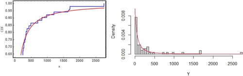
The second data were obtained from a meteorological study by Simpson [Citation37]. The data represent radar-evaluated rainfall from 52 south Florida cumulus clouds. This data set was successfully fitted for the Lo distribution using the Kolmogorov–Smirnov test with a statistic value of 0.0825474 and a P-value . The estimated pdf and cdf are represented in Figure .
Figure 9. Estimated pdf and cdf of Lo distribution for second data.
Now we will look at what happens if the data are censored. From the uncensored data set, we generate six artificially UHCD sets as follows:
Case 1: in this situation
.
Case 2: in this situation
.
Case 3: in this situation
.
Case 4: in this situation
.
Case 5: in this situation
.
Case 6: in this situation
.
In these cases, we used ML and a Bayesian estimate of Shannon entropy. We used 11,000 MCMC sample and discarded the first 1000 values as “burn-in” under balanced loss functions (BSLE, BLINEX, BGE) when . Since we do not know anything about the priors, we use a non-informative prior to compute the Bayes estimators, thus we choose
and
, as shown in Table . Figures and show the trace plot and histogram of the first 1000 MCMC outputs for posterior distribution of
for case 1 based on UHCS for first real and second real data respectively.
Figure 10. The trace plot and histogram of posterior samples for case 1 of UHCS for the first real data.
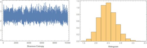
Figure 11. The trace plot and histogram of posterior samples for case 1 of UHCS for the second real data.
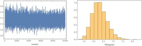
Table 4. Shannon entropy estimators for second data.
We note from the study of these applications in Tables and the amount of data obtained in Bayesian estimation is larger than at MLE because the uncertainty in the case of Bayesian is less than the uncertainty in MLE.
The BE based on BLINEX and BGE loss functions at has a large amount of data where at
has a less amount of data because it has a large amount of uncertainty and this is the same result in simulation study.
7. Conclusion and summary
In this paper, the maximum likelihood and Bayesian estimation of Shannon entropy for Lo distribution under UHCS are considered. The Bayesian estimate of Shannon entropy for Lo distribution is obtained based on balanced loss functions (BSEL, BLINEX, BGE). The MCMC method is employed to calculate the Bayesian estimator of Shannon entropy under BSEL, BLINEX, BGE in terms of their mean squared error. Application to real data is provided.
Regarding the simulation results, we conclude that the mean squared error of ML and Bayesian estimates of the Shannon entropy decrease as the sample size increases. The entropy estimates via BLNIEX and BGE loss functions are chosen over the others at , allowing for more information. The MLE and BE of Shannon entropy are preferred above the others when
, providing more information for fixed values of
. The BE has a greater amount of information than MLE since the uncertainty in BE is lower. In future work, one might study the challenge of estimating other measures of uncertainty using the E-Bayesian approach under UHCS. In this study, we used the MCMC method to calculate the Bayesian estimator of Shannon entropy under BSEL, BLINEX, BGE. Other approaches, such as Tierney–Kadane approximation and Lindley approximation will be used along with the MCMC approach under BSEL, BLINEX, BGE or another types of loss functions.
Acknowledgements
The authors would like to express their gratitude to the editor and the anonymous referees for their insightful and constructive remarks, which have significantly improve the paper's substance.
Disclosure statement
No potential conflict of interest was reported by the author(s).
Correction Statement
This article has been republished with minor changes. These changes do not impact the academic content of the article.
Additional information
Funding
References
- Epstein B. Truncated life tests in exponential case. Ann Math Stat. 1954;25:555–564. doi:https://doi.org/10.1214/aoms/1177728723.
- Childs A, Chandrasekar B, Balakrishnan N, et al. Exact likelihood inference based on type-I and type-II hybrid censored samples from the exponential distribution. Ann Inst Stat Math. 2003;55:319–330. doi:https://doi.org/10.1007/BF02530502.
- Chandrasekar B, Childs A, Balakrishnan N. Exact likelihood inference for the exponential distribution under generalized type-I and type-II hybrid censoring. Nav Res Logist. 2004;51(7):994–1004. doi:https://doi.org/10.1002/nav.20038.
- Balakrishnan N, Rasouli A, Farsipour AS, et al. Exact likelihood inference based on an unified hybrid censoring sample from the exponential distribution. J Stat Comput Simul. 2008;78:475–488. doi:https://doi.org/10.1080/00949650601158336.
- Ateya FS. Estimation under inverse Weibull distribution based on Balakrishnan's unified hybrid censored scheme. Commun Stat Simul Comput. 2017;46(5):3645–3666. doi:https://doi.org/10.1080/03610918.2015.1099666.
- Shannon CE. A mathematical theory of communication. Bell Syst Tech. 1948;27(3):379–432. doi:https://doi.org/10.1002/j.1538-7305.1948.tb01338.
- Cover TM, Thomas JA. Elements of information theory. Hoboken (NJ): Wiley; 2005.
- Eun SK, Jung NS, Lee JJ, et al. Uncertainty of agricultural product prices by information entropy model using probability distribution for monthly prices. Korean J Int Agric. 2012;54(2):7–14. doi:https://doi.org/10.5389/KSAE.2012.54.2.007.
- Chang DE, Ha KR, Jun HD, et al. Determination of optimal pressure monitoring locations of water distribution systems using entropy theory and genetic algorithm. J Korean Soc Water Wastewater. 2009;42(7):537–546. www.jksww.or.kr/journal/article.php?code=18843.
- Mamourian M, Shirvan KM, Ellahi R, et al. Optimization of mixed convection heat transfer with entropy generation in a wavy surface square lid-driven cavity by means of Taguchi approach. Int J Heat Mass Transfer. 2016;102:544–554. doi:https://doi.org/10.1016/j.ijheatmasstransfer.2016.06.056.
- Shehzad N, Zeeshan A, Ellahi R, et al. Modelling study on internal energy loss due to entropy generation for non-Darcy Poiseuille flow of silver-water nanofluid: an application of purification. Entropy. 2018;20(11):8–51. doi:https://doi.org/10.3390/e20110851.
- Ellahi R, Alamri SZ, Basit A, et al. Effects of MHD and slip on heat transfer boundary layer flow over a moving plate based on specific entropy generation. J Taibah Univ Sci. 2018;12(4):476–482. doi:https://doi.org/10.1080/16583655.2018.1483795.
- Rass S, König S. Password security as a game of entropies. Entropy. 2018;20(5):312. doi:https://doi.org/10.3390/e20050312.
- Morabbi H, Razmkhah M. Entropy of hybrid censoring schemes. J Stat Res Iran. 2009;6:161–176. doi:https://doi.org/10.18869/acadpub.jsri.6.2.161.
- Abo-Eleneen ZA. The entropy of progressively censored samples. Entropy. 2011;13(2):437–449. doi:https://doi.org/10.3390/e13020437.
- Cho Y, Sun H, Lee K, et al. An estimation of the entropy for a Rayleigh distribution based on doubly generalized type- II hybrid censored samples. Entropy. 2014;16:3655–3669. doi:https://doi.org/10.3390/e16073655.
- Liu S, Gui W. Estimating the entropy for Lomax distribution based on generalized progressively hybrid censoring. Symmetry. 2019;11(10):1219. doi:https://doi.org/10.3390/sym11101219.
- Hassan AS, Zaky AN. Estimation of entropy for inverse Weibull distribution under multiple censored data. J Taibah Univ Sci. 2019;13:331–337. doi:https://doi.org/10.1080/16583655.2019.1576493.
- Yu J, Gui W, Shan Y, et al. Statistical inference on the Shannon entropy of inverse Weibull distribution under the progressive first-failure censoring. Entropy. 2019;21(12):1209. doi:https://doi.org/10.3390/e21121209.
- Bantan RAR, Elgarhy M, Chesneau C, et al. Estimation of entropy for inverse Lomax distribution under multiple censored data. Entropy. 2020;22(6):601. doi:https://doi.org/10.3390/e22060601.
- Hassan AS, Al-Ghamdi AN. Optimum step stress accelerated life testing for Lomax distribution. J Appl Sci Res. 2009;5:2153–2164.
- Lomax KS. Business failures: another example of the analysis of failure data. J Am Stat Assoc. 1954;49(268):847–852. doi:https://doi.org/10.1080/01621459.1954.10501239.
- Harris CM. The Pareto distribution as a queue service discipline. Oper Res. 1968;16(2):307–313. doi:https://doi.org/10.1287/opre.16.2.307.
- Atkinson AB, Harrison AJ, James A, et al. Distribution of personal wealth in Britain. Cambridge: Cambridge University Press; 1978.
- Campbell G, Ratnaparkhi MV. An application of Lomax distributions in receiver operating characteristic (roc) curve analysis. Commun Stat Theory Methods. 1993;22(6):1681–1687. doi:https://doi.org/10.1080/03610929308831110.
- Hassan AS, Assar SM, Shelbaia A, et al. Optimum step-stress accelerated life test plan for Lomax distribution with an adaptive type-II progressive hybrid censoring. J Adv Math Compute Sci. 2016;13(2):1–19. doi:https://doi.org/10.9734/BJMCS/2016/21964.
- Balakrishnan N, Ahsanullah M. Relations for single and product moments of record values from Lomax distribution. Sankhya A, Series B. 1994;56(2):140–146. https://www.jstor.org/stable/25052832.
- Okasha HM. E-Bayesian estimation for the Lomax distribution based on type-II censored data. J Egypt Math Soc. 2014;22:489–495. doi:https://doi.org/10.1016/j.joems.2013.12.009.
- Singh SK, Singh U, Yadav AS, et al. Bayesian estimation of Lomax distribution under type-II hybrid censored data using Lindley's approximation method. Int J Data Sci. 2017;2:352–368. doi:https://doi.org/10.1504/IJDS.2017.10009048.
- Ahmadini AAH, Hassan AS, Zaky AN, et al. Bayesian inference of dynamic cumulative residual entropy from Pareto II distribution with application to COVID-19. AIMS Math. 2020;6(3):2196–2216. doi:https://doi.org/10.3934/math.2021133.
- Al-Babtain AA, Hassan AS, Zaky AN, et al. Dynamic cumulative residual Rényi entropy for Lomax distribution: Bayesian and non-Bayesian methods. AIMS Math. 2021;6(4):3889–3914. doi:https://doi.org/10.3934/math.2021231.
- Hassan AS, Zaky AN. Entropy Bayesian estimation for Lomax distribution based on record. Thail Stat. 2021;19(1):95–114.
- Zellner A. Bayesian and non-Bayesian estimate using balanced loss functions. In: Berger JO, Gupta SS, editors. Statistical decision theory and related topics V. New York: Springer-Verlag; 1994. p. 337–390.
- Metropolis N, Rosenbluth AW, Rosenbluth MN, et al. Equations of state calculations by fast computing machines. J Chem Phys. 1953;21:1087–1091. doi:https://doi.org/10.1063/1.1699114.
- Nelson WB. Applied life data analysis. New York: John Wiley and Sons; 1982.
- Abd Ellah AH. Comparison of estimates using record statistics from Lomax model: Bayesian and non Bayesian approaches. J Stat Res Iran. 2006;3(2):139–158. doi:https://doi.org/10.18869/acadpub.jsri.3.2.139.
- Simpson J. Use of the gamma distribution in single-cloud rainfall analysis. Mon Weather Rev. 1972;100:309–312. doi:https://doi.org/10.1175/1520-0493(1972)100<0309:UOTGDI>2.3.CO;2.