An analysis of the classical gambler's ruin problem through multiple devices variation

Abstract

In this study, we propose a variant of classic 2-player ruin's problem. We advocate the use of simultaneous operation of multiple devices to conclude upon the game. The suggested scheme is rigorously analysed and shown to be balancing the game duration to a notable extend in order to achieve desirable features of giving both players opportunity to comeback as well as avoiding the stalemates. The proposed scheme, at first, mathematically elaborated by providing general expressions of the ruin probability, the ruin time, the conditional ruin time and the variance of the game. The foundational blocks of the devised game are tested and validated in-concordance with the various pre-fixation adapted by Stern (1975) and Samuels (1975). In pursuit of the objectives, the mathematical outcomes are rigorously verified by simulating various adaptations under diverse parametric settings.

Keywords:

• Classical gambler's ruin problem
• ruin probability
• ruin time
• conditional ruin time
• simultaneous operation

1. Introduction

The classic gambler's ruin problem was introduced by Pascal – an influential mathematician of his era (seventeenth century); see for example [1]. The significance of the ruin problem can be seen throughout the literature. Despite such a long history of the gambler's ruin problem, it is still a problem of wide interests, see for examples, Morrow [2], Hussain et al. [3], Perotto et al. [4] and Hussain et al. [5]. To further appreciate the extended applicability of the concept in multidisciplinary research, see [6,7] in the field of applied mathematics, [8] in epidemiology, [9] in physics, [10] in the field of hydrology, [11] in quantum mechanics, [12] in biological sciences and [13] in business risk assessment.

In its simplest form, the classic ruin problem starts with two players, playing with k and a−k amount of stakes, say dollars, where a represents the total capital involved in the game. Further, before the start, one of the players either win a predefined amount of capital with probability, p or lose with probability, 1−p = q and vice versa for the other player. The main interest lies in strategizing the probability of ruin/raising and the anticipation of expected ruin time of the game. The ruin probability, say ${\mu }_k$, of absorption of zero and the time remaining in the game, say $T_k$, are given by Feller [14], such as: (1) ${\mu }_k=\{\begin{array}{ll}{\displaystyle \frac{a-k}{a}};& q=p\\ {\displaystyle \frac{(r{)}^k-(r{)}^a}{1-(r{)}^a}};& q\ne p,\end{array}$(1) and, (2) $E(T_k)=\{\begin{array}{ll}{\displaystyle \frac{k(a-k)}{2p}};& q=p\\ {\displaystyle \frac{1}{q-p}}({\displaystyle \frac{a((r{)}^k-1)}{1-(r{)}^a}}+k);& q\ne p,\end{array}$(2) where $r=\frac{q}{p}$. The above expressions are valid for both cases, i.e. when there is no involvement of ties, i.e. p + q = 1 and with the ties, i.e. p + q<1.

For conditional expectations, Stern [15] provided the expressions of $E_k$ and $F_k$, indicating the expected steps a player has to stop the game while suffering from complete loss or gaining maximum fortune, respectively. The general expressions are given as: (3) $E_k=\{\begin{array}{ll}{\displaystyle \frac{k(2a-k)}{3}};& q=p\\ {\displaystyle \frac{(p-q{)}^{-1}}{r^k-r^a}}(k(r^k+r^a)\\ +2a\left({\displaystyle \frac{r^{k+a}-r^a}{1-r^a}}\right));& q\ne p,\end{array}$(3) and, (4) $F_k=\{\begin{array}{ll}{\displaystyle \frac{1}{3}}(a^2-k^2);& q=p\\ {\displaystyle \frac{(p-q{)}^{-1}}{1-r^k}}((a-k)(r^k+1)\\ +2a\left({\displaystyle \frac{r^k-r^a}{r^a-1}}\right));& q\ne p.\end{array}$(4) For the variance of ruin time of the classic 2-player problem, Bach [16] provided the following expression for the symmetric game as: (5) $Var(T_k)=\frac{k(a-k)}{3}(k^2+(a-k{)}^2-2).$(5) By allowing the tie in a single trial, Andel and Hudecova [17] further derived the expression of the variance of ruin time, when p = q as: (6) $Var(T_k)=\frac{k(a-k)}{12p^2}(k^2+(a-k{)}^2+1-6p).$(6) For the asymmetric game, Andel and Hudecova [17] derived the following expression for both situations, i.e. either ties are involved or not in the game as: (7) $\begin{array}{rl}& Var(T_k)\\ & =-\frac{a^2{r}^{2k}}{p^2(r-1{)}^2(r^a-1{)}^2}+\frac{4ak{r}^k}{p^2(r-1{)}^2(r^a-1)}\\ & +\frac{\begin{array}{c}a{r}^k((p(r-1{)}^2-r-1)(r^a-1)\\ -a(r-1)(3r^a-1))\end{array}}{p^2(r-1{)}^3(r^a-1{)}^2}\\ & -\frac{k(p(r-1{)}^2-r-1)}{p^2(r-1{)}^3}\\ & +\frac{\begin{array}{c}a((1-3a)r^a+(1+3a)r^{a+1}\\ -p(r-1{)}^2(r^a-1)-r-1)\end{array}}{p^2(r-1{)}^3(r^a-1{)}^2},\end{array}$(7) where, $r=q/p$.

In literature, many researchers have been proposed variants of the classic ruin problem. For example, Kmet and Petkovsek [18] and Ethier [19] extended the game for the case of infinite stakes involved. Lefebvre [20] and El-Shehawey [21] introduced a novel mechanism of taking current fortune of the players into account while quantifying the probabilities. Moreover, Lengyel [22] extended this classic game by allowing the occurrence of ties. Harper and Ross [23] involved a variable reward for success and failure in the classic game. Another variant with multidimensional generalized gambler's ruin problem can be seen in [24]. Hussain et al. [3] and Hussain and Cheema [25] solved this game when decision based on successive events. Most recently, Perotto et al. [4] suggested the optimal rule to quit the game with unknown probabilities.

In this article, we propose a novel amendment in the conduction of classical 2-player game. We argue the introduction of multiple devices simultaneously to decide on players' gain or loss. It is proved, mathematically and through rigorous simulation, that with the application of devised strategy, the ruin time of the game increased geometrically with respect to the number of devices. This line of operation is expected to provide both opponents an enhanced chance of making a come back. We offer general expressions for the quantification of ruin probabilities, the ruin time and the conditional of ruin time and the variance of desired game plan. It is important to note that the classical 2-player ruin game stays as a sub case of the proposed scheme. The proposed portfolio is thoroughly studied through simulation while considering various parametric settings.

In the next section (Section 2), we provide the mathematical developments for the ruin probabilities, expected and conditionally expected ruin times under the proposed structure and variance of the game. The performance evaluation is measured through numerical findings of the proposed strategy and then verified through a simulation study in Section 3. Finally, we summarize the research work in Section 4.

2. Mathematical developments

In this section, we aim at deriving the mathematical expressions for the ruin probability, the ruin time, the conditional expectations with respect to an individual's ruin time and variance of the game. The afore-mentioned statistics are calculated under the proposed scheme, i.e. by involving c simultaneous devices in the play. Thus, after each round of the game, the gambler either wins predefined units of the capital with probability $p^c$ or loses with probability $q^c$. Besides that, one may appreciate that the proposed strategy takes the probability of ties into account automatically, i.e. ($1-(p^c+q^c)$). In this article, we advocate the case of “no stake exchanged” in case of ties. For demonstration purposes, we provide results for the proposed scheme, when only two devices (most practical) are involved in the game, i.e. c = 2. It can be noted that Table 1 can be extended for the c number of devices involved in the game for the decision of a play. In the next lines, we derive the required expressions for the proposed scheme. For simplicity, we initiate our calculations for the most practical and simple case, i.e. c = 2. The general expressions are also provided.

Table 1. Absorption probabilities, the ruin time, conditional ruin times and variance of the game for c = 2.

p	k	a	${\mu }_k$	$E(T_k)$	$E_k$	$F_k$	$Var(k)$
	1	20	0.2899	44.00	3.33	60.61	879.74
	5	20	0.0020	49.87	16.67	49.93	252.07
0.65	10	20	0.0000	33.33	33.33	33.33	168.50
	15	20	0.0000	16.67	49.93	16.67	84.26
	19	20	0.0000	3.34	60.61	3.33	16.86
	1	20	0.5244	53.21	6.25	104.97	3270.89
	5	20	0.0396	88.80	31.24	91.17	1665.42
0.58	10	20	0.0016	62.31	62.31	62.31	1161.24
	15	20	0.0001	31.25	91.17	31.24	592.75
	19	20	0.0000	6.25	104.97	6.25	118.85
	1	20	0.7846	55.12	15.51	199.45	9573.60
	5	20	0.2950	151.67	74.85	183.82	12988.86
0.53	10	20	0.0830	139.02	139.02	139.02	10785.82
	15	20	0.0192	76.94	183.82	74.85	7190.80
	19	20	0.0022	15.92	199.95	15.51	1680.53
	1	20	0.9500	38.00	26.00	266.00	9158
	5	20	0.7500	150.00	116.67	250.00	24950
0.50	10	20	0.5000	200.00	200.00	200.00	26,600
	15	20	0.2500	150.00	250.00	116.67	24,950
	19	20	0.0500	38.00	266.00	26.00	9158

2.1. The ruin probabilities

Let, ${\mu }_k$ be the ruin probability of the player (gambler), playing with k amount of capital. Then the law of total probability, when c = 2 can be written in the following difference equation: (8) ${\mu }_k={\mu }_{k+1}(p^2)+{\mu }_k(1-p^2-q^2)+{\mu }_{k-1}(q^2).$(8) For the case of symmetric game, i.e. when both players are playing with equal probabilities of win. Equation (8(8) ${\mu }_k={\mu }_{k+1}(p^2)+{\mu }_k(1-p^2-q^2)+{\mu }_{k-1}(q^2).$(8) ) has two similar roots, i.e. ${\lambda }_1={\lambda }_2$, and we get the following general solution: (9) ${\mu }_k=C_0+C_{1}k,$(9) where, $C_0$ and $C_1$ are two constants. By using two boundary conditions driven by two extremes, i.e. ${\mu }_0=1$ and ${\mu }_a=0$, we get $C_0=1$ and $C_1=-1/a$. Hence, Equation (9(9) ${\mu }_k=C_0+C_{1}k,$(9) ) reduces to: (10) ${\mu }_k=\frac{a-k}{a}.$(10) For c = 3, it remains verifiable that the difference equation will be: ${\mu }_k={\mu }_{k+1}(p^3)+{\mu }_k(1-p^3+q^3)+{\mu }_{k-1}(q^3)$, and for symmetric case, this gives the general solution as similar to Equation (9(9) ${\mu }_k=C_0+C_{1}k,$(9) ). After simplification, we get same ruin probability as we had with c = 2. Hence, for symmetric case, the ruin probability does not depend on the number of devices, therefore, the expression given in Equation (10(10) ${\mu }_k=\frac{a-k}{a}.$(10) ) is valid for any c. For the asymmetric case, i.e. when both players are playing with unequal probabilities of win. In this case, Equation (8(8) ${\mu }_k={\mu }_{k+1}(p^2)+{\mu }_k(1-p^2-q^2)+{\mu }_{k-1}(q^2).$(8) ) satisfies the following difference equation: $(p^2){\mu }_{k+1}-(p^2+q^2){\mu }_k+q^2{\mu }_{k-1}=0.$The above equation gives two different roots, i.e. ${\lambda }_1=1$ and ${\lambda }_2=\frac{q^2}{p^2}$, and we get the following general solution: ${\mu }_k=C_0{\lambda }_1^k+C_1{\lambda }_2^k.$The values of the two constants after using the boundary conditions (mentioned earlier) are: $C_0=\frac{-r^a}{1-r^a}$ and $C_1=\frac{1}{1-r^t}$, where, $r=\frac{q^2}{p^2}$. The general solution after simplification is: (11) ${\mu }_k=\frac{{\left(\frac{q^2}{p^2}\right)}^k-{\left(\frac{q^2}{p^2}\right)}^a}{1-{\left(\frac{q^2}{p^2}\right)}^a}.$(11) For c = 3, Equation (8(8) ${\mu }_k={\mu }_{k+1}(p^2)+{\mu }_k(1-p^2-q^2)+{\mu }_{k-1}(q^2).$(8) ) gives the following difference equation: $(p^3){\mu }_{k+1}-(p^3+q^3){\mu }_k+q^3{\mu }_{k-1}=0,$and by using similar approach as mentioned above, we get the following solution: (12) ${\mu }_k=\frac{{\left(\frac{q^3}{p^3}\right)}^k-{\left(\frac{q^3}{p^3}\right)}^a}{1-{\left(\frac{q^3}{p^3}\right)}^a}.$(12) Hence, the ruin probabilities given in Equations (11(11) ${\mu }_k=\frac{{\left(\frac{q^2}{p^2}\right)}^k-{\left(\frac{q^2}{p^2}\right)}^a}{1-{\left(\frac{q^2}{p^2}\right)}^a}.$(11) ) and (12(12) ${\mu }_k=\frac{{\left(\frac{q^3}{p^3}\right)}^k-{\left(\frac{q^3}{p^3}\right)}^a}{1-{\left(\frac{q^3}{p^3}\right)}^a}.$(12) ) are generalized for any c as: ${\mu }_k=\frac{{\left(\frac{q^c}{p^c}\right)}^k-{\left(\frac{q^c}{p^c}\right)}^a}{1-{\left(\frac{q^c}{p^c}\right)}^a}.$

2.2. The expected ruin time of the game

The general expression for the calculation of expected ruin time can be written as: (13) $E(T_k)=\sum _{n=0}^{\mathrm{\infty }}nP(n|k),$(13) where n is the required number of trials to complete the game and k is the initial amount of gambler. By employing our scheme, i.e. c = 2 and under the law of total probability, the above expression is simplified in the following form: $\begin{array}{rl}P(n|k)& =P(n-1|k+1)(p^2)+P(n-1|k)(1-p^2-q^2)\\ & +P(n-1|k-1)(q^2).\end{array}$After using expectation operation and $E(T_k)=d_k$ (say) for simplicity, the above equation reduces to: (14) $(p^2)d_{k+1}+(2pq-1)d_k+q^2{d}_{k-1}=-1.$(14) For the case of symmetric game, i.e. $p=q=\frac{1}{2}$, the difference Equation (14(14) $(p^2)d_{k+1}+(2pq-1)d_k+q^2{d}_{k-1}=-1.$(14) ) can be simplified as: $d_{k+1}-2d_k+d_{k-1}=-4.$Under the boundary conditions such that $d_0=d_a=0$, the complementary solution is $d_k=A_1+A_{2}k$, where $A_1$ and $A_2$ are constants and the particular solution remains $-2k^2$. Thus the general solution is: (15) $d_k=2k(a-k).$(15) Next, for c = 3, we can write the following difference equation as: $\begin{array}{rl}P(n|k)& =P(n-1|k+1)(p^3)+P(n-1|k)(1-p^3-q^3)\\ & +P(n-1|k-1)(q^3).\end{array}$After solving in similar fashion, we get the final solution as: $d_k=4k(a-k).$Therefore, the solution can be generalized for c number of simultaneous devices as: $E(T_k)=d_k=2^{c-1}k(a-k).$Moreover, for a fixed amount of stakes, the expected ruin time of the game increases with respect to the number of devices increased.

For the asymmetric case, i.e. $p\ne q$, the complementary solution of Equation (14(14) $(p^2)d_{k+1}+(2pq-1)d_k+q^2{d}_{k-1}=-1.$(14) ) satisfying the above given boundary conditions is: $B_1+(\frac{q^2}{p^2}{)}^k{B}_2$, where $B_1$ and $B_2$ are constants. Similarly, the particular solution is given as $\frac{k}{q^2-p^2}$. So, the general solution can be written as: $d_k=B_1+{\left(\frac{q^2}{p^2}\right)}^k{B}_2+\frac{k}{q^2-p^2}.$By using the above-mentioned two boundary conditions, we can determine the two constant in the above equation as: $B_1=\frac{-a}{(q^2-p^2)(1-r^2)}$ and $B_2=\frac{a}{(q^2-p^2)(1-r^2)}$, where, $r=\frac{q}{p}$. This will lead the final solution after some simplification as: (16) $d_k=\frac{1}{q^2-p^2}(\frac{a((r^2{)}^k-1)}{1-(r^2{)}^a}+k).$(16) In the case of c = 3, the ruin time is calculated in similar fashion and we get the following result: $d_k=\frac{1}{q^3-p^3}(\frac{a((r^3{)}^k-1)}{1-(r^3{)}^a}+k).$Hence, for generalization, the expected ruin time is written for any c as: $d_k=\frac{1}{q^c-p^c}(\frac{a((r^c{)}^k-1)}{1-(r^c{)}^a}+k).$

2.3. The conditional ruin time of the game

Let us define $E_k$ and $F_k$ to be the conditional expectations for the number of plays conditioning on the notion that the game will stop with ruin of the player playing with k amount of stake, or with winning of maximum fortunes involved in the game, respectively. The ruin time of the game while considering the conditional expectations is calculable as: $d_k={\mu }_k{E}_k+(1-{\mu }_k)F_k.$We consider, ${\mu }_k{E}_k=d_{k,0}$ and $(1-{\mu }_k)F_k=d_{k,a}$, then the above equation can be written as: $d_k=d_{k,0}+d_{k,a},$where $d_{k,0}$ represents the expected ruin time of the game conditional upon the player finishes at “zero” stake and $d_{k,a}$ is the expected ruin time of the game given that player enjoys maximum fortunes. The probability of ruin, ${\mu }_k$, involving the number of plays can be written as: ${\mu }_k=\sum _{n=1}^{\mathrm{\infty }}{\mu }_{k,n}.$Then the expression of conditional ruin time of the game given that the player playing with k stakes, is written as: (17) $d_{k,0}=\sum _{n=1}^{\mathrm{\infty }}n{\mu }_{k,n}.$(17) The conditional expected ruin time of the game, given that the player enjoys the maximum stakes involved in the game, that is, $d_{k,a}$ can be derived through the expression such as $d_{k,a}=d_{a-k,0}$. In the next lines, we derive the solutions for the expression given in above equation for both cases, i.e. symmetric and asymmetric.

For the symmetric case, i.e. both players are playing with equal probabilities of win. The $d_{k,0}$ of Equation (17(17) $d_{k,0}=\sum _{n=1}^{\mathrm{\infty }}n{\mu }_{k,n}.$(17) ) satisfies the following difference equation: (18) $d_{k+1,0}-2d_{k,0}+d_{k-1,0}=-4{\mu }_k.$(18) By using the value of ${\mu }_k$ given in Equation (10(10) ${\mu }_k=\frac{a-k}{a}.$(10) ) and the boundary conditions, i.e. $d_{0,0}=d_{a,0}=0$, a complementary solution of Equation (18(18) $d_{k+1,0}-2d_{k,0}+d_{k-1,0}=-4{\mu }_k.$(18) ) is $C_1+C_{2}k$, where $C_1$ and $C_2$ are constants. Similarly, the particular solution is given as $2k^2(\frac{k}{3a}-1)$. Therefore the unique solution of the inhomogeneous equation [Equation (18(18) $d_{k+1,0}-2d_{k,0}+d_{k-1,0}=-4{\mu }_k.$(18) )] satisfying the boundary conditions can be given as: $d_{k,0}=\frac{2k}{3a}(a-k)(2a-k),$and hence, (19) $E_k=\frac{2k}{3}(2a-k).$(19) Next, by replacing k with a−k in the expression of $d_{k,0}$, we attain the conditional expected ruin time of the game given that the gambler wins the whole stakes, $F_k$, as follows: (20) $F_k=\frac{2}{3}(a^2-k^2).$(20) The generalization of the expressions of $E_k$ [Equation (19(19) $E_k=\frac{2k}{3}(2a-k).$(19) )] and $F_k$ [Equation (20(20) $F_k=\frac{2}{3}(a^2-k^2).$(20) )], for “c” number of devices can be written as: $E_k=\frac{2^{c-1}k}{3}(2a-k),$and $F_k=\frac{2^{c-1}}{3}(a^2-k^2).$Both conditional expectations remain the function of the number of devices for a constant amount of stakes.

For the asymmetric case, i.e. both players are playing with unequal probabilities of win. Under this condition, we get the resultant difference equation in the following form: $p^2{d}_{k+1,0}-(2pq-1)d_{k,0}+q^2{d}_{k-1,0}=-{\mu }_k.$We proceed by using probability generating function and value of ${\mu }_k$ given in Equation (12(12) ${\mu }_k=\frac{{\left(\frac{q^3}{p^3}\right)}^k-{\left(\frac{q^3}{p^3}\right)}^a}{1-{\left(\frac{q^3}{p^3}\right)}^a}.$(12) ) while satisfying the above-mentioned boundary conditions. The probability generating function is given as: $G_n(s)=\sum _{n=0}^{\mathrm{\infty }}{p}_n{s}^n,$which simplifies as: $G_k(s)=\sum _{n=0}^{\mathrm{\infty }}{\mu }_{k,n}{s}^n,$where s is a dummy variable indicating the nature of step-function. By using difference equation, the probability generating function simplifies for the case of c = 2 as: (21) $G_k(s)=\frac{{\lambda }_1^a(s){\lambda }_2^k(s)-{\lambda }_1^k(s){\lambda }_2^a(s)}{{\lambda }_1^a(s)-{\lambda }_2^a(s)},$(21) where, ${\lambda }_1(s)=\frac{(1-2pqs)+\sqrt{1-4pqs}}{2p^{2}s},$and, ${\lambda }_2(s)=\frac{(1-2pqs)-\sqrt{1-4pqs}}{2p^{2}s}.$Next, we proceed by applying usual operations to solve expected number of steps through probability generating function and document them for p>q and p<q. The expected number of steps when p>q are attained by differentiating $G_k(s)$ with respect to s and putting s = 1, such that $d_{k,0}=G_k^{\prime }(1)$. By following this line of operations, we observe ${\lambda }_1(1)=1$, ${\lambda }_1^{\prime }(1)=(q-p{)}^{-1}$, ${\lambda }_2(1)=\frac{q^2}{p^2}=r^2$, ${\lambda }_2^{\prime }(1)=\frac{q^2}{p^2}(p-q{)}^{-1}=r^2(p-q{)}^{-1}$. For p<q, the documented results hold exactly same with interchanged subscript, 1 and 2 in Equation (21(21) $G_k(s)=\frac{{\lambda }_1^a(s){\lambda }_2^k(s)-{\lambda }_1^k(s){\lambda }_2^a(s)}{{\lambda }_1^a(s)-{\lambda }_2^a(s)},$(21) ). Thus, the expected duration of the game for ruined player, $d_{k,0}$ is solved as: $\begin{array}{rl}{d}_{k,0}& =\frac{(p-q{)}^{-1}}{1-(r^2{)}^a}\\ & \times (k((r^2{)}^k+(r^2{)}^a)+2a\left(\frac{(r^2{)}^{k+a}-(r^2{)}^a}{1-(r^2{)}^a}\right)).\end{array}$Since, ${\mu }_k{E}_k=d_{k,0}$, we get $E_k$ as: (22) $\begin{array}{rl}{E}_k& =\frac{(p-q{)}^{-1}}{(r^2{)}^k-(r^2{)}^a}\\ & \times (k((r^2{)}^k+(r^2{)}^a)+2a\left(\frac{(r^2{)}^{k+a}-(r^2{)}^a}{1-(r^2{)}^a}\right)).\end{array}$(22) As, $d_{k,a}=d_{a-k,0}$, therefore $\begin{array}{rl}{d}_{k,a}& =\frac{(q-p{)}^{-1}}{(r^2{)}^a-1}\\ & \times ((a-k)((r^2{)}^k+1)+2a\left(\frac{(r^2{)}^k-(r^2{)}^a}{(r^2{)}^a-1}\right)).\end{array}$The expression of $F_k$ is provided as: (23) $\begin{array}{rl}{F}_k& =\frac{(p-q{)}^{-1}}{1-(r^2{)}^k}\\ & \times ((a-k)((r^2{)}^k+1)+2a\left(\frac{(r^2{)}^k-(r^2{)}^a}{(r^2{)}^a-1}\right)).\end{array}$(23) The general expressions for $E_k$ and $F_k$ while using c number of devices, can be achieved by replacing $r^2$ with $r^c$ in the expressions of Equations (22(22) $\begin{array}{rl}{E}_k& =\frac{(p-q{)}^{-1}}{(r^2{)}^k-(r^2{)}^a}\\ & \times (k((r^2{)}^k+(r^2{)}^a)+2a\left(\frac{(r^2{)}^{k+a}-(r^2{)}^a}{1-(r^2{)}^a}\right)).\end{array}$(22) ) and (23(23) $\begin{array}{rl}{F}_k& =\frac{(p-q{)}^{-1}}{1-(r^2{)}^k}\\ & \times ((a-k)((r^2{)}^k+1)+2a\left(\frac{(r^2{)}^k-(r^2{)}^a}{(r^2{)}^a-1}\right)).\end{array}$(23) ).

2.4. The variance of the game

Let we define $E(T_k^2)=h_k$ and can be expressed as: $E(T_k^2)=h_k=\sum _{n=0}^{\mathrm{\infty }}{n}^{2}P(n|k).$By employing the most practical value of the proposed scheme, i.e. c = 2 and under the law of total probability, the above expression is simplified in the following form: $\begin{array}{rl}{h}_k& =(p^2)h_{k+1}+(2pq)h_k+(q^2)h_{k-1}\\ & +2((p^2)d_{k+1}+(2pq)d_k+(q^2)d_{k-1})+1.\end{array}$After using Equation (14(14) $(p^2)d_{k+1}+(2pq-1)d_k+q^2{d}_{k-1}=-1.$(14) ), the above equation can be reduced as: (24) $h_k=(p^2)h_{k+1}+(2pq)h_k+(q^2)h_{k-1}+2(d_k-1)+1.$(24) For the symmetric case, i.e. $p=q=\frac{1}{2}$ and using Equation (15(15) $d_k=2k(a-k).$(15) ), the above equation can be simplified as: (25) $h_{k+1}-2h_k+h_{k-1}=4-16ak+16k^2.$(25) The complementary solution of Equation (25(25) $h_{k+1}-2h_k+h_{k-1}=4-16ak+16k^2.$(25) ) is $h_k=D_0+D_{1}k$, where $D_0$ and $D_1$ are constants, and the particular solution remains $h_k=D_2{k}^2+D_3{k}^3+D_4{k}^4$, where $D_2=\frac{2}{3}$, $D_3=\frac{-8a}{3}$, and $D_4=\frac{4}{3}$. After using the two boundary conditions, i.e. $h_0=h_a=0$, the general solution of Equation (25(25) $h_{k+1}-2h_k+h_{k-1}=4-16ak+16k^2.$(25) ) is: $h_k=\frac{2a(2a^2-1)k}{3}+\frac{2}{3}{k}^2-\frac{8a{k}^3}{3}+\frac{4k^4}{3}.$We are interested in the variance of the desired game duration as: $Var(T_k)=E(T_k^2)-{(E(T_k))}^2,$ (26) $Var(T_k)=\frac{k(a-k)}{3}(4k^2+4(a-k{)}^2-2).$(26) We can generalize the expression (26(26) $Var(T_k)=\frac{k(a-k)}{3}(4k^2+4(a-k{)}^2-2).$(26) ) for any number of c, as: $Var(T_k)=\frac{k(a-k)}{3}(c{2}^{c-1}{k}^2+c{2}^{c-1}(a-k{)}^2-2).$It remains verifiable for c = 1 with the above-mentioned expression (5(5) $Var(T_k)=\frac{k(a-k)}{3}(k^2+(a-k{)}^2-2).$(5) ) proposed by Bach [16].

For the asymmetric case, i.e. $p\ne q$ and using Equation (16(16) $d_k=\frac{1}{q^2-p^2}(\frac{a((r^2{)}^k-1)}{1-(r^2{)}^a}+k).$(16) ), the above Equation (24(24) $h_k=(p^2)h_{k+1}+(2pq)h_k+(q^2)h_{k-1}+2(d_k-1)+1.$(24) ) can be simplified as: (27) $\begin{array}{rl}& p^2{h}_{k+1}-(1-2pq)h_k+q^2{h}_{k-1}=(1-\frac{2a}{s(1-r^{2a})})\\ & +\left(\frac{2}{s}\right)k+\left(\frac{2a}{s(1-r^{2a})}\right)r^{2k},\end{array}$(27) where, $r=\frac{q}{p}$ and $s=p^2-q^2$. The complementary solution is $h_k=D_5+D_6(r^2{)}^k$, where $D_5$ and $D_6$ are constants and for a particular solution, we take, $h_k=D_{7}k+D_8{k}^2+D_{9}k(r^2{)}^k$. By imposing this in Equation (27(27) $\begin{array}{rl}& p^2{h}_{k+1}-(1-2pq)h_k+q^2{h}_{k-1}=(1-\frac{2a}{s(1-r^{2a})})\\ & +\left(\frac{2}{s}\right)k+\left(\frac{2a}{s(1-r^{2a})}\right)r^{2k},\end{array}$(27) ), we get the following results: $\begin{array}{rl}{D}_7& =\frac{s^2(1-r^{2a})-2sa-(p^2+q^2)(1-r^{2a})}{s^3(1-r^{2a})},\\ D_8& =\frac{1}{s^2}and{D}_9=\frac{-2a}{s^2(1-r^{2a})}.\end{array}$So, the general solution of Equation (27(27) $\begin{array}{rl}& p^2{h}_{k+1}-(1-2pq)h_k+q^2{h}_{k-1}=(1-\frac{2a}{s(1-r^{2a})})\\ & +\left(\frac{2}{s}\right)k+\left(\frac{2a}{s(1-r^{2a})}\right)r^{2k},\end{array}$(27) ) will be in the following form: (28) $h_k=D_5+D_6(r^2{)}^k+D_{7}k+D_8{k}^2+D_{9}k(r^2{)}^k.$(28) After employing the boundary conditions, i.e. $h_0=h_a=0$, we further obtain: $D_5=\frac{2a^2(1+r^{2a})}{s^2(1-r^{2a}{)}^2}-\frac{a(s^2+sa-p^2-q^2)}{s^3(1-r^{2a})},$and, $D_6=\frac{a(s^2+sa-p^2-q^2)}{s^3(1-r^{2a})}-\frac{2a^2(1+r^{2a})}{s^2(1-r^{2a}{)}^2}.$Finally, we have $Var(T_k)=D_5+D_6(r^2{)}^k+D_{7}k+D_8{k}^2+D_{9}k(r^2{)}^k-d_k^2.$ $\begin{array}{rl}Var(T_k)& =\frac{2a^2(1+r^{2a})}{s^2(1-r^{2a}{)}^2}-\frac{a(s^2+sa-p^2-q^2)}{s^3(1-r^{2a})}\\ & +\frac{a(s^2+sa-p^2-q^2)}{s^3(1-r^{2a})}{r}^{2k}\\ & -\frac{2a^2(1+r^{2a})}{s^2(1-r^{2a}{)}^2}{r}^{2k}\\ & +\frac{s^2(1-r^{2a})-2sa-(p^2+q^2)(1-r^{2a})}{s^3(1-r^{2a})}k\\ & +\frac{1}{s^2}{k}^2-\frac{2a}{s^2(1-r^{2a})}k{r}^{2k}\\ & -{(\frac{a(1-r^{2k})}{s(1-r^{2a})}-\frac{k}{s})}^2,\end{array}$which simplify as the following expression: (29) $\begin{array}{rl}Var(T_k)& =\frac{a^2(1-(r^2{)}^{2k})+2a^2(r^2{)}^a(1-(r^2{)}^k)}{s^2{(1-(r^2{)}^a)}^2}\\ & +\frac{k(s^2-p^2-q^2)}{s^3}\\ & +\frac{a(s^2+sa-p^2-q^2)((r^2{)}^k-1)}{s^3(1-(r^2{)}^a)}\\ & -\frac{4ak(r^2{)}^k}{s^2(1-(r^2{)}^a)}.\end{array}$(29)

The generalization of the expression given in Equation (29(29) $\begin{array}{rl}Var(T_k)& =\frac{a^2(1-(r^2{)}^{2k})+2a^2(r^2{)}^a(1-(r^2{)}^k)}{s^2{(1-(r^2{)}^a)}^2}\\ & +\frac{k(s^2-p^2-q^2)}{s^3}\\ & +\frac{a(s^2+sa-p^2-q^2)((r^2{)}^k-1)}{s^3(1-(r^2{)}^a)}\\ & -\frac{4ak(r^2{)}^k}{s^2(1-(r^2{)}^a)}.\end{array}$(29) ), for any number of c, is given as: $\begin{array}{rl}Var(T_k)& =\frac{a^2(1-(r^c{)}^{2k})+2^{c-1}{a}^2(r^c{)}^a(1-(r^c{)}^k)}{s^2{(1-(r^2{)}^a)}^2}\\ & +\frac{k(s^2-p^2-q^2)}{s^3}\\ & +\frac{a(s^2+sa-p^2-q^2)((r^c{)}^k-1)}{s^3(1-(r^c{)}^a)}\\ & -\frac{c{2}^{c-1}ak(r^c{)}^k}{s^2(1-(r^c{)}^a)},\end{array}$where, $s=p^c-q^c$. We can easily verify with c = 1, the above expression is of the form derived by Andel and Hudecova [17], given in Equation (7(7) $\begin{array}{rl}& Var(T_k)\\ & =-\frac{a^2{r}^{2k}}{p^2(r-1{)}^2(r^a-1{)}^2}+\frac{4ak{r}^k}{p^2(r-1{)}^2(r^a-1)}\\ & +\frac{\begin{array}{c}a{r}^k((p(r-1{)}^2-r-1)(r^a-1)\\ -a(r-1)(3r^a-1))\end{array}}{p^2(r-1{)}^3(r^a-1{)}^2}\\ & -\frac{k(p(r-1{)}^2-r-1)}{p^2(r-1{)}^3}\\ & +\frac{\begin{array}{c}a((1-3a)r^a+(1+3a)r^{a+1}\\ -p(r-1{)}^2(r^a-1)-r-1)\end{array}}{p^2(r-1{)}^3(r^a-1{)}^2},\end{array}$(7) ), for both situations, when no ties are involved in the game, i.e. p + q = 1 and the ties are involved, i.e. p + q<1.

3. Performance evaluation

3.1. Numerical results

In this section, we analyse the results of the ruin probability ${\mu }_k$, the ruin time of the game $d_k$, the conditional ruin times, i.e. $E_k$ and $F_k$ and the variance of the desired game. Table 1 presents the numerical findings by using respective formulas derived in the previous section for the various parametric settings. For the demonstration purposes, we considered c = 2 and total amount of stakes, i.e. a = 20. Furthermore, the probability of winning is allowed to take values such as p = 0.5, 0.53, 0.58 and 0.65. The above-mentioned structure is then studied for various initial stakes of k, ranging from 1–19.

We now document some obvious features of Table 1. It is observable that for every value of winning probability (p), the $d_k$, $E_k$ and $F_k$ remain equal, as long as both opponents are playing with equal stakes as per Stern [15] findings. However, as an attractive attribute of the proposed scheme, one may notice an increase in the above-mentioned statistics with a decrease in the value of winning probability. Moreover, we witnessed a symmetric behaviour of attribute of our interest with respect to all considered parameters, when p = q = 0.5. Our results also show that an event of ruin time and the event that anyone player is ruined are independent as per Samuels [26] findings.

3.2. Monte Carlo simulation study

In this section, we pursue the above-documented finding through a rigorous simulation study. For the purpose of consistent comparison, we consider the above nominated parametric settings. Table 2 presents the outcomes of a simulation-based investigation as a result of 20, 000 simulations. The games are simulated by using MATLAB software while considering various initial selection probabilities. One may appreciate the vividly close match between the values of Tables 1 and 2. Some simulated clicks with various parametric settings are displayed in Figure 1.

Figure 1. Some simulated durations for c = 2 with various values of k and probabilities p.

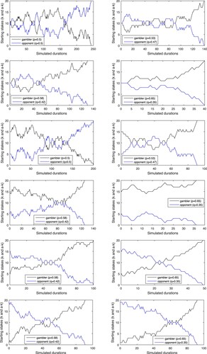
Table 2. The results based on “20, 000” simulations.

p	k	a	${\mu }_k$	$E(T_k)$	$E_k$	$F_k$	$Var(k)$
	1	20	0.2906	43.81	3.31	60.40	885.2094
	5	20	0.0028	49.86	17.54	49.95	246.9837
0.65	10	20	0.0000	33.41	N.O*	33.41	166.3313
	15	20	0.0000	16.53	N.O*	16.53	81.8198
	19	20	0.0000	3.27	N.O*	3.27	15.4067
	1	20	0.5259	53.47	6.20	105.91	3306.4400
	5	20	0.0393	89.15	28.93	91.61	1676.7260
0.58	10	20	0.0017	62.51	59.59	62.51	1180.8172
	15	20	0.0000	31.06	N.O*	31.06	577.7697
	19	20	0.0000	6.38	N.O*	6.38	119.8919
	1	20	0.7821	55.30	15.63	197.70	9513.1150
	5	20	0.2981	152.12	74.31	185.17	13053.9303
0.53	10	20	0.0814	140.84	145.92	140.38	10872.1225
	15	20	0.0201	78.56	188.71	76.30	7229.9460
	19	20	0.0024	15.60	190.17	15.18	1614.5110
	1	20	0.9504	37.70	26.16	258.93	9173.8870
	5	20	0.7452	150.66	117.70	247.06	24868.4300
0.50	10	20	0.4966	200.79	199.75	201.82	26902.3500
	15	20	0.2514	150.43	248.86	117.38	25030.3100
	19	20	0.0513	38.71	271.58	26.12	9289.7061

*Not observed

3.3. Comparative study

In this section, we compare our proposed variant with well-known variations of the gambler ruin's problem in the literature. We consider three most prominent variants of the ruin problem involving: (i) classic framework, (ii) allowing the occurrence of ties and (iii) decision based on successive events. Table 3 documents the comparative performance of contemporary methods with the newly proposed amendment. The comparative performance evaluation is conducted by considering various parametric stetting, which are mentioned in Section 3.1 with $10\mathrm{\%}$ involvements of tie in a single trial. For each method, we calculated the ruin probabilities and expected ruin time corresponding the various influence parameters. The robust performance of the proposed game can be seen throughout the findings in the table. For example, for the case of initial probability 0.65 with initial stake of $1, the classic framework provide the ruin probability as 0.5385 with expected ruin time of 27.43. The game allowing ties reduces the ruin probability by 0.3846 with the increment of one step in game duration. These numbers indicate that the game with ties only favours the stronger player by noticeably reducing his/her ruin probability but on the other hand, it does not offer any advantage to the weaker player by providing minimal extension of the game. Next, the game with successive events, further reduces the ruin probability to 0.2899 and thus favouring the stronger player more openly. On the other hand, we see shocking increase in the game duration from 27 to 88. This un-comprehensible increase in the game duration is due to high likelihood of game resulting in stalemate. On the other hand, one may notice that, the proposed variant offers minimal ruin probability to the stronger player but with sensible increment in game duration. This trend is vividly observable in all consideredparametric settings.

Table 3. Comparison results for classic game (C), involvement of draw (tie) (D), successive trials (S) and proposed game (P).

			${\mu }_k$				$E(T_k)$
p	k	C	D	S	P	C	D	S	P
	1	0.5385	0.3846	0.2899	0.2899	27.43	28.27	88.00	44.00
	5	0.0453	0.0084	0.0020	0.0020	46.98	37.08	99.74	49.87
0.65	10	0.0020	0.0001	0.0000	0.0000	33.20	25.00	66.66	33.33
	15	0.0001	0.0000	0.0000	0.0000	16.66	12.50	33.34	16.67
	19	0.0000	0.0000	0.0000	0.0000	03.33	02.50	06.66	03.33
	1	0.7237	0.5517	0.5244	0.5244	28.29	30.64	106.42	53.21
	5	0.1979	0.0511	0.0396	0.0396	69.02	53.76	177.60	88.80
0.58	10	0.0381	0.0026	0.0016	0.0016	57.73	38.263	124.62	62.31
	15	0.0063	0.0001	0.0001	0.0001	30.46	19.22	62.50	31.25
	19	0.0006	0.0000	0.0000	0.0000	06.18	03.85	12.50	06.25
	1	0.8755	0.6979	0.7846	0.7846	24.82	31.51	110.24	55.12
	5	0.5035	0.1652	0.2950	0.2950	82.17	73.10	303.34	151.67
0.53	10	0.2312	0.0268	0.0830	0.0830	89.59	59.16	278.04	139.02
	15	0.0819	0.0038	0.0192	0.0192	56.04	30.77	153.88	76.94
	19	0.0127	0.0003	0.0022	0.0022	12.43	06.21	31.88	15.92
	1	0.9500	0.7977	0.9500	0.9500	19.00	30.47	76.00	38.00
	5	0.7500	0.3198	0.7500	0.7500	75.00	86.03	300.00	150.00
0.50	10	0.5000	0.0970	0.5000	0.5000	100.00	80.61	400.00	200.00
	15	0.2500	0.0239	0.2500	0.2500	75.00	45.21	300.00	150.00
	19	0.0500	0.0029	0.0500	0.0500	19.00	09.42	76.00	38.00

4. Summary

In this research, we present an extension of the classic 2-player ruin's problem. The proposed variant is based on use of multiple devices simultaneously while deciding a gain or loss. The rationale of the proposition then lies in extended ruin time of the game and thus providing a chance to make a come back to both players. Lengyel [22] extended the game in one direction by allowing ties, i.e. increased the ruin time of the game and this strategy is in the favour of that player who plays with $p>1/2$. The proposed strategy is useful in both directions, i.e. increasing the game duration which is in the favour of that player who plays with $p<1/2$ and decreases the ruin probability for other one who plays with $p>1/2$. The legitimacy of the devised scheme is mathematically established and rigorously verified, numerically and through simulation. In future, it will be interesting to extent the proposed amendment for the more complex formation involving n>2 players.

Acknowledgments

The authors are very grateful to the anonymous editor and referees for providing several constructive and helpful suggestions which led to a significant improvement of the paper.

Disclosure statement

No potential conflict of interest was reported by the author(s).

References

- Edwards A. Pascal's problem – the gambler's ruin'. Int Stat Rev. 1983;51:73–79.
- Morrow GJ. Laws relating runs and steps in gambler's ruin. Stoch Process Their Appl. 2015;125(5):2010–2025.
- Hussain A, Cheema SA, Hanif M. A game based on successive events. Stat. 2020;9(1):e274.
- Perotto FS, Trabelsi I, Combettes S, et al. Deciding when to quit the gambler's ruin game with unknown probabilities. Int J Approx Reason. 2021;137:16–33.
- Hussain A, Cheema SA, Haroon S, et al. The ruin time for 3-player gambler's problem: an approximate formula. Commun Stat Simul Comput. 2021;0:1–9. https://doi.org/10.1080/03610918.2021.1888996.
- Scott J. The probability of bankruptcy: a comparison of empirical predictions and theoretical models. J Bank Financ. 1981;5(3):317–344.
- Snell JL. Gambling, probability and martingales. Math Intell. 1982;4(3):118–124.
- Harik G, Cantu-Paz E, Goldberg DE, et al. The gambler's ruin problem, genetic algorithms, and the sizing of populations. Evol Comput. 1999;7(3):231–253.
- El-Shehawey MA. Absorption probabilities for a random walk between two partially absorbing boundaries: I. J Phys A: Math Gen. 2000;33(49):9005–9013.
- Tsai CW, Hsu Y, Lai K, et al. Application of gambler's ruin model to sediment transport problems. J Hydrol (Amst). 2014;510:197–207.
- Lardizabal CF, Souza RR. Open quantum random walks: ergodicity, hitting times, gambler's ruin and potential theory. J Stat Phys. 2016;164(5):1122–1156.
- Petteruti SF. Fast simulation of random walks on the endoplasmic reticulum by reduction to the gambler's ruin problem [Ph.D. thesis]. Cambridge, MA: Harvard University; 2017.
- Jayasekera R. Prediction of company failure: past, present and promising directions for the future. Int Rev Financ Anal. 2018;55:196–208.
- Feller W. An introduction to probability theory and its applications, vol. I. New York: John Wiley & Sons; 1968.
- Stern F. Conditional expectation of the duration in the classical ruin problem. Math Mag. 2018;48(4):200–203.
- Bach E. Moments in the duration of play. Stat Probab Lett. 1997;36(1):1–7.
- Andel J, Hudecova S. Variance of the game duration in the gambler's ruin problem. Stat Probab Lett. 2012;82(9):1750–1754.
- Kmet A, Petkovsek M. Gambler's ruin problem in several dimensions. Adv Appl Math. 2002;28(2):107–118.
- Ethier SN. Gambler's ruin. In: The doctrine of chances, probability and its applications. Berlin: Springer; 2010. p. 241–274.
- Lefebvre M. The gambler's ruin problem for a Markov chain related to the Bessel process. Stat Probab Lett. 2008;78(15):2314–2320.
- El-Shehawey MA. On the gambler's ruin problem for a finite Markov chain. Stat Probab Lett. 2009;79(14):1590–1595.
- Lengyel T. The conditional gambler's ruin problem with ties allowed. Appl Math Lett. 2009;22(3):351–355.
- Harper JD, Ross KA. Stopping strategies and gambler's ruin. Math Mag. 2018;78(4):255–268.
- Lorek P. Generalized gambler's ruin problem: explicit formulas via siegmund duality. Methodol Comput Appl Probab. 2017;19(2):603–613.
- Hussain A, Cheema SA. The classic two-player gambler's ruin problem with successive events: a generalized variance. Comput Math Methods. 2021;3:e1156.
- Samuels SM. The classical ruin problem with equal initial fortunes. Math Mag. 2018;48(5):286–288.