
 ?Mathematical formulae have been encoded as MathML and are displayed in this HTML version using MathJax in order to improve their display. Uncheck the box to turn MathJax off. This feature requires Javascript. Click on a formula to zoom.
Abstract
In this paper, a modified Korteweg–de Vries equation with a quartic nonlinear term in two-electron temperature plasmas is studied. Firstly, the symmetries are constructed using the generalized symmetry method. In addition, the potential equation is studied, it can been found that this equation does not posses potential symmetries. Meanwhile, the symmetry reduction and group-invariant solutions are derived rely on the one-dimensional optimal system of subalgebras. Finally, conservation laws are showed resort by the multipliers method, three polynomial type conserved quantities are presented, also the Hamiltonian form is obtained. In particular, reciprocal Bäcklund transformations for conservation laws are obtained for the first time.
1. Introduction
In the present paper, we focus on the following equation [Citation1]:
(1)
(1) which is derived from the following equations:
(2)
(2) In paper [Citation1], the authors derived this equation, and give solutions and three conservation laws. Motivated by their works, we will study this model from view of symmetry. Because this equation is derived from the actual physical background, it is necessary for us to study it. For this equation, we have not found any author to deal with them in the symmetry method. In fact, this equation belongs to one of the Korteweg de Vries (KdV) family of equations, many authors use various methods to deal with KdV family of equations. We known that the KdV equation is a famous equation in mathematics and physics, which was initially proposed by Korteweg and de Vries [Citation2], this equation was mainly established for surface waves on shallow water. And then, many scientists found that this equation has important applications in many fields [Citation3–6]. In that paper [Citation6], they derived a KdV type equation and obtained some soliton solutions. In our paper, we mainly focus on symmetry and conservation laws for Equation (Equation1
(1)
(1) ). Many papers have studied high-order KdV equation [Citation7, Citation8] (and the references therein).
We know that nonlinear science is an important modern science and plays an important role in many fields. Nonlinear evolution equations can be used to describe many complex natural phenomena [Citation9–12]. A natural problem naturally arises: How to solve these nonlinear evolution equation? On the one hand, these equations reflect some natural phenomena and provide a basis for many practical problems; on the other hand, many authors are trying to find some methods to solve the nonlinear evolution equations. We know that until now, there is no unified method to solve nonlinear evolution equations. However, fortunately, after the continuous efforts of many authors, some methods for solving nonlinear evolution equations have been proposed and developed. Some important methods include Lie group methods [Citation13–26], Douboux transformation, Lax pairs, inverse scattering transformation, nonlocal symmetry and so on.
Although this model is simple, it is still necessary to study this equation from another perspective. Firstly, we investigate this equation from view of the symmetry method, and then, symmetry reductions and explicit solutions are given. Meanwhile, conservation laws also derived using the multipliers method, it should be emphasized that we obtain the reciprocal Bäcklund transformations for conservation laws of this equation for the first time.
2. Symmetries analysis for Equation (1)
2.1. Generalized symmetries for Equation (1)
From the generalized symmetry method [Citation14] (pp. 248–250) and [Citation15], for a given nonlinear evolution equation
(3)
(3) that is to say, for a function σ, it is a symmetry of Equation (Equation3
(3)
(3) ), when it satisfies
(4)
(4) for all solutions u, where
(5)
(5) Hence, we get
(6)
(6) Now, setting σ,
(7)
(7) where a, b, e, g are functions of t, x to be determined. Replacing (Equation7
(7)
(7) ) into (Equation6
(6)
(6) ) and employing (Equation1
(1)
(1) ), replacing
by
, In this way, one should get some partial differential equations, solve them by hand, and obtain
(8)
(8) here
are arbitrary constants. Putting (Equation8
(8)
(8) ) into (Equation7
(7)
(7) ), we have
(9)
(9) It is equivalent to
(10)
(10) In this way, one can get the vector field
(11)
(11) or
(12)
(12)
2.2. Potential symmetry analysis
For the conservation laws forms,
(13)
(13) where T is the conserved density and X is the conserved flow, we rewrite Equation (Equation1
(1)
(1) ), the following should be obtained
(14)
(14) From the Lie symmetry analysis method [Citation13] (Chapter 2) [Citation16] (Chapter 1), one can obtain the coefficient functions
,
,
and
as
(15)
(15) where
) are arbitrary constants.
It is shown that this equation does not posses potential symmetries. Consequently, we also derive the potential equation
(16)
(16) Like the previous steps, we can get the following results for the potential equation:
(17)
(17) Therefore, we can get the vector fields for potential equation (Equation16
(16)
(16) )
(18)
(18)
3. Similarity reduction and exact solutions of Equation (1)
3.1. One-dimensional optimal system
Using the adjoint transformations formula [Citation13]
(19)
(19) where ϵ is a nonzero constant.
is the commutator for the Lie algebra
(20)
(20) One can derive an optimal system as
(21)
(21)
3.2. Symmetry reductions
In this subsection, we employ the optimal system of one-dimensional subalgebras to deal with (Equation1(1)
(1) ).
For this case
, trivial solution
Consider the generator , one can derive the group-invariant solution
(22)
(22) where
. Inserting (Equation22
(22)
(22) ) into (Equation1
(1)
(1) ), following ODE is given
(23)
(23) Integrating, we have
(24)
(24) where k is an integration constant. If we assume k = 0, and multiplied by
, and integral once, one can get
(25)
(25)
| (3) | |||||
For the vector , one can get
(26)
(26) Substitution of (Equation26
(26)
(26) ) into (Equation1
(1)
(1) ), we get
(27)
(27)
4. Explicit solutions of Equation (1) via Equation (27)
Supposing that (Equation27(27)
(27) ) has the following solution:
(28)
(28) Putting (Equation28
(28)
(28) ) into (Equation27
(27)
(27) ), which leads to
(29)
(29) Let n = 0 in (Equation29
(29)
(29) ), one has
(30)
(30) For the more general case of
, it generates
(31)
(31) Thus, the power series solution is given by
(32)
(32) In other words, at last we get a solution of (Equation1
(1)
(1) )
(33)
(33) here
are arbitrary constants. Generally speaking, the series solution is convergent. If we consider n = 3, we get approximate solution as the following form:
(34)
(34) here
are arbitrary constants.
5. Exact travelling wave solution of Equation (1)
Now we study Equation (Equation1(1)
(1) ) has the following hypothetical solution [Citation6, Citation27, Citation28]:
(35)
(35) where
,
are constants need to be fixed. On the basis of Equation (Equation35
(35)
(35) ), it generates
(36)
(36) Putting Equation (Equation36
(36)
(36) ) into Equation (Equation1
(1)
(1) ), one has
(37)
(37) Considering the exponents
and p + 2 should be equal, one finds
(38)
(38) also, one gets
(39)
(39) therefore, one can get
(40)
(40) For the coefficient of term
, one can yield
(41)
(41) Finally, we get the soliton solution as
(42)
(42) In fact, this solution is equivalent to the solution in reference [Citation1], which we derive from a different perspective.
Also considering Equation (Equation1(1)
(1) ) has the following hypothetical solution:
(43)
(43) where
,
are constants need to be calculated. On the basis of Equation (Equation43
(43)
(43) ), it generates
(44)
(44) Putting Equation (Equation44
(44)
(44) ) into Equation (Equation1
(1)
(1) ), one gets
(45)
(45) Using the same method, one can obtain
(46)
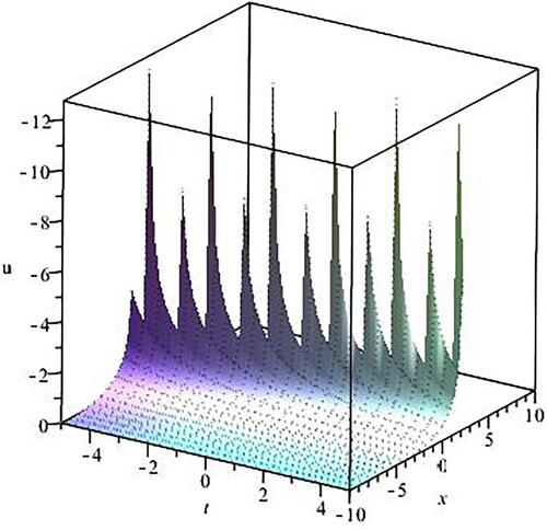
(46) At last, a soliton solution is given by
(47)
(47) Some special cases of the solution (B = 1) are shown in Figures and .
Figure 1.
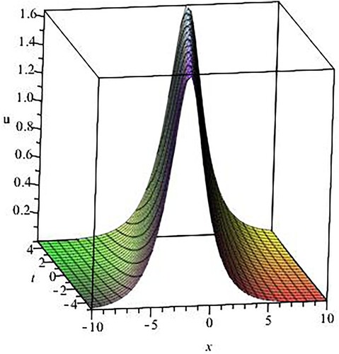
Figure 2.
6. Conservation laws
In this section, by employing the multipliers method [Citation16], one can get the multipliers,
(48)
(48) For the case multiplier
, we have,
(49)
(49) One can assume that this conservation law means conservation of energy.
For the multiplier u, we get
(50)
(50) This conservation laws can been seen as conservation of momentum.
Consider the multiplier 1, one has
(51)
(51) This conservation laws presents the conservation of mass.
In this way, one can get the three polynomial type conserved quantities
(52)
(52) Therefore, we can rewrite (Equation1
(1)
(1) ) in the following Hamiltonian form:
(53)
(53)
6.1. Conservation laws of potential equation (16)
For the potential equation, one obtains the fourth-order multipliers,
(54)
(54) For the multiplier
, one can get
(55)
(55) Consider the multiplier
, one should derive
(56)
(56)
7. Reciprocal Bäcklund transformations of conservation laws
In paper [Citation29], the authors derived the reciprocal Bäcklund transformations of conservation laws. On the basis of that paper, one has
Theorem 7.1
[Citation29]
The conservation law
(57)
(57) is connected reciprocally to associated conservation law
(58)
(58) using the reciprocal transformation
(59)
(59) where
(60)
(60)
Therefore, as to multiplier , we get reciprocal Bäcklund transformations of conservation laws for (Equation49
(49)
(49) ),
(61)
(61) If the multiplier is u, we get
(62)
(62) If the case multiplier is 1, we have
(63)
(63) or equivalently
(64)
(64) Using the same steps, we can derive reciprocal Bäcklund transformations for conservation laws of the potential equation.
For the multiplier , one can get reciprocal Bäcklund transformations
(65)
(65) When the multiplier is
, one can arrive at
(66)
(66)
8. Conclusions
In the present paper, we investigated the symmetries, symmetry reductions and conservation laws of a modified Korteweg–de Vries equation with a quartic nonlinear term. First, we employed a generalized symmetry analysis method to derive symmetries for this equation, and get its infinitesimal generators. Also, some explicit solutions and conservation laws are presented. Meanwhile, reciprocal Bäcklund transformations for conservation laws are showed for the first time.
In this paper, we studied this equation based on the symmetry method, and we presented the potential symmetry of this equation, and we found that this equation, for our hypothesis, does not have potential symmetry. Using Lie algebra, we derived an optimal system for this equation, and using the optimal system, we have simplified this equation. Then the series method is used to obtain the explicit solution of the original equation. Then the reciprocal Bäcklund transformations for conservation laws of the equation are obtained. The conservation law of the potential equation and the reciprocal Bäcklund transformations for conservation laws of the potential equation are also studied. We found that the symmetry group method is a very effective method to deal with differential equations.
These results are of great help to explain the complicated nonlinear physical phenomena. In this paper, we studied a simple cubic nonlinear equation model, where there are still many issues to be considered, such as discrete case, fractional order case, variable coefficient case and so on. These topics will be reported in future works.
Disclosure statement
No potential conflict of interest was reported by the author(s).
References
- Verheest F, Olivier CP, Hereman WA. Modified Korteweg-de Vries solitons at supercritical densities in two-electron temperature plasmas. J Plas Phys. 2016;82(2):905820208.
- Korteweg DJ, de Vries G. On the change of form of long waves advancing in a rectangular canal, and on a new type of long stationary waves. Philos Mag. 1895;39:422–443.
- Zabusky NJ, Kruskal MD. Interaction of solitons in a collisionless plasma and the recurrence of initial states. Phys Rev Lett. 1965;15:240–243.
- Washimi H, Taniuti T. Propagation of ion-acoustic solitary waves of small amplitude. Phys Rev Lett. 1966;17:996–998.
- Miura RM, Gardner CS, Kruskal MD. Korteweg-de Vries equation and generalizations. II. Existence of conservation laws and constants of motion. J Math Phys. 1968;9:1204–1209.
- El-Tantawy SA, Wazwaz AM. Anatomy of modified Korteweg-de Vries equation for studying the modulated envelope structures in non-Maxwellian dusty plasmas: freak waves and dark soliton collisions. Phys Plas. 2018;25:092105.
- Wazwaz A-M. The tanh and the sine-cosine methods for the complex modified KdV and the generalized K dV equations. Comput Math Appl. 2005;49:1101–1112.
- Wang GW, Liu Y, Wu Y. Symmetry analysis for a seventh-order generalized KdV equation and its fractional version in fluid mechanics. Fractals. 2020;28:2050044.
- El-Tantawy SA, Salas AH, Alharthi MR. Novel analytical cnoidal and solitary wave solutions of the extended Kawahara equation. Chaos Solitons Fract. 2021;147:110965.
- El-Tantawy SA, Salas AH, Alharthi MR. On the dissipative extended Kawahara solitons and cnoidal waves in a collisional plasma: novel analytical and numerical solutions. Phys Fluids. 2021;33:106101.
- Kashkari BS, El-Tantawy SA. Homotopy perturbation method for modeling electrostatic structures in collisional plasmas. Eur Phys J Plus. 2021;136:121.
- El-Tantawy SA. Nonlinear dynamics of soliton collisions in electronegative plasmas: the phase shifts of the planar KdV- and mkdV-soliton collisions. Chaos Solitons Fract. 2016;93:162–168.
- Olver PJ. Application of Lie group to differential equation. New York: Springer; 1986.
- Tian C. Lie groups and its applications to differential equations. Beijing: Science Press; 2001(in Chinese).
- Wang GW, Liu XQ, Ying YY. Symmetry reduction, exact solutions and conservation laws of a new fifth-order nonlinear integrable equation. Commun Nonlinear Sci Numer Simulat. 2013;18:2313–2320.
- Bluman GW, Cheviakov AF, Anco SC. Applications of symmetry methods to partial differential equations. New York: Springer; 2010.
- Wang GW, Kara AH, Fakhar K. Symmetry analysis and conservation laws for the class of time-fractional nonlinear dispersive equation. Nonlinear Dyn. 2015;82:281–287.
- Wang GW, Liu XQ, Ying YY. Lie symmetry analysis to the time fractional generalized fifth-order KdV equation. Commun Nonlinear Sci Numer Simulat. 2013;18:2321–2326.
- Wang GW, Yang K, Gu H, et al. A (2+1)-dimensional sine-Gordon and sinh-Gordon equations with symmetries and kink wave solutions. Nucl Phys B. 2020;953:114956.
- Wang GW, Vega-Guzman J, Biswas A, et al. (2+1)-dimensional Boiti-Leon-Pempinelli equation-Domain walls, invariance properties and conservation laws. Phys Lett A. 2020;384:126255.
- Wang GW, Kara AH. A (2+1)-dimensional KdV equation and mKdV equation: symmetries, group invariant solutions and conservation laws. Phys Lett A. 2019;383:728–731.
- Wang GW, Kara AH. Group analysis, fractional explicit solutions and conservation laws of time fractional generalized Burgers equation. Commu Theor Phys. 2018;69(1):5–8.
- Wang GW. Symmetry analysis and rogue wave solutions for the (2+1)-dimensional nonlinear Schrodinger equation with variable coefficients. Appl Math Lett. 2016;56:56–64.
- Wang GW. A new (3+1)-dimensional Schrodinger equation: derivation, soliton solutions and conservation laws. Nonlinear Dyn. 2021;104:1595–1602.
- Wang GW. A novel (3+1)-dimensional sine-Gorden and a sinh-Gorden equation: derivation, symmetries and conservation laws. Appl Math Lett. 2021;113:106768.
- Wang GW. Symmetry analysis, analytical solutions and conservation laws of a generalized KdV-Burgers-Kuramoto equation and its fractional version. Fractals. 2021;29:2150101.
- Triki H, Hayat T, Aldossary OM. Solitary wave and shock wave solutions to a second order wave equation of Korteweg-de Vries type. Appl Math Comp. 2011;217:8852–8855.
- Wang GW, Wazwaz AM. On the modified Gardner type equation and its time fractional form. Chaos Solitons Fract. 2022;155:111694.
- Kingston JG, Rogers C. Reciprocal Bäcklund transformations of conservation laws. Phys Lett A. 1982;92:261–264.