Consistent travelling waves solutions to the non-linear time fractional Klein–Gordon and Sine-Gordon equations through extended tanh-function approach

Abstract

In this study, the extended tanh-function method has been used to find further general travelling wave solutions for space-time fractional nonlinear partial differential equations, namely, the time fractional nonlinear Sine-Gordon equation and Klein–Gordon equation. The mentioned equations are useful for explaining a series of experimental seismic data, modelling of strain waves, and structures correlated to fault dynamics and the subduction slab, as well as slow earthquakes, episodic tremor, slow slip events, and tremor migration patterns. This method is used to attain exact solutions to a variety of nonlinear partial differential equations that were spatially temporal fractional. To get analytical solutions of the travelling wave type of certain nonlinear evolution equations, a power series in tanh was first utilized as an ansatz. These nonlinear fractional partial differential equations (NLFPDEs) are solved on a variety of non-rectangular domains. By using the fractional complex transform and the properties of the confirmable derivative, the two equations are reduced to ordinary differential equations. The solutions are sketched in 3D, and contour patterns, including king type, single soliton, double solitons, multiple solitons, bell shape, and other sorts of solutions. The achieved solutions are very much effective for explaining the above-stated phenomena.

KEYWORDS:

• The time fractional Kelin–Gordon equation
• the time fractional Sine-Gordon equation
• conformable derivative
• travelling wave solution
• the extended tanh-function method

MSC::

• 35C25
• 35C07
• 35C08
• 35Q20
• 76B25

1. Introduction

Nonlinear fractional partial differential equations (NLFPDEs) are commonly used to formulate real-world problems from a mathematical perspective. There are a variety of instances in which simulations of such situations are essential. A huge amount of literature by numerous authors from diverse fields of study has recently been presented that deals with dynamical systems, mathematical physics, and engineering defined by fractional differential equations. Ordinary differential equations are generalized to arbitrary (non-integer) order by fractional differential equations. Power law memory kernels capture nonlocal spatial and temporal interactions in fractional differential equations. Because fractional differential equations are used in so many fields of engineering and science, scientific research into them has proliferated. Many scholars [1–4] have looked at fractional differential equations and used various solutions approaches. Fractional derivatives and integrals were once regarded to be the domain of theoretical mathematics. However, many investigations in the preceding few decades have suggested that fractional phenomenon is linked not only in mathematics but also in applied mathematics and engineering disciplines such as vascular mechanics, fluid mechanics, optical fibres, geochemistry, solid-state physics, control theory, water waves mechanics, plasma physics, and to such a great extent. The advantage of fractional derivatives in modelling mechanical and electrical properties of real materials becomes apparent due to the ignoring of effects in standard integer-order models. Fractional derivatives serve as a foundation for describing the characteristics of mathematics. Numerous excellent strategies for solving these systems have been discovered in recent years in the most useful research on NLFPDEs, for example, the exp-function approach [5–8], the Kudryashov method [9,10], and the complex transform approach [11,12]. Many fundamental occurrences in non-Brownian motion, signal processing, control difficulties, viscoelastic materials, polymers, systems identification, and other branches of science and engineering are well represented by NLFPDEs [13]. There have been numerous powerful approaches for obtaining numerical and analytical solutions to NLFPDEs developed and established, the bifurcation method [14], finite element method [15], the tan $(\phi /2)$ method [16,17], differential transform method [18], the multiple Rogue-wave solution method [19], the auxiliary equation method [20], the Jacobi elliptic function method [21], homotopy perturbation method [22], the extended rational sine cosine method [23], the double $(G^{\mathrm{\prime }}/G,1/G)$-expansion method [24], the extended tanh-function method [25,26], the group preserving scheme [27], and semi-inverse variational method [28]. The question of how to expand existing approaches to tackle other NLFPDEs remains an intriguing and significant research topic. Thanks to the efforts of various researchers, several NLFPDEs have been examined and solved, including the impulsive fractional differential equations [29], space-time fractional advection–dispersion equation [30–32], fractional generalized Burgers’ fluid [33], and fractional heat and mass-transport equation [34], etc.

The Klein–Gordon equation correctly explains the spinless pion and de Broglie waves and thus plays an important role in mathematical physics and numerous scientific applications, including solid-state physics, nonlinear optics, and quantum field theory. The equation has become a lot of interest in the field of solitons and condensed matter physics, as well as in the study of solitons in a collisionless plasma, the recurrence of starting states, and nonlinear wave equations. This equation is used in a mathematical model in a variety of scientific fields, including solid-state physics, nonlinear optics, and quantum field theory. Golmankhaneh et al. [35] used the homotopy perturbation approach to investigate the nonlinear fractional Klein–Gordon equation. The first integral technique for some time fractional differential equations, fractional Klein–Gordon equation, fractional Hirota–Satsuma coupled KdV system as well as fractional Sharma–Tasso–Olever equation was introduced by Lu [36]. The analytical approximate solution of the nonlinear space-time fractional Klein–Gordon equation was recently obtained by Gepreel and Mohamed [37]. Put on the homotopy analysis method, Jafari et al. [38] applied the fractional sub-equation method to explore the Cahn–Hilliard and the Klein–Gordon equations. Furthermore, Ran and Zhang [39] adopted the compact difference approach for the space fractional Klein–Gordon equation. Riccati expansion [40–42], modified extended Tanh [43], the $(G^{\mathrm{\prime }}/G)$ and $(w/g)\text{ - }$ expansion [44] methods are also applied to search for the exact solutions of the space-time fractional Klein–Gordon equation.

The space-time fractional Sine-Gordon equation is a sine function used in domains such as wave propagation, classical lattice dynamics, biological membrane extension, crystal defect spread, relativistic field theory, and others. The fractional Sine-Gordon equation is also useful for explaining a series of experimental seismic data, modelling of strain waves, and structures correlated to fault dynamics and the subduction slab, as well as slow earthquakes, episodic tremor, slow slip (ETS) events, and tremor migration patterns. Zhou et al. [45] studied the soliton solutions to the coupled Sine-Gordon problem in nonlinear optics using the Jacobi elliptic function approach. Hosseini et al. [46] recently discovered fresh accurate solutions to the linked Sine-Gordon equation.

The extended tanh-function method has not yet been used to explore the space-time fractional Klein–Gordon equation and space-time fractional Sine-Gordon equation. As a consequence, the objective of this work is to use the extended tanh-function method to find novel results for the above-mentioned equations. The advantages of this method over other ways are that it allows us to obtain more arbitrary constants and different sorts of solutions. Aside from the basic application, it also aids numerical solvers in assessing the validity of their conclusions and assisting them in instability analysis.

The article’s layout is ordered as follows: In Section 2, we go over several definitions and features of the Confirmable derivative. We show how to discover accurate travelling wave solutions to NLFPDEs in Section 3. In Section 4, we look at a new closed-form wave solution for the general space-time fractional Klein–Gordon equation and space-time fractional Sine-Gordon equation. In Section 5, the findings and debates are evaluated using graphical representations and physical clarifications. In Section 6, the comparison between our achieved solution and other existing literature are presented, and lastly, conclusions are formed in Section 7.

2. Meaning and foreword

The conformable derivative is simpler and more efficient, which reflects a natural extention of the normal derivative to solve fractional-order nonlinear partial differential equations. Moreover, it does not have any delay effect, like the other fractional ones (Caputo derivative, Reimann–Livoulli derivative) have. Let us consider, $f:[0,\mathrm{\infty })\to \mathbb{R}$, is a function. The $\alpha$-order “conformable derivative” of $f$ is defined as [47]: (1) $P_{\alpha }(f)(t)=\underset{\epsilon \to 0}{lim}\frac{f(t+\epsilon t^{1-\alpha })-f(t)}{\epsilon },$(1) for every $t>0,\alpha \in (0,1)$. If $f$ be $\alpha$-differentiable in some $(0,a)$, $a>0$ and $\underset{t\to 0^{+}}{lim}{f}^{(\alpha )}(t)$ exists, then define $f^{(\alpha )}(0)=\underset{t\to 0^{+}}{lim}{f}^{(\alpha )}(t)$. The theorems that follow highlight a few axioms that are fulfilled conformable derivatives.

Theorem 2.1:

Assume $\alpha \in (0,1]$ and also supposed $f,g$ be $\alpha$-differentiable at a point $t>0$. Hence

• $P_{\alpha }(xf+yg)=x{P}_{\alpha }(f)+y{P}_{\alpha }(g),forallx,y\in \mathbb{R}.$

• $P_{\alpha }(t^z)=q{t}^{p-\alpha },forallz\in \mathbb{R}.$

• $P_{\alpha }(u)=0,forallconstantfunctionf(t)=u.$

• $P_{\alpha }(fg)=f{P}_{\alpha }(g)+g{P}_{\alpha }(f).$

• $P_{\alpha }\left(\frac{f}{g}\right)=\frac{g{P}_{\alpha }(f)-f{P}_{\alpha }(g)}{g^2}.$

• $Inaddition,iffisdifferentiable,thenP{T}_{\alpha }(f)(t)=t^{1-\alpha }\frac{df}{dt}.$

Khalil et al. [47] consider various more properties, such as the chain law, Gronwall’s inequality, integration methods, the Laplace transform, Tailor series expansion, and the exponential function in terms of conformable derivative.

Theorem 2.2:

Assume $f$ is an $\alpha$-differentiable function in conformable differentiable and suppose that $g$ is also differentiable and defined in the range of $f$. Now (2) $M_{\alpha }(f\circ g)(t)=t^{1-\alpha }{g}^{\mathrm{\prime }}(t)f_g(t).$(2)

3. Essential facts and the enactment of the procedures

At this stage, the extended tanh-function approach is defined for obtaining numerous exact solutions for fractional nonlinear evolution equations (FNLEEs), as detailed by Wazwaz [48]. The main concept underlying the proposed method is to characterize the solution as a polynomial in hyperbolic functions, and then solve the variable coefficient PDE using a first-order ODE and algebraic eigenvalues approach. To start with, we apprehend an FNLEE associated with a function $U=U(x,t)$ as follows: (3) $\begin{array}{rl}& R(u,D_t^{\alpha }u,D_x^{\beta }u,D_t^{\alpha }{D}_t^{\alpha }u,D_t^{\alpha }{D}_x^{\beta }u,D_x^{\beta }{D}_x^{\beta },\dots \dots \dots )\\ & =0,0<\alpha \le 1,0<\beta \le 1,\end{array}$(3) where $u$ is an unidentified function with spatial and temporal derivatives $x$ and $t$, $\alpha$ and $\beta$ are fractional-order derivatives, and $P$ is a polynomial of $u(x,t)$ and its derivatives in which the maximal order of derivatives and nonlinear terms of the maximal order are related. Consider how waves change over time. (4) $\xi =k\frac{x^{\beta }}{\beta }+c\frac{t^{\alpha }}{\alpha },u(x,t)=u(\xi ),$(4) here $c$ as well as $k$ are random nonzero constants.

It is rewritten as follows after applying the wave transformation in (3): (5) $R(u,u^{\mathrm{\prime }},u^{\mathrm{\prime }\mathrm{\prime }},u^{\mathrm{\prime }\mathrm{\prime }\mathrm{\prime }},\dots \dots \dots )=0,$(5) where the ordinary derivative of $u$ is denoted by the superscripts.

Phase 3.1: Let us consider a formal solution of ODE in the following structure (6) $u(\xi )=\sum _{i=0}^n{a}_i{Y}^i+\sum _{i=1}^n{b}_i{Y}^{-i},$(6) for which (7) $Y=\text{tanh}(\mu \xi ),$(7) where $\mu$ can be some arbitrary value.

Phase 3.2: Define the positive constant $\eta$ by finding the homogeneous equilibrium between the maximum order nonlinear terms and their derivatives in Equation (5).

Phase 3.3: By replacing solution (6) and (7) with Equation (5) with the value of $\eta$ attained in Phase 3.2, polynomials in $Y$ are obtained. Set all of the coefficients of the resulting polynomials to zero produces a set of algebraic equations $a_i^{\mathrm{\prime }}s$ along with $b_i^{\mathrm{\prime }}s$. Solve these equations $a_i^{\mathrm{\prime }}s$ along with $b_i^{\mathrm{\prime }}s$ using symbolic computation tools like Maple.

Phase 3.4: We create closed-form moving wave solutions of the nonlinear evolution Equation (6) by inserting values from Phase 3.3 into Equation (6) along with Equation (7) and (3).

4. Analysis of the solutions

In this section, we create some novel and more general closed-form travelling wave solutions to the time fractional Kelin–Gordon and Sine-Gordon equations by means of the extended tanh-function technique.

4.1. The nonlinear fractional Klein–Gordon equation

In this sub-section, we assess exact solutions to the nonlinear fractional Klein–Gordon equation via the innovative extended tanh-function method. Contemplate the fractional Klein–Gordon equation [49] (8) $D_{tt}^{2\alpha }u(x,t)+D_{xx}^{2\alpha }u(x,t)+pu(x,t)-q{u}^2(x,t)=0,$(8) where $p$ and $q$ are nonzero constants, and $\alpha$ is a fractional-order derivative. Taking the travelling wave transformation (9) $\xi =l\frac{x^{\alpha }}{\alpha }-k\frac{t^{\alpha }}{\alpha },u(x,t)=u(\xi ),$(9) here $k$ and $l$ stands for nonzero constants. Equation (8) converts to the following ordinary equation: (10) $(k^2-l^2)U^{\mathrm{\prime }\mathrm{\prime }}+pU-q{U}^2=0.$(10)

By balancing the highest order derivative term with the highest power nonlinear term, balancing number is found to be 2. This procedure provides the especial type of solutions namely solitons. It is a wave or disturbance that is propagated as a travelling non-dissipative wave which is neither preceded nor followed by another such disturbance. From Equation (6), we achieved such soliton-type wave solutions. (11) $u(\xi )=a_0+a_{1}Y+a_2{Y}^2+b_1{Y}^{-1}+b_2{Y}^{-2}.$(11)

Take the place of (10) into (11) along with (7), in $Y$, the left side transforms into a polynomial. When each of the polynomial’s coefficients is set to zero, a set of algebraic equations emerges (destined used for plainness, we omission over them to the exhibition) for $a_0$, $a_1$, $a_2,b_1,b_2,k$ and $l$. The resulting outcomes are gained by applying computer algebra, such as Maple, to resolve this over-determined series of equations:

Cluster 4.1: $\begin{array}{rl}& k=\frac{1}{2}\frac{\sqrt{p+4l^2{\mu }^2}}{\mu },l=l,a_0=-\frac{1}{2}\frac{p}{q},\\ & a_1=0,a_2=0,\text{and}{b}_1=0,b_2=\frac{3}{2}\frac{p}{q}.\end{array}$

In terms of $\text{cot}\text{h}$ functions, the values of the parameters presented in Cluster 4.1 form an explicit solution. (12) $\begin{array}{rl}{u}_1(x,t)& =-\frac{1}{2}\frac{p}{q}+\frac{3}{2}\frac{p}{q}\text{cot}{\text{h}}^2\\ & \times \left(\mu \left(l\frac{x^{\alpha }}{\alpha }-\frac{1}{2}\frac{\sqrt{p+4l^2{\mu }^2}}{\mu }\frac{t^{\alpha }}{\alpha }\right)\right).\end{array}$(12)

Cluster 4.1 is gained from those values of the parameters which construct an explicit result in terms of $\text{cosec}\text{h}$ function. (13) $\begin{array}{rl}{u}_2(x,t)& =-\frac{1}{2}\frac{p}{q}+\frac{3}{2}\frac{p}{q}+\frac{3}{2}\frac{p}{q}\text{cosec}{\text{h}}^2\\ & \times \left(\mu \left(l\frac{x^{\alpha }}{\alpha }-\frac{1}{2}\frac{\sqrt{p+4l^2{\mu }^2}}{\mu }\frac{t^{\alpha }}{\alpha }\right)\right).\end{array}$(13)

Cluster 4.2: $\begin{array}{rl}k& =\frac{1}{2}\frac{\sqrt{p+4l^2{\mu }^2}}{\mu },l=l,a_0=-\frac{1}{2}\frac{p}{q},a_1=0,\\ a_2& =\frac{3}{2}\frac{p}{q}\text{and}{b}_1=0,b_2=0.\end{array}$

The values of the parameters presented in Cluster 4.2 formulate an explicit solution in terms of $\text{tan}\text{h}$ functions. (14) $\begin{array}{rl}{u}_3(x,t)& =-\frac{1}{2}\frac{p}{q}+\frac{3}{2}\frac{p}{q}\text{tan}{\text{h}}^2\\ & \times \left(\mu \left(l\frac{x^{\alpha }}{\alpha }-\frac{1}{2}\frac{\sqrt{p+4l^2{\mu }^2}}{\mu }\frac{t^{\alpha }}{\alpha }\right)\right).\end{array}$(14)

Which can be renovated by Cluster 4.2 dint of the hyperbolic formula and space, time coordinates (15) $\begin{array}{rl}{u}_4(x,t)& =-\frac{1}{2}\frac{p}{q}+\frac{3}{2}\frac{p}{q}\\ & -\frac{3}{2}\frac{p}{q}\text{sec}{\text{h}}^2\left(\mu \left(l\frac{x^{\alpha }}{\alpha }-\frac{1}{2}\frac{\sqrt{p+4l^2{\mu }^2}}{\mu }\frac{t^{\alpha }}{\alpha }\right)\right).\end{array}$(15)

Cluster 4.3: $\begin{array}{rl}k& =\frac{1}{2}\frac{\sqrt{-p+4l^2{\mu }^2}}{\mu },l=l,a_0=\frac{3}{2}\frac{p}{q},a_1=0,\\ a_2& =0\text{and}{b}_1=0,b_2=-\frac{3}{2}\frac{p}{q}.\end{array}$

In terms of $\text{tan}\text{h}$ function the values of the parameters presented in Cluster 4.3 formulate an explicit solution. (16) $\begin{array}{rl}{u}_5(x,t)& =\frac{3}{2}\frac{p}{q}-\frac{3}{2}\frac{p}{q}\text{cot}{\text{h}}^2\\ & \times \left(\mu \left(l\frac{x^{\alpha }}{\alpha }-\frac{1}{2}\frac{\sqrt{-p+4l^2{\mu }^2}}{\mu }\frac{t^{\alpha }}{\alpha }\right)\right).\end{array}$(16)

Which can be renovated by dint of the hyperbolic formula and space, time coordinates (17) $\begin{array}{rl}{u}_6(x,t)& =\frac{3}{2}-\frac{3}{2}\frac{p}{q}-\frac{3}{2}\frac{p}{q}\text{cosec}{\text{h}}^2\\ & \times \left(\mu \left(l\frac{x^{\alpha }}{\alpha }-\frac{1}{2}\frac{\sqrt{-p+4l^2{\mu }^2}}{\mu }\frac{t^{\alpha }}{\alpha }\right)\right).\end{array}$(17)

Cluster 4.4: $\begin{array}{rl}k& =\frac{1}{4}\frac{\sqrt{p+16l^2{\mu }^2}}{\mu },l=l,a_0=\frac{1}{4}\frac{p}{q},a_1=0,\\ a_2& =\frac{3}{8}\frac{p}{q}\text{and}{b}_1=\frac{1}{2},b_2=\frac{3}{8}\frac{p}{q}.\end{array}$

The values of the parameters presented in Cluster 4.4 formulate an explicit solution in terms of $\text{tan}\text{h}$ and $\text{cot}\text{h}$ function. (18) $\begin{array}{rl}{u}_7(x,t)& =\frac{1}{4}\frac{p}{q}+\frac{3}{8}\frac{p}{q}\text{tan}{\text{h}}^2\\ & \times \left(\mu \left(l\frac{x^{\alpha }}{\alpha }-\frac{1}{4}\frac{\sqrt{p+16l^2{\mu }^2}}{\mu }\frac{t^{\alpha }}{\alpha }\right)\right)\\ & +\frac{3}{8}\frac{p}{q}\text{cot}{\text{h}}^2\\ & \times \left(\mu \left(l\frac{x^{\alpha }}{\alpha }-\frac{1}{4}\frac{\sqrt{p+16l^2{\mu }^2}}{\mu }\frac{t^{\alpha }}{\alpha }\right)\right).\end{array}$(18)

The hyperbolic formula and space, time coordinates can be used to reconstruct it. (19) $\begin{array}{rl}{u}_8(x,t)& =\frac{1}{4}\frac{p}{q}+\frac{3}{8}\frac{p}{q}-\frac{3}{8}\frac{p}{q}\text{sec}{\text{h}}^2\\ & \times \left(\mu \left(l\frac{x^{\alpha }}{\alpha }-\frac{1}{4}\frac{\sqrt{p+16l^2{\mu }^2}}{\mu }\frac{t^{\alpha }}{\alpha }\right)\right)\\ & +\frac{3}{8}\frac{p}{q}\text{cot}{\text{h}}^2\\ & \times \left(\mu \left(l\frac{x^{\alpha }}{\alpha }-\frac{1}{4}\frac{\sqrt{p+16l^2{\mu }^2}}{\mu }\frac{t^{\alpha }}{\alpha }\right)\right).\end{array}$(19)

And (20) $\begin{array}{rl}{u}_9(x,t)& =\frac{1}{4}\frac{p}{q}+\frac{3}{8}\frac{p}{q}\text{sec}{\text{h}}^2\\ & \times \left(\mu \left(l\frac{x^{\alpha }}{\alpha }-\frac{1}{4}\frac{\sqrt{p+16l^2{\mu }^2}}{\mu }\frac{t^{\alpha }}{\alpha }\right)\right)\\ & +\frac{3}{8}\frac{p}{q}+\frac{3}{8}\frac{p}{q}\text{cosec}{\text{h}}^2\\ & \times \left(\mu \left(l\frac{x^{\alpha }}{\alpha }-\frac{1}{4}\frac{\sqrt{p+16l^2{\mu }^2}}{\mu }\frac{t^{\alpha }}{\alpha }\right)\right).\end{array}$(20)

Cluster 4.5: $\begin{array}{rl}k& =\frac{1}{4}\frac{\sqrt{-p+4l^2{\mu }^2}}{\mu },l=l,a_0=\frac{3}{2}\frac{p}{q},a_1=0,\\ a_2& =-\frac{3}{2}\frac{p}{q}\text{and}{b}_1=0,b_2=0.\end{array}$

The norm of the parameters submitted in Cluster 4.5, which shows an explicit solution in terms of $\text{cot}\text{h}$ function. (21) $\begin{array}{rl}{u}_{10}(x,t)& =\frac{3}{2}\frac{p}{q}-\frac{3}{2}\frac{p}{q}\text{tan}{\text{h}}^2\\ & \times \left(\mu \left(l\frac{x^{\alpha }}{\alpha }-\frac{1}{4}\frac{\sqrt{-p+4l^2{\mu }^2}}{\mu }\frac{t^{\alpha }}{\alpha }\right)\right).\end{array}$(21)

The hyperbolic formula and space, time coordinates can be used to rebuild it. (22) $\begin{array}{rl}{u}_{11}(x,t)& =\frac{3}{2}\frac{p}{q}-\frac{3}{2}\frac{p}{q}+\frac{3}{2}\frac{p}{q}\text{sec}{\text{h}}^2\\ & \times \left(\mu \left(l\frac{x^{\alpha }}{\alpha }-\frac{1}{4}\frac{\sqrt{-p+4l^2{\mu }^2}}{\mu }\frac{t^{\alpha }}{\alpha }\right)\right).\end{array}$(22)

Cluster 4.6: $\begin{array}{rl}k& =\frac{1}{4}\frac{\sqrt{-p+16l^2{\mu }^2}}{\mu },l=l,a_0=\frac{3}{4}\frac{p}{q},a_1=0,\\ a_2& =-\frac{3}{8}\frac{p}{q}\text{and}{b}_1=0,b_2=-\frac{3}{8}\frac{p}{q}.\end{array}$

Cluster 4.6 is obtained by the values of the parameters, which create an explicit solution in terms of $\text{tan}\text{h}$ and $\text{cot}\text{h}$ function (23) $\begin{array}{rl}{u}_{12}(x,t)& =\frac{3}{4}\frac{p}{q}-\frac{3}{8}\frac{p}{q}\text{tan}{\text{h}}^2\\ & \times \left(\mu \left(l\frac{x^{\alpha }}{\alpha }-\frac{1}{4}\frac{\sqrt{-p+16l^2{\mu }^2}}{\mu }\frac{t^{\alpha }}{\alpha }\right)\right)\\ & -\frac{3}{8}\frac{p}{q}\text{cot}{\text{h}}^2\\ & \times \left(\mu \left(l\frac{x^{\alpha }}{\alpha }-\frac{1}{4}\frac{\sqrt{-p+16l^2{\mu }^2}}{\mu }\frac{t^{\alpha }}{\alpha }\right)\right).\end{array}$(23)

Which can be renovated by dint of the hyperbolic formula and space, time coordinates (24) $\begin{array}{rl}{u}_{13}(x,t)& =\frac{3}{4}\frac{p}{q}+\frac{3}{8}\frac{p}{q}\text{tan}{\text{h}}^2\\ & \times \left(\mu \left(l\frac{x^{\alpha }}{\alpha }-\frac{1}{4}\frac{\sqrt{-p+16l^2{\mu }^2}}{\mu }\frac{t^{\alpha }}{\alpha }\right)\right)\\ & -\frac{3}{8}\frac{p}{q}-\frac{3}{8}\frac{p}{q}\text{cosec}{\text{h}}^2\\ & \times \left(\mu \left(l\frac{x^{\alpha }}{\alpha }-\frac{1}{4}\frac{\sqrt{-p+16l^2{\mu }^2}}{\mu }\frac{t^{\alpha }}{\alpha }\right)\right).\end{array}$(24)

And (25) $\begin{array}{rl}{u}_{14}(x,t)& =\frac{3}{4}\frac{p}{q}-\frac{3}{8}\frac{p}{q}+\frac{3}{8}\frac{p}{q}\text{sec}{\text{h}}^2\\ & \times \left(\mu \left(l\frac{x^{\alpha }}{\alpha }-\frac{1}{4}\frac{\sqrt{-p+16l^2{\mu }^2}}{\mu }\frac{t^{\alpha }}{\alpha }\right)\right)\\ & -\frac{3}{8}\frac{p}{q}\text{cot}{\text{h}}^2\\ & \times \left(\mu \left(l\frac{x^{\alpha }}{\alpha }-\frac{1}{4}\frac{\sqrt{-p+16l^2{\mu }^2}}{\mu }\frac{t^{\alpha }}{\alpha }\right)\right).\end{array}$(25)

The extended tanh method yielded novel and further general solutions, as shown above. These findings haven’t been brought to light as far as we know. This solution can be used to explain the relativistic electron and the most important evolution equation, solid-state physics, nonlinear optics, etc.

4.2. The nonlinear fractional Sine-Gordon equation

The space-time fractional Sine-Gordon equation [50] is a sine function that is commonly utilized in classical lattice dynamics, wave propagation, biological membrane extension, crystal defect spread, relativistic field theory, and other fields. A bridge, a nonlinear beam, and various vibration theories all benefit from the fractional order $\alpha$. This equation is taken into account: (26) $\begin{array}{rl}& \frac{{\mathrm{\partial }}^{2\alpha }u(x,t)}{\mathrm{\partial }{t}^{2\alpha }}-\frac{{\mathrm{\partial }}^{2\alpha }u(x,t)}{\mathrm{\partial }{x}^{2\alpha }}+u(x,t)-\frac{1}{6}{u}^3(x,t)=0;\\ & t>0,0<\alpha <1.\end{array}$(26)

Taking the travelling wave transformation (27) $\begin{array}{r}ϵ=\delta \frac{x^{\alpha }}{\alpha }-\upsilon \frac{t^{\alpha }}{\alpha },u(x,t)=u(ϵ),\end{array}$(27) where $\delta$ and $\upsilon$ are nonzero constants and $\alpha$ is a fractional-order derivative. Equation (26) converts into ordinary equation as follow: (28) $\begin{array}{r}({\upsilon }^2-{\delta }^2)U^{\mathrm{\prime }\mathrm{\prime }}+u-\frac{1}{6}{u}^3=0.\end{array}$(28)

By balancing the highest order derivative term with the highest power nonlinear term, the balancing number is found to be 1. Then the solution of the Equation (6) delivers a soliton-type solution and provides as follows: (29) $\begin{array}{r}u(ϵ)=a_0+a_{1}Y+b_1{Y}^{-1}.\end{array}$(29)

Take the place of (28) into (29) along with (7), in $Y$, the left side transforms into a polynomial. When each of the polynomial’s coefficients is set to zero, a set of algebraic equations emerges (destined used for plainness, we omission over them to the exhibition) for $a_0$, $a_1$, $b_1,\delta$ and $\upsilon$. The resulting outcomes are gained by applying computer algebra, such as Maple, to resolve this over-determined series of equations:

Group 4.1: $\begin{array}{rl}& \delta =\frac{1}{2}\frac{\sqrt{-2+4{\upsilon }^2{\mu }^2}}{\mu },\nu =\nu ,\\ & a_0=0,a_1=0,\text{and}{b}_1=\sqrt{6}.\end{array}$

The values of the parameters presented in Group 4.1 form an explicit solution in terms of $\text{cot}\text{h}$ functions. (30) $\begin{array}{rl}{u}_{15}(x,t)& =\sqrt{6}\text{cot}\text{h}\\ & \times \left(\mu \left(\frac{1}{2}\frac{\sqrt{-2+4{\upsilon }^2{\mu }^2}}{\mu }\frac{x^{\alpha }}{\alpha }-\upsilon \frac{t^{\alpha }}{\alpha }\right)\right).\end{array}$(30)

We can reconstruct this equation into the form (31) $\begin{array}{rl}{u}_{16}(x,t)& =\sqrt{6}\sqrt{\begin{array}{c}1+\text{cosec}\text{h}\\ \left(\mu \left({\displaystyle \frac{1}{2}}{\displaystyle \frac{\sqrt{-2+4{\upsilon }^2{\mu }^2}}{\mu }}{\displaystyle \frac{x^{\alpha }}{\alpha }}-\upsilon {\displaystyle \frac{t^{\alpha }}{\alpha }}\right)\right)\end{array}}.\end{array}$(31)

Group 4.2: $\begin{array}{rl}\delta & =\frac{1}{2}\frac{\sqrt{1+4{\upsilon }^2{\mu }^2}}{\mu },\nu =\nu ,a_0=0,\\ a_1& =\frac{1}{\sqrt{3}},\text{and}{b}_1=-\frac{1}{\sqrt{3}}.\end{array}$

In standings of $\text{cot}\text{h}$ and $\text{tan}\text{h}$ functions, the principles of the parameters offered in Group 4.2 procedure an explicit result. (32) $\begin{array}{rl}& u_{17}(x,t)\\ & =\frac{1}{\sqrt{3}}\text{tan}\text{h}\left(\mu \left(\frac{1}{2}\frac{\sqrt{1+4{\upsilon }^2{\mu }^2}}{\mu }\frac{x^{\alpha }}{\alpha }-\upsilon \frac{t^{\alpha }}{\alpha }\right)\right)\\ & -\frac{1}{\sqrt{3}}\text{cot}\text{h}\left(\mu \left(\frac{1}{2}\frac{\sqrt{1+4{\upsilon }^2{\mu }^2}}{\mu }\frac{x^{\alpha }}{\alpha }-\upsilon \frac{t^{\alpha }}{\alpha }\right)\right).\end{array}$(32)

This equation can be reconstructed by (33) $\begin{array}{rl}{u}_{18}(x,t)& =\frac{1}{\sqrt{3}}\sqrt{\begin{array}{c}1-\text{sec}\text{h}\\ {\left(\mu \left({\displaystyle \frac{1}{2}}{\displaystyle \frac{\sqrt{1+4{\upsilon }^2{\mu }^2}}{\mu }}{\displaystyle \frac{x^{\alpha }}{\alpha }}-\upsilon {\displaystyle \frac{t^{\alpha }}{\alpha }}\right)\right)}^2\end{array}}\\ & -{\displaystyle \frac{1}{\sqrt{3}}}\sqrt{\begin{array}{c}1+\text{cosec}\text{h}\\ {\left(\mu \left({\displaystyle \frac{1}{2}}{\displaystyle \frac{\sqrt{1+4{\upsilon }^2{\mu }^2}}{\mu }}{\displaystyle \frac{x^{\alpha }}{\alpha }}-\upsilon {\displaystyle \frac{t^{\alpha }}{\alpha }}\right)\right)}^2\end{array}}.\end{array}$(33)

Group 4.3: $\begin{array}{rl}\delta & =\frac{1}{4}\frac{\sqrt{16{\upsilon }^2{\mu }^2-2}}{\mu },\nu =\nu ,a_0=0,\\ & a_1=\frac{1}{\sqrt{6}},\text{and}{b}_1=\frac{1}{\sqrt{6}}.\end{array}$

The principles of the parameters supplied in Group 4.3 provide an explicit result in the standings of $\text{tan}\text{h}$ and $\text{cot}\text{h}$ functions. (34) $\begin{array}{rl}& u_{19}(x,t)\\ & =\frac{1}{\sqrt{6}}\tan h\left(\mu \left(\frac{1}{4}\frac{\sqrt{16{\upsilon }^2{\mu }^2-2}}{\mu }\frac{x^{\alpha }}{\alpha }-\upsilon \frac{t^{\alpha }}{\alpha }\right)\right)\\ & +\frac{1}{\sqrt{6}}\text{ cot}\text{h}\left(\mu \left(\frac{1}{4}\frac{\sqrt{16{\upsilon }^2{\mu }^2-2}}{\mu }\frac{x^{\alpha }}{\alpha }-\upsilon \frac{t^{\alpha }}{\alpha }\right)\right).\end{array}$(34)

This equation can be recreated using the following formula (35) $\begin{array}{rl}{u}_{20}(x,t)& ={\displaystyle \frac{1}{\sqrt{6}}}\sqrt{\begin{array}{c}1-\text{sec}\text{h}\\ {\left(\mu \left({\displaystyle \frac{1}{4}}{\displaystyle \frac{\sqrt{16{\upsilon }^2{\mu }^2-2}}{\mu }}{\displaystyle \frac{x^{\alpha }}{\alpha }}-\upsilon {\displaystyle \frac{t^{\alpha }}{\alpha }}\right)\right)}^2\end{array}}\\ & +{\displaystyle \frac{1}{\sqrt{6}}}\sqrt{\begin{array}{c}1+\text{cosec}\text{h}\\ {\left(\mu \left({\displaystyle \frac{1}{4}}{\displaystyle \frac{\sqrt{16{\upsilon }^2{\mu }^2-2}}{\mu }}{\displaystyle \frac{x^{\alpha }}{\alpha }}-\upsilon {\displaystyle \frac{t^{\alpha }}{\alpha }}\right)\right)}^2\end{array}}.\end{array}$(35)

Group 4.4: $\begin{array}{rl}& \delta =\frac{1}{2}\frac{\sqrt{-2+4{\upsilon }^2{\mu }^2}}{\mu },\nu =\nu ,a_0=0,\\ & a_1=\sqrt{6},\text{and}{b}_1=0.\end{array}$

The values of the parameters supplied in Group 4.1 constitute an explicit solution in terms of $\text{tan}\text{h}$ function. (36) $\begin{array}{rl}{u}_{21}(x,t)& =\sqrt{6}\tanh \\ & \times \left(\mu \left(\frac{1}{2}\frac{\sqrt{-2+4{\upsilon }^2{\mu }^2}}{\mu }\frac{x^{\alpha }}{\alpha }-\upsilon \frac{t^{\alpha }}{\alpha }\right)\right).\end{array}$(36)

This equation can be recreated using the following formula (37) $\begin{array}{rl}{u}_{22}(x,t)& =\sqrt{6}\sqrt{\begin{array}{c}1-\text{sec}\text{h}\\ {\left(\mu \left({\displaystyle \frac{1}{2}}{\displaystyle \frac{\sqrt{-2+4{\upsilon }^2{\mu }^2}}{\mu }}{\displaystyle \frac{x^{\alpha }}{\alpha }}-\upsilon {\displaystyle \frac{t^{\alpha }}{\alpha }}\right)\right)}^2\end{array}}.\end{array}$(37)

The aforementioned results were acquired utilizing the innovative and more general extended tanh approach. As far as we know, these findings have not been reported before.

5. Graphical illustrations also physical clarification of the resolution

5.1. Graphical illustrations of the solution

We explore portrayal illustration for stated resolutions for the equation in this part for different values of the parameter. This solution generates a wide range of highly stable solutions that can be visualized for various values $\mu =1,\upsilon =1,\alpha =\frac{1}{2}$. 3D and contour graphs of the answers are bordered by distinct intermissions for $x$ and $t$.

5.2. Physical clarification of the resolution

The delegation of depiction as well as description to the gained resolutions of NLFPDE over expressed equations are delimitating here in this sub-section. Solution $u_1(x,t)$ for the values $\mu =1,\beta =1,\alpha =\frac{1}{2}$ and $0\le x\le 10,0\le t\le 10$ exemplifies periodic kink solutions. Figure 1 shows a space-time fractional Kelin–Gordon equation which represents the nature of the periodic kink-type resolution. The other solutions $u_{13}(x,t)\text{and}{u}_{14}(x,t)$ are described by the same periodic kink shape solutions which are omitted here. The solution of $u_2(x,t)$ signify the form of multiple soliton solution designed for the ideals $\mu =1,\beta =1,\alpha =\frac{1}{2}$ and $-700\le x\le 0.5,-700\le t\le \mathrm{0.5.}$ is symbolized by Figure 2. The solution $u_9(x,t)$ for $\mu =1,\beta =1,\alpha =\frac{1}{2}$ and $-100\le x\le 10,-100\le t\le 10$ which indicates multiple solitons solutions has cropped here. For the interval $0\le x\le 100,0\le t\le 100$ and the same values mentioned above, solution $u_3(x,t)$ delivers anti-bell shape wave solution which is indicated by Figure 3. $u_{11}(x,t)$ for same values and the interval $0\le x\le 10,0\le t\le 10$ also provides anti-bell shape solution but for the conciseness these are cropped here. Solution $u_4(x,t)$, gained in this study are the periodic-bell shape wave solution for the same values and the interval $10\le x\le 100,10\le t\le 100$, which are illustrated by Figure 4. Solution $u_{10}(x,t)$ gained in this study are the periodic-bell shape wave solution for $\mu =1,\beta =1,\alpha =\frac{1}{2}$ and $10\le x\le 10,10\le t\le 10$, Figure 5 represents bell shape wave solution of $u_5(x,t)$, for $\mu =1,\beta =1,\alpha =\frac{1}{2}$ and $0\le x\le 100,0\le t\le 100$, for Figure 6 acquired in this study is the anti-periodic king shape wave solution and $u_6(x,t)$ for $\mu =1,\beta =1,\alpha =\frac{1}{2}$ and $0\le x\le 100,0\le t\le 100$ also represents anti-periodic king shape wave solution is pelt here. 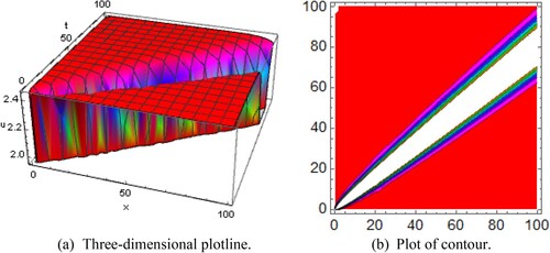$u_7(x,t)$, for $\mu =1,\beta =1,\alpha =\frac{1}{2}$ and $10\le x\le 1000,10\le t\le 1000$ (fractional Kelin–Gordon equation) recites double solitons solutions shown Figure 7. The behaviour of the shape of solution $u_7(x,t)$ is corresponding to the figure of solution $u_8(x,t),$ for $\mu =1,\beta =1,\alpha =\frac{1}{2}$ and $10\le x\le 1000,10\le t\le 100$ and for straightforwardness the quality of these accomplishment solutions is cropped here. $u_{12}(x,t)$ for $\mu =1,\beta =1,\alpha =\frac{1}{2}$ and $-10\le x\le 10,000,-10\le t\le 10,000$, recites singleton solution for Figure 8. The behaviour of the shape of solution $u_7(x,t)$ is corresponding to figure of solution $u_{17}(x,t),$ for $\mu =1,\beta =1,\alpha =\frac{1}{2}$ and $0\le x\le 100,0\le t\le 100$, $u_{19}(x,t),$ for $\mu =1,\beta =1,\alpha =\frac{1}{2}$ and $0\le x\le 100,0\le t\le 100$, $u_{20}(x,t),$ for $\mu =1,\beta =1,\alpha =\frac{1}{2}$ and $0\le x\le 100,0\le t\le 100$, hence for straightforwardness the quality of these accomplishment solutions is cropped here. $u_{15}(x,t)$ for $\mu =1,\beta =1,\alpha =\frac{1}{2}$ and $0\le x\le 10,0\le t\le 10$, $u_{16}(x,t)$ for $\mu =1,\beta =1,\alpha =\frac{1}{2}$ and $0\le x\le 0.5,0\le t\le 0.5$ performs king shape solution for Figure 9, and Figure 10.$u_{18}(x,t)$ for $\mu =1,\beta =1,\alpha =\frac{1}{2}$ and $0\le x\le 100,0\le t\le 100$ performs singular king shape wave solution depicted by Figure 11. Finally, $u_{22}(x,t)$ for $\mu =1,\beta =1,\alpha =\frac{1}{2}$ and $0\le x\le 10,0\le t\le 10$, performs anti-double king shape solution for Figure 12.

Figure 1. Diagram of the periodic king shape wave solution $u_1(x,t)$, representing (a) the three-dimensional plotline (b) plot of contour with the interval $0<x<10$ and $0<t<10$.

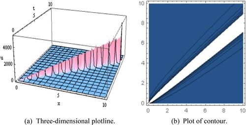
Figure 2. Diagram of the multiple soliton shape wave solution $u_2(x,t)$, representing (a) the three-dimensional plotline (b) plot of contour with the interval $-700<x<.5$ and $-700<t<.5$.

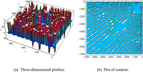
Figure 3. Diagram of the anti-bell shape wave solution $u_3(x,t)$ representing (a) the three-dimensional plotline (b) plot of contour with the interval $0<x<10$ and $0<t<10$.

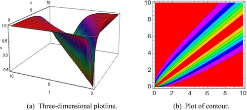
Figure 4. Diagram of the periodic-bell shape wave solution $u_4(x,t)$, representing (a) the three-dimensional plotline (b) plot of contour with the interval $10<x<100$ and $10<t<100$.

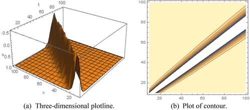
Figure 5. Diagram of the periodic-bell shape wave solution $u_{10}(x,t)$, representing (a) the three-dimensional plotline (b) plot of contour with the interval $0<x<10$ and $0<t<10$.

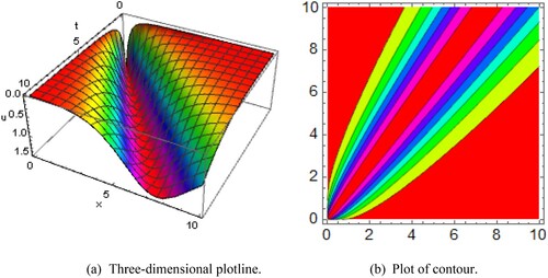
Figure 6. Diagram of the anti-periodic king shape wave solution $u_5(x,t)$ representing (a) the three-dimensional plotline (b) plot of contour and with the interval $0<x<100$ and $0<t<100$.

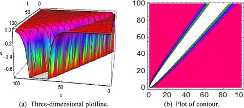
Figure 7. Diagram of the double soliton shape wave solution $u_7(x,t)$ representing (a) the three-dimensional plotline (b) plot of contour with the interval $10<x<1000$ and $10<t<1000.$

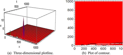
Figure 8. Diagram of the single soliton wave solution $u_{12}(x,t)$ representing (a) the three-dimensional plotline (b) plot of contour with the interval $-10<x<10000$ and $-10<t<10000$.

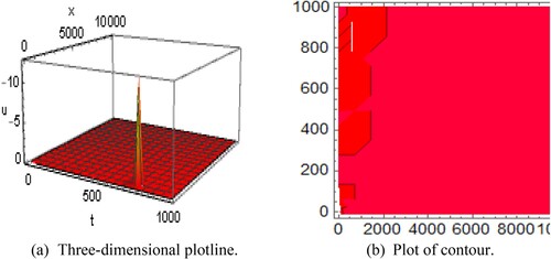
Figure 9. Diagram of the king shape wave solution $u_{15}(x,t)$ representing (a) the three-dimensional plotline (b) plot of contour with the interval $0<x<10$ and $0<t<10$.

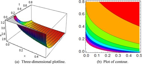
Figure 10. Diagram of the king shape wave solution $u_{16}(x,t)$ representing (a) the three-dimensional plotline (b) plot of contour with the interval $0<x<0.5$ and $0<t<0.5$.

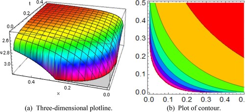
Figure 11. Diagram of the singular kink shape wave solution $u_{18}(x,t)$ representing (a) the three-dimensional plotline (b)plot of contour with the interval $0<x<100$ and $0<t<100$.

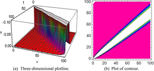
Figure 12. Diagram of the anti-double king shape wave solution $u_{22}(x,t)$, representing (a) the three-dimensional plotline (b) plot of contour with the interval $0<x<10$ and $0<t<10$.

6. Comparison of results

This sub-section represents some of the obtained solutions, which are strongly similarities with the solutions that were previously established and displayed in Table 1 and Table 2, respectively. The existing literature contains different types of methods to solve these mentioned equations, including confirmable derivative. It is interesting to observe that some of our achieved solutions have shown good similarity to Lu [36] for the definite values of arbitrary constant.

Table 1. Comparison between Lu [36] and our achieved solutions.

Lu [36]	Obtained solutions
If a $=1,c=1,\lambda =2,{\zeta }_0=1\text{and}l=1$ then (26) solution becomes $u_{5,6}(x,t)=\sqrt{-1}\text{tan}\text{h}\left(\sqrt{{\displaystyle \frac{-1}{6}}}\left(x-{\displaystyle \frac{4\sqrt{t}}{.5\sqrt{\pi }}}+1\right)\right)$	$k={\displaystyle \frac{1}{2}}{\displaystyle \frac{\sqrt{p+4l^2{\mu }^2}}{\mu }}$, $l=l$, $a_0=-{\displaystyle \frac{1}{2}}{\displaystyle \frac{p}{q}},a_1=0,a_2=0,$ and $b_1=0,b_2={\displaystyle \frac{3}{2}}{\displaystyle \frac{p}{q}}$, then (12) becomes $u_1(x,t)=-{\displaystyle \frac{1}{2}}+{\displaystyle \frac{3}{2}}\text{cot}{\text{h}}^2\left(2\sqrt{x}-\sqrt{5t}\right)$
If a $=1,c=1,\lambda =2,{\zeta }_0=1\text{and}l=1$ then (2) solution becomes $u_{7,8}(x,t)=\sqrt{-1}\text{cot}\text{h}\left(\sqrt{{\displaystyle \frac{-1}{6}}}\left(x-{\displaystyle \frac{4\sqrt{t}}{.5\sqrt{\pi }}}+1\right)\right)$	$k={\displaystyle \frac{1}{2}}{\displaystyle \frac{\sqrt{p+4l^2{\mu }^2}}{\mu }}$, $l=l$, $a_0=-{\displaystyle \frac{1}{2}}{\displaystyle \frac{p}{q}},a_1=0,a_2={\displaystyle \frac{3}{2}}{\displaystyle \frac{p}{q}}$ and $b_1=0,b_2=0$ then (14) becomes $u_3(x,t)=-{\displaystyle \frac{1}{2}}+{\displaystyle \frac{3}{2}}\text{tan}{\text{h}}^2\left(2\sqrt{x}-\sqrt{5t}\right)$

Table 2. Comparison between Guner et al. [51] and our obtained solutions.

Guner et al. [51]	Obtained solutions
If $A=1,k_1=1,x_1=1,\alpha =1\text{and}\sigma =1$ then (40) solution becomes $u(x,t)=\text{tan}\text{h}\left({\displaystyle \frac{\sqrt{6}}{2}}{\displaystyle \frac{\sqrt{t}}{.5\sqrt{\pi }}}+{\displaystyle \frac{\sqrt{x_1}}{.5\sqrt{\pi }}}\right)$	$\delta ={\displaystyle \frac{1}{2}}{\displaystyle \frac{\sqrt{-2+4{\upsilon }^2{\mu }^2}}{\mu }}$, $\nu =\nu$, $a_0=0,a_1=\sqrt{6},$ and $b_1=0$. Then (36) becomes $u_{21}(x,t)=\sqrt{6}\tan h\left(\sqrt{2}\sqrt{x}+2\sqrt{t}\right)$
If $A=1,k_1=1,x_1=1,\alpha =1\text{and}\sigma =1$ then (41) solution becomes $u(x,t)=\text{sec}\text{h}\left({\displaystyle \frac{\sqrt{6}}{2}}{\displaystyle \frac{\sqrt{t}}{.5\sqrt{\pi }}}+{\displaystyle \frac{\sqrt{x_1}}{.5\sqrt{\pi }}}\right)$	$\delta ={\displaystyle \frac{1}{2}}{\displaystyle \frac{\sqrt{-2+4{\upsilon }^2{\mu }^2}}{\mu }}$, $\nu =\nu$, $a_0=0,a_1=\sqrt{6},$ and $b_1=0$. Then (37) becomes $u_{22}(x,t)=\sqrt{6}\sqrt{1-\text{sec}\text{h}{\left(\sqrt{2}\sqrt{x}+2\sqrt{t}\right)}^2}$

For the upstairs tables, the hyperbolic function solutions are comparable and are indistinguishable in the case that we set definite values of the arbitrary constants. It is significant to recognize that the space-time fractional Kelin–Gordon equation’s travelling wave solutions $u_1(x,t)$ $u_2(x,t)$, $u_4(x,t),u_5(x,t),$ $u_7(x,t),$ $u_{10}(x,t)$, $u_{12}(x,t)$, are completely innovative. It is also relevant to point out that they were not enclosed in prior exertion.

For the upstairs tables, the hyperbolic function solutions are comparable and are indistinguishable in the case that we set definite values of the arbitrary constants. It is significant to recognize that the space-time fractional Sine-Gordon equation’s travelling wave solutions $u_{15}(x,t)$, $u_{16}(x,t),u_{18}(x,t),$ $u_{22}(x,t)$ are completely new. It is also relevant to point out that they were not enclosed in a prior study.

7. Conclusion

The exact solutions of the space-time fractional Klein–Gordon equation and the fractional Sine-Gordon equation is in the most general form have been obtained using a direct analytic method based on the extended tanh-function in this study. The recommended method is extremely effective, reliable, and powerful. Linearization, perturbation, starting, and boundary conditions are not required, which is one of the method’s advantages. Because that both time and space are fractional, the suggested method is further general than the other. From those two equations, we have attained some new and additional travelling wave solutions to the FNLPDEs. The proposed method and well-informed solitons are used to create these two equations for specified values of parameters such as king type, periodic king shape single soliton, double solitons, multiple solitons, bell shape wave solutions, and so on. Besides the solutions are sketched in 3D, and contour patterns. It is worth mentioning that all derived solutions are checked for accuracy by replacing them directly with the original equations. For comprehensive research and innovation, these types of studies are highly suggested. To the best of our consciousness, it is mentionable that the new type of acquired results in this learning has not been accomplished previously. Furthermore, the proficient solutions sanction that the anticipated process affords an effective mathematical implement also seems to be sturdier, relaxed, stronger, and quicker employing the symbolic program computation system. After all, the dissimilar types of new exact wave solutions conquered in this paper might have a vital role for future research in the territory of mathematical physics and those types of phenomena are only achieved by using the fractional Klein–Gordon equation and Sine-Gordon equation.

Disclosure statement

No potential conflict of interest was reported by the author(s).

References

- Du M, Wang Z, Hu H. Measuring memory with the order of fractional derivative. Sci Rep. 2013;3:1–3. DOI:10.1038/srep03431
- Caputo M, Fabrizio M. A new definition of fractional derivative without singular kernel. Prog Fract Differ Appl. 2015;1:73–85. DOI:10.12785/pfda/010201
- Zheng B. Exp-function method for solving fractional partial differential equations. Sci World J. 2013;2013; DOI:10.1155/2013/465723
- Čermák J, Kisela T. Stability properties of two-term fractional differential equations. Nonlinear Dyn. 2015;80:1673–1684. DOI:10.1007/s11071-014-1426-x
- Gomez CA, Jhangeer A, Rezazadeh H, et al. Closed form solutions of the perturbed Gerdjikov-Ivanov equation with variable coefficients. East Asian J Appl Math. 2021;11(1):207–218.
- Manafian J, Ilhan OA, Mohammed SA. Forming localized waves of the nonlinearity of the DNA dynamics arising in oscillator-chain of Peyrard-Bishop model. AIMS Math. 2020;5(3):2461–2483.
- Manafian J. On the complex structures of the Biswas-Milovic equation for power, parabolic and dual parabolic law nonlinearities. Eur Phys J Plus. 2015;130(12):1–20.
- Dehghan M, Manafian J, Saadatmandi A. Analytical treatment of some partial differential equations arising in mathematical physics by using the exp-function method. Int J Mod Phys B. 2011;25(22):2965–2981.
- Hosseini K, Mirzazadeh M, Gómez-Aguilar JF. Soliton solutions of the Sasa–Satsuma equation in the monomode optical fibers including the beta-derivatives. Optik. 2020;224:165425.
- Hosseini K, Kaur L, Mirzazadeh M, et al. 1-soliton solutions of the (2 + 1)-dimensional Heisenberg ferromagnetic spin chain model with the beta time derivative. Opt Quantum Electron. 2021;53(2):1–10.
- Meng F. A new approach for solving fractional partial differential equations. J Appl Math. 2013;2013. DOI:10.1155/2013/256823
- Li C, Chen A, Ye J. Numerical approaches to fractional calculus and fractional ordinary differential equation. J Comput Phys. 2011;230:3352–3368. DOI:10.1016/j.jcp.2011.01.030
- Varieschi GU. Applications of fractional calculus to Newtonian mechanics. J Appl Math Phys. 2018;06:1247–1257. DOI:10.4236/jamp.2018.66105
- Leta TD, Liu W, El Achab A, et al. Dynamical behavior of traveling wave solutions for a (2 + 1)-dimensional Bogoyavlenskii coupled system. Qual Theory Dyn Syst. 2021;20(1):1–22.
- Huang Q, Huang G, Zhan H. A finite element solution for the fractional advection-dispersion equation. Adv Water Resour. 2008;31:1578–1589. DOI:10.1016/j.advwatres.2008.07.002
- Ilhan OA, Manafian J, Alizadeh AA, et al. New exact solutions for nematicons in liquid crystals by the tan(ϕ/2)-expansion method arising in fluid mechanics. Eur Phys J Plus. 2020;135(3):1–19.
- Manafian J. Optical soliton solutions for Schrödinger type nonlinear evolution equations by the tan (Φ (ξ)/2)-expansion method. Optik. 2016;127(10):4222–4245.
- Odibat Z, Momani S. A generalized differential transform method for linear partial differential equations of fractional order. Appl Math Lett. 2008;21:194–199. DOI:10.1016/j.aml.2007.02.022
- Lu Q, Ilhan OA, Manafian J, et al. Multiple rogue wave solutions for a variable-coefficient Kadomtsev–Petviashvili equation. Int J Comput Math. 2021;98(7):1457–1473.
- Tala-Tebue E, Korkmaz A, Rezazadeh H, et al. New auxiliary equation approach to derive solutions of fractional resonant Schrödinger equation. Anal Math Phys. 2021;11(4):1–13.
- Hosseini K, Mirzazadeh M, Ilie M, et al. Biswas–Arshed equation with the beta time derivative: optical solitons and other solutions. Optik. 2020;217:164801.
- Jafari H, Seifi S. Homotopy analysis method for solving linear and nonlinear fractional diffusion-wave equation. Commun Nonlinear Sci Numer Simul. 2009;14:2006–2012. DOI:10.1016/j.cnsns.2008.05.008
- Rezazadeh H, Younis M, Eslami M, et al. New exact traveling wave solutions to the (2 + 1)-dimensional chiral nonlinear Schrödinger equation. Math Model Nat Phenom. 2021;16:38.
- Uddin MH, Khatun MA, Arefin MA, et al. Abundant new exact solutions to the fractional nonlinear evolution equation via Riemann-Liouville derivative. Alexandria Eng J. 2021;60. DOI:10.1016/j.aej.2021.04.060
- Raslan KR, Ali KK, Shallal MA. The modified extended tanh method with the Riccati equation for solving the space-time fractional EW and MEW equations. Chaos, Solitons Fractals. 2017;103:404–409.
- Uddin MH, Arefin MA, Akbar MA. New explicit solutions to the fractional-order Burgers equation. Math Probl Eng. 2021;2021:Article ID 6698028.
- Hashemi MS, Rezazadeh H, Almusawa H, et al. A Lie group integrator to solve the hydromagnetic stagnation point flow of a second grade fluid over a stretching sheet. AIMS Math. 2021;6(12):13392–13406.
- Manafian J, Ilhan OA, Ali KK, et al. Cross-kink wave solutions and semi-inverse variational method for (3 + 1)-dimensional potential-YTSF equation. East Asian J Appl Math. 2020;10(3):549–565.
- Mophou GM. Existence and uniqueness of mild solutions to impulsive fractional differential equations. Nonlinear Anal Theory Methods Appl. 2010;72:1604–1615. DOI:10.1016/j.na.2009.08.046
- Liu F, Anh V V, Turner I, et al. Time fractional advection-dispersion equation. J Appl Math Comput. 2003;13:233–245. DOI:10.1007/BF02936089
- Jiang W, Lin Y. Approximate solution of the fractional advection-dispersion equation. Comput Phys Commun. 2010;181:557–561. DOI:10.1016/j.cpc.2009.11.004
- Pandey RK, Singh OP, Baranwal VK. An analytic algorithm for the space-time fractional advection-dispersion equation. Comput Phys Commun. 2011;182:1134–1144. DOI:10.1016/j.cpc.2011.01.015
- Xue C, Nie J, Tan W. An exact solution of start-up flow for the fractional generalized Burgers’ fluid in a porous half-space. Nonlinear Anal Theory Methods Appl. 2008;69:2086–2094. DOI:10.1016/j.na.2007.07.047
- Molliq R Y, Noorani MSM, Hashim I. Variational iteration method for fractional heat- and wave-like equations. Nonlinear Anal Real World Appl. 2009;10:1854–1869. DOI:10.1016/j.nonrwa.2008.02.026
- Golmankhaneh AK, Golmankhaneh AK, Baleanu D. On nonlinear fractional KleinGordon equation. Signal Process. 2011;91:446–451. DOI:10.1016/j.sigpro.2010.04.016
- Lu B. The first integral method for some time fractional differential equations. J Math Anal Appl. 2012;395:684–693. DOI:10.1016/j.jmaa.2012.05.066
- Gepreel KA, Mohamed MS. Analytical approximate solution for nonlinear space – time fractional Klein–Gordon equation. Chinese Phys B. 2013;22; DOI:10.1088/1674-1056/22/1/010201
- Jafari H, Tajadodi H, Kadkhoda N, et al. Fractional subequation method for Cahn-Hilliard and Klein-Gordon equations. Abstr Appl Anal. 2013;2013; DOI:10.1155/2013/587179
- Ran M, Zhang C. Compact difference scheme for a class of fractional-in-space nonlinear damped wave equations in two space dimensions. Comput Math with Appl. 2016;71:1151–1162. DOI:10.1016/j.camwa.2016.01.019
- Wang Q, Chen Y, Zhang H. A new Riccati equation rational expansion method and its application to (2 + 1)-dimensional Burgers equation. Chaos Solitons Fractals. 2005;25:1019–1028. DOI:10.1016/j.chaos.2005.01.039
- Abdel-Salam EAB, Gumma EAE. Analytical solution of nonlinear space-time fractional differential equations using the improved fractional Riccati expansion method. Ain Shams Eng J. 2015;6:613–620. DOI:10.1016/j.asej.2014.10.014
- Sirendaoreji. Unified Riccati equation expansion method and its application to two new classes of Benjamin–Bona–Mahony equations. Nonlinear Dyn. 2017;89:333–344. DOI:10.1007/s11071-017-3457-6
- Shallal MA, Jabbar HN, Ali KK. Analytic solution for the space-time fractional Klein-Gordon and coupled conformable Boussinesq equations. Results Phys. 2018;8:372–378. DOI:10.1016/j.rinp.2017.12.051
- Unsal O, Guner O, Bekir A. Analytical approach for space–time fractional Klein–Gordon equation. Optik (Stuttg). 2017;135:337–345. DOI:10.1016/j.ijleo.2017.01.072
- Zhou Q, Ekici M, Mirzazadeh M, et al. The investigation of soliton solutions of the coupled sine-Gordon equation in nonlinear optics. J Mod Opt. 2017;64:1677–1682. DOI:10.1080/09500340.2017.1310318
- Hosseini K, Mayeli P, Kumar D. New exact solutions of the coupled sine-Gordon equations in nonlinear optics using the modified Kudryashov method. J Mod Opt. 2018;65:361–364. DOI:10.1080/09500340.2017.1380857
- Khalil R, Al Horani M, Yousef A, et al. A new definition of fractional derivative. J Comput Appl Math. 2014;264:65–70. DOI:10.1016/j.cam.2014.01.002
- Wazwaz AM. The extended tanh method for abundant solitary wave solutions of nonlinear wave equations. Appl Math Comput. 2007;187:1131–1142. DOI:10.1016/j.amc.2006.09.013
- Gepreel KA, Mohamed MS. Analytical approximate solution for nonlinear space–time fractional Klein–Gordon equation. Chinese Phys. B. 2013;22:010201
- Barone A, Esposito F, Magee CJ, et al. Theory and applications of the sine-gordon equation. La Rivista del Nuovo Cimento. 1971;1:227–267. DOI:10.1007/BF02820622
- Guner O, Bekir A, Korkmaz A. Tanh-type and sech-type solitons for some space-time fractional PDE models. Eur Phys J Plus. 2017;132(2):1–12.