Numerical study on mean flow characteristics for a combined turbulent wall and offset jets with a parallel co-flow

Abstract

Combined turbulent wall and offset jets with and without the presence of a parallel co-flow stream are investigated using the k-ω turbulence model. We focus on the effects of co-flow velocity on the locations of various characteristic points formed owing to the interaction of wall and offset jets in the dual jet flow. The inlet Reynolds number is taken as 15,000 and the offset ratio is varied from 5 to 11. At low offset ratios, the co-flow velocity effect remains almost negligible. With the progressive increase in co-flow velocity, the characteristic points are gradually relocated towards the further downstream direction with a transverse movement away from the bottom wall whose effect is weakened with the increase in co-flow velocity. Furthermore, regression analysis shows power law and linear correlations of the longitudinal and transverse coordinates of characteristic points with the co-flow velocity and the offset ratio.

KEYWORDS:

• Wall jet
• offset jet
• co-flow velocity
• CFD
• turbulence

1. Introduction

In the case of environmental flows, turbulent jets are generally found accompanied by a stream of co-flow in the direction parallel to the jet. The most common example is the disposal of wastewater into rivers and marines. Flow geometries in such applications resemble a flow of a combined wall and offset jets (or dual jet) accompanied by a parallel co-flow which is the focus of the present study.

When a stream of fluid is ejected from a nozzle parallel to a solid wall, a wall jet is generated. Many authors studied the flow characteristics of a two-dimensional plane wall jet, for example, Forthmann [1], Myers et al. [2], Gutmark and Wygnanski [3], Launder and Rodi [4], Abrahamssonet al. [5], Schneider and Goldstein [6], Eriksson et al. [7], George et al. [8], Dejoan and Leschziner [9], Ahlman et al. [10], Azim [11] and Wei et al. [12]. An offset jet occurs when a stream of fluid is ejected from a nozzle kept a certain height from the solid wall. A detailed discussion on a two-dimensional offset jet flow can be found in Bourque and Newman [13], Sawyer [14] and [15], Pelfrey and Liburdy [16] and [17], Koo and Park [18], Gu [19], Kim et al. [20] and Gao and Ewing [21], Rathore and Das [22] and Singh et al. [23].

Compared to either a single wall jet or a single offset jet, the studies on a combined flow of wall and offset jets are less available in the literature. Wang and Tan [24] undertook a pioneering work on such flow configuration. They designated the combined flow of wall and offset jets as dual jet. They experimentally found an unsteady von-Karman like vortex structures in the near flow field when the offset ratio OR = or/w  = 2, where h denotes the dimensional offset height and w the width of the offset jet. A couple of years later, Kumar and Das [25] solved the Reynolds Averaged Navier-Stokes equations (RANS) for modelling a dual jet with OR = 9. Further, with the same geometric condition i.e. OR = 2 adopted in Wang and Tan [24], Li et al. [26] numerically simulated the dual jet using the large eddy simulation (LES) method. They obtained the mean flow results for the decay of maximum mean streamwise velocity, the growth of the jet width, and the mean streamwise velocity profiles at different downstream locations, and validated these results with the experimental data of Wang and Tan [24]. The rest of the results include the statistical analysis of velocity fluctuations and dilution characteristics of the dual jet.

Following the work of Wang and Tan [24], Mondal et al. [27] explored the effect of offset ratio on the von-Karman like unsteady phenomenon and found the occurrence of vortex shedding only within the range OR = 1.7–3.1. Subsequently, they also examined the effects of jet width on the same unsteady behaviour and their results detected a periodic vortex shedding if the width to offset height ratio is kept in the range 0.2 and 2 [28]. Afterwards, they varied the velocity ratio of the offset jet to the wall jet, a periodic large-scale von Karman-like vortex street in the flow field was identified for the velocity ratio in the range 0.78–1.34 [29].

A numerical analysis was performed by Kumar [30] to compare the flow characteristic of an offset jet with those of dual jet for the offset ratio OR in the range 3–15. Correlations that predicted the longitudinal and transverse positions of the merge point, combined point and the recirculation vortex centres were provided as a function of OR. In a numerical simulation, Nidhal et al. [31] conducted a parametric study on the dual jet considering the effects of the inlet velocity ratio on the mean flow field of dual jet. They also investigated the effect of the offset jet ejection angle on the dual jet [32]. In both the studies, they found that the acceleration of merging process of two jets increases with increasing either the velocity ratio or the ejection angle of the offset jet.

Recently, Assoudi et al. [33] numerically investigated fluid flow and thermal characteristics for a dual jet using the standard k-ε and Reynolds-stress models by varying the offset ratio, velocity ratio, and temperature jet exit ratio. They found that the results of the Reynolds-stress model were closer to the experimental results of Wang and Tan [24] as compared to those by the standard k-ε model. Also, they found that the thermal and fluid flow characteristics had the effect of a parallel flowing wall jet.

The above review of literature insinuates that past studies on dual jet primarily focus on variation of either geometric parameters (i.e. intermediate distance between wall and offset jets, and jet width) or inlet parameters (jet inlet velocity, and jet ejection angle). However, to the best of the authors’ knowledge, the study pertinent to the dual jet coupled with a co-flow is not traceable in the literature. According to the study of Ayech et al. [34], the flow structure of a wall jet is considerably affected by the presence of a stream of co-flow. Similarly, the presence of co-flow in a combined wall jet and offset jet is expected to alter the mean flow structure quite substantially. Therefore, in the current work, an endeavour is made to investigate the effects co-flow velocity on the mean flow characteristics of dual jet associated with a parallel co-flow. A special emphasis is given on the displacements of various tocharacteristic points (merging point, combined point and upper and lower vortex centres) as a result of variation in co-flow velocity. It is relevant to mention here that the present study is the first work on dual jet dealing with the co-flow stream, establishing correlation functions for the axial and transverse (lateral) locations of the characteristic points in terms of the co-flow velocity and the offset ratio.

The output of the present study will provide a rough estimate of the locations of various characteristic points present in the flow field of the dual jet flow without having to perform the CFD (Computational Fluid Dynamics) simulation, which may be useful in applications related to discharge flows in wastewater disposal systems. In the current study, the computational simulations are carried out using RANS utilizing the Wilcox k-ω turbulence model. The computational results are shown for the % of co-flow velocity (CFV) with respect to the jet velocity in the range CFV = 0–40%, offset ratio in the range OR = or/w = 5–11 and the Reynolds number Re = 15,000 (where, $\text{CFV}=\frac{{\text{u}}_{\text{CF}}}{{\text{u}}_0}\times 100$, $\text{OR}=\frac{\text{or}}{\text{w}}$, $Re=\frac{{\text{u}}_{\text{o}}\text{w}}{\upsilon }$, $u_{CF}$ and $u_0$ being the co-flow velocity and the jet inlet velocity, respectively). The axial and transverse evolution of different parameters are plotted with respect to the non-dimensional axial X = x/w and transverse Y = y/w coordinates. Note that w presents the nozzle width as noted above.

2. Mathematical formulation

Figure 1 represents a schematic diagram for a combined two-dimensional flow configuration of a wall jet and an offset jet with a parallel co-flow just above the offset jet. Here, the lower jet is the wall jet and the upper one is the offset jet. Two turbulent jets with same inlet velocity $u_0$ and width $w$ are ejected from the two identical nozzles with height of the lower boundary of the offset jet nozzle from the horizontal wall i.e.$y=0$. At the inlet of the flow domain, the velocity of the co-flow $u_{CF}$ is kept lower than the jet inlet velocity. The nozzle exit plane is represented by the y axis i.e. $x=0$.

Figure 1. Schematic flow configuration of a combined wall and offset jets.

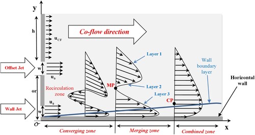
Since the entrainment of the wall jet is blocked by the offset jet, the two jets begin to approach (move closer) each other after issuing from the nozzle and eventually they merge at the merge point (MP). This phenomenon is commonly known as the Coanda effect [29]. Further downstream of the merge point MP, interaction of merged jets persists until the combined point CP where the flow is seen to be more similar to that of the wall jet. Several flow zones are formed in the dual jet flow: converging zone (between MP and the nozzle exit plane i.e.$x=0$), merging zone (between MP and CP) and combined zone (downstream of CP or rest of the flow domain).

2.1. Geometric configuration

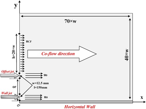
Figure 2 shows the geometric configurations of combined wall and offset jet flow adopted for the present computational study. The nozzles width and length are taken $w=12.5\text{mm}$ and $l=150\text{mm}$, respectively. The co-flow is ejected parallel to the discharge of the main jets and located just above the offset jet nozzle. The height of the co-flow stream from the upper boundary of the offset jet nozzle is kept always fixed at $or=20\times w$, whereas the offset ratio and the co-flow velocity, respectively, are varied in the range $\text{OR}=5-11$ and $\text{CFV}=0\mathrm{\%}-40\mathrm{\%}$. The total dimension of the computational domain is taken as $70w\times 40w$ (along the x and y, respectively) accommodating the dual jet and the development of the flow throughout the domain. First of all, the present numerical model is validated on the geometric configuration of Pelfray and Liburdy [16] for single offset jet (zero wall jet velocity) without co-flow (CFV = 0%) and for an offset ratio OR = 6.5. For the rest of calculations, geometric configuration of combined wall and offset jet flow is considered to study the effect of co-flow on the mean flow behaviours.

Figure 2. Geometric configuration and numerical model of combined wall and offset jets.

2.2. Governing equations

Turbulent flow under the present study is considered as two-dimensional (2D) and steady; the fluid is assumed as incompressible without the presence of body forces. The RANS method is used for numerical modelling. According to Figure 2, the length of the nozzle (l = 150 mm) is considered to be much larger than its width (w = 12.5 mm). Therefore, the influence of spanwise direction (z direction) can be ignored to ensure the flow to be 2D. For turbulence closure, the two-equation Wilcox k-ω turbulence model is utilized. The dimensional form of governing equations for the k-ω based RANS can be written in Cartesian tensor representation as follows: (1) $\begin{array}{rl}& \frac{\mathrm{\partial }}{\mathrm{\partial }{x}_i}(\rho u_i)=0\end{array}$(1) (2) $\begin{array}{rl}& \frac{\mathrm{\partial }}{\mathrm{\partial }{x}_j}(\rho u_i{u}_j)=-\frac{\mathrm{\partial }p}{\mathrm{\partial }{x}_i}+\frac{\mathrm{\partial }}{\mathrm{\partial }{x}_j}\left[\mu \left(\frac{\mathrm{\partial }{u}_i}{\mathrm{\partial }{x}_j}+\frac{\mathrm{\partial }{u}_j}{\mathrm{\partial }{x}_i}-\frac{2}{3}{\delta }_{ij}\frac{\mathrm{\partial }{u}_l}{\mathrm{\partial }{x}_l}\right)\right]\\ & +\frac{\mathrm{\partial }}{\mathrm{\partial }{x}_j}(-\rho \overline{u_i^{\mathrm{\prime }}{u}_j^{\mathrm{\prime }}})\end{array}$(2) To close Equation 2(2) $\begin{array}{rl}& \frac{\mathrm{\partial }}{\mathrm{\partial }{x}_j}(\rho u_i{u}_j)=-\frac{\mathrm{\partial }p}{\mathrm{\partial }{x}_i}+\frac{\mathrm{\partial }}{\mathrm{\partial }{x}_j}\left[\mu \left(\frac{\mathrm{\partial }{u}_i}{\mathrm{\partial }{x}_j}+\frac{\mathrm{\partial }{u}_j}{\mathrm{\partial }{x}_i}-\frac{2}{3}{\delta }_{ij}\frac{\mathrm{\partial }{u}_l}{\mathrm{\partial }{x}_l}\right)\right]\\ & +\frac{\mathrm{\partial }}{\mathrm{\partial }{x}_j}(-\rho \overline{u_i^{\mathrm{\prime }}{u}_j^{\mathrm{\prime }}})\end{array}$(2) , the Reynolds stress term $-\overline{\rho u_i^{\mathrm{\prime }}{u}_j^{\mathrm{\prime }}}$ can be approximated using Boussinesq hypothesis which relates the Reynolds stress with the mean velocity gradient as follows: (3) $-\rho \overline{u_i^{\mathrm{\prime }}{u}_j^{\mathrm{\prime }}}={\mu }_t\left(\frac{\mathrm{\partial }{u}_i}{\mathrm{\partial }{x}_j}+\frac{\mathrm{\partial }{u}_j}{\mathrm{\partial }{x}_i}\right)-\frac{2}{3}\left(\rho k+{\mu }_t\frac{\mathrm{\partial }{u}_k}{\mathrm{\partial }{x}_k}\right){\delta }_{ij}$(3) The turbulent kinetic energy k and the rate of specific dissipation of turbulent kinetic energy ω are expressed in Equation 4(4) $\begin{array}{r}\frac{\mathrm{\partial }}{\mathrm{\partial }{x}_i}(\rho k{u}_i)=\frac{\mathrm{\partial }}{\mathrm{\partial }{x}_j}\left({\mathrm{\Gamma }}_k\frac{\mathrm{\partial }k}{\mathrm{\partial }{x}_j}\right)+G_k-Y_k+S_k\end{array}$(4) and Equation 5(5) $\begin{array}{r}\frac{\mathrm{\partial }}{\mathrm{\partial }{x}_i}(\rho \omega u_i)=\frac{\mathrm{\partial }}{\mathrm{\partial }{x}_j}\left({\mathrm{\Gamma }}_w\frac{\mathrm{\partial }\omega }{\mathrm{\partial }{x}_j}\right)+G_{\omega }-Y_{\omega }+S_{\omega }\end{array}$(5) , respectively. (4) $\begin{array}{r}\frac{\mathrm{\partial }}{\mathrm{\partial }{x}_i}(\rho k{u}_i)=\frac{\mathrm{\partial }}{\mathrm{\partial }{x}_j}\left({\mathrm{\Gamma }}_k\frac{\mathrm{\partial }k}{\mathrm{\partial }{x}_j}\right)+G_k-Y_k+S_k\end{array}$(4) (5) $\begin{array}{r}\frac{\mathrm{\partial }}{\mathrm{\partial }{x}_i}(\rho \omega u_i)=\frac{\mathrm{\partial }}{\mathrm{\partial }{x}_j}\left({\mathrm{\Gamma }}_w\frac{\mathrm{\partial }\omega }{\mathrm{\partial }{x}_j}\right)+G_{\omega }-Y_{\omega }+S_{\omega }\end{array}$(5) In Equation 4(4) $\begin{array}{r}\frac{\mathrm{\partial }}{\mathrm{\partial }{x}_i}(\rho k{u}_i)=\frac{\mathrm{\partial }}{\mathrm{\partial }{x}_j}\left({\mathrm{\Gamma }}_k\frac{\mathrm{\partial }k}{\mathrm{\partial }{x}_j}\right)+G_k-Y_k+S_k\end{array}$(4) and Equation 5(5) $\begin{array}{r}\frac{\mathrm{\partial }}{\mathrm{\partial }{x}_i}(\rho \omega u_i)=\frac{\mathrm{\partial }}{\mathrm{\partial }{x}_j}\left({\mathrm{\Gamma }}_w\frac{\mathrm{\partial }\omega }{\mathrm{\partial }{x}_j}\right)+G_{\omega }-Y_{\omega }+S_{\omega }\end{array}$(5) , the terms G_k and G_ω denote the generation of k and ω, respectively. ${\mathrm{\Gamma }}_k$ and ${\mathrm{\Gamma }}_{\omega }$ correspond the effective diffusivity for k and ω, respectively. Y_k and Y_ω represent the dissipation of k and ω, respectively; S_k and S_ω being the source terms. The k-ω turbulence model details is available on ANSYS, Inc. (2019) ANSYS Fluent User’s Guide, Release 19.0

2.3. Grid generation and boundary conditions

As clearly shown in Figure 3, a uniform mesh is adopted along the offset jet, the wall jet, the co-flow and the nozzles spacing with mesh spacing a = 0.08. For the lateral side, along the vertical direction, the mesh is non uniform with spacing a = 0.3 and an expansion ratio e = 1.05. For the horizontal wall, the mesh spacing, and the expansion ratio is 0.3 and 1.01, respectively. Note that all the opposite segments have the same grid size details.

Figure 3. Grid layout of computational domain together with boundary conditions.

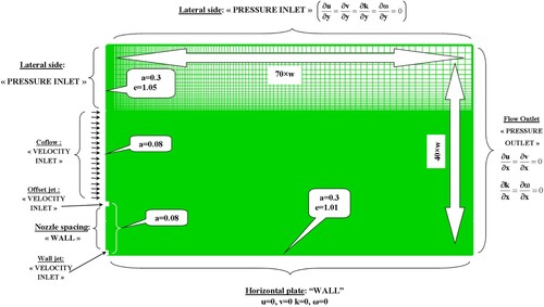
A uniform velocity profile is adopted along the wall jet, the offset jet as well as the co-flow which is labelled “VELOCITY INLET boundary condition”. Along the horizontal plate and the nozzle spacing, no slip boundary condition with zero velocity along the axial and transverse direction which is described by “WALL boundary condition” in ANSYS solver. At the lateral side and the flow outlet, the pressure is supposed to be that of the ambient because the domain dimension is sufficiently wide to not affect the flow which is labelled as “PRESSURE INLET and PRESSURE OUTLET boundaries conditions” (Figure 3). Note that for the validation case (single offset jet without co-flow), no modification is performed on number of cells, the only modification concerns the boundary condition at the wall jet as well as on the co-flow (boundary condition changed from VELOCITY INLET to WALL). The boundary and inlet conditions are presented in Table 1. Note that in Table 1, $C_{\mu }=0.09$ is a constant value, D_h is the hydraulic diameter and l is the characteristics length (l = 0.07×D_h). The turbulent kinetic energy at the nozzle outlet as well as at the co-flow outlet is calculated based on the ejection velocity at the nozzles noted u₀ and at the co-flow noted u_CF. At the nozzles outlet the velocity is fixed to 17.4 m/s and at the co-flow, the outlet velocity depends on the co-flow intensity.

Table 1. Details of boundary conditions used.

Initial conditions	Details
Single offset jet
Offset jet inlet	Re = 15000	$k_0={\displaystyle \frac{3}{2}}(I{U}_0{)}^2=1.135{\displaystyle \frac{m^2}{s^2}}$
	u0 = 17.4 m/s
	I = 5%	${\omega }_0={\displaystyle \frac{k_0{r}^{\frac{1}{2}}}{{C_{\mu }}^{\frac{1}{4}}l}}=1203.1{\displaystyle \frac{1}{s}}$
	l = 0.07×Dh
Dual jet with co-flow
Offset jet inlet	Re = 15000	$k_0={\displaystyle \frac{3}{2}}(I{U}_0{)}^2=1.135{\displaystyle \frac{m^2}{s^2}}$
Wall jet inlet	u0 = 17.4 m/s
	I = 5%	${\omega }_0={\displaystyle \frac{{k_0}^{\frac{1}{2}}}{{C_{\mu }}^{\frac{1}{4}}l}}=1203.1{\displaystyle \frac{1}{s}}$
Coflow inlet	uCF = 1.74 m/s → UCF = 0.1 →CFV = 10%	$k_0=0.009{\displaystyle \frac{m^2}{s^2}}$
		${\omega }_0=13.6{\displaystyle \frac{1}{s}}$
	uCF = 3.48 m/s → UCF = 0.2	${\omega }_0=24.9{\displaystyle \frac{1}{s}}$
	→CFV = 20%	$k_0=0.032{\displaystyle \frac{m^2}{s^2}}$
	uCF = 5.22 m/s → UCF = 0.3 →CFV = 30%	$k_0=0.065{\displaystyle \frac{m^2}{s^2}}$
		${\omega }_0=35.4{\displaystyle \frac{1}{s}}$
	uCF = 6.96 m/s → UCF = 0.4 →CFV = 40%	$k_0=0.107{\displaystyle \frac{m^2}{s^2}}$
		${\omega }_0=45.6{\displaystyle \frac{1}{s}}$

2.4. Numerical schemes and methodologies

To solve the governing equations (Equations 1–5), the CFD (Computational Fluid Dynamics) software “ANSYS FLUENT” is utilized. The CDS (central difference scheme) is used to discretize the diffusive terms and the second order UPWIND scheme is used to discretize the convective terms. For pressure-velocity coupling, the SIMPLEC algorithm is used. The disposal method of Gauss-Seidel associated with a relaxation technique is used to solve the resulting tri-diagonal matrix. The convergence criterion is set as 10⁻⁵.

2.5. Grid independence test and velocity field validation

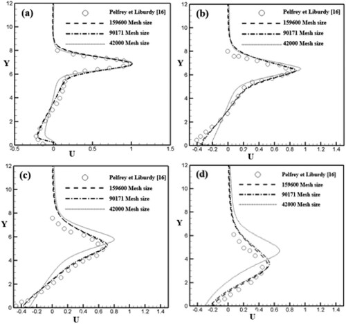
In Figure 4, the $U$ velocity profile at various axial locations i.e. X = 3, 6, 9 and 12 in Figure 4(a–d), respectively, are compared with experimental results of Pelfray and Liburdy [16] for an offset jet with OR = 6.5. In the same plots, three different meshes with 42,000, 90,171 and 159,600 number of cells are considered to perform the grid independence test. As noticed in Figure 4, the $U$ velocity profiles corresponding to number of (mesh) cells 90,171 and 159,600 almost overlap with each other and exhibit also a close match with the experimental data of Pelfray and Liburdy [16]. However, a significant difference is found when number of cells is increased from 42,000–90,171. Therefore, number of cells with 90,171 quadratic cells is considered for the remainder of computations.

Figure 4. Grid independence test and validation of computational results: axial velocity profiles at different axial locations (a) X = 3, (b) X = 6, (c) X = 9 and (d) X = 12.

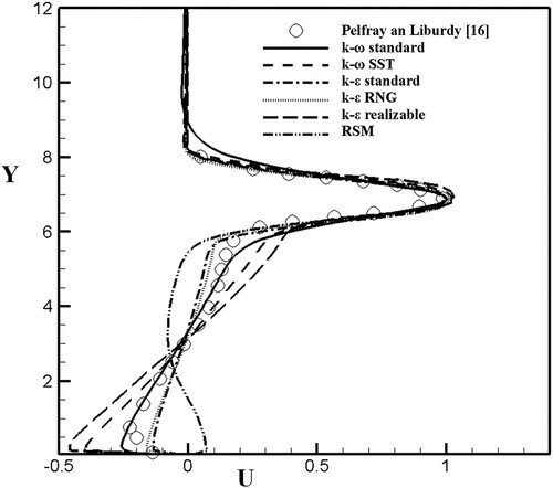
To justify the selection of the Wilcox k-ω model for the present numerical simulation, the U velocity profile at the axial location X = 3 is plotted in Figure 5 for six different turbulence models (standard k-ε, RNG k-ε, realizable k-ε, Wilcox k-ω, SST k-ω and Reynold Stress Model (RSM)) for number of cells 90,171 along with the corresponding experimental data of Pelfray and Liburdy [16]. It can be noticed in Figure 5 that numerical predictions match fairly well with those experimental of Pelfray and Liburdy [16] for the Wilcox k-ω model while some difference is observed for the other models. Therefore, for the rest of computations, the Wilcox k-ω model is used.

Figure 5. Turbulence model sensitivity test: axial velocity profiles at an axial location X = 3.

3. Results and discussion

3.1. Streamlines and mean velocity vectors

To demonstrate the flow pattern in the region close to the jets’ exit, the streamlines are plotted. Flow patterns in the recirculation region are visualized by streamlines in Figure 6(a–c) for co-flow velocity CFV = 0%, 20% and 40%, respectively, and a fixed offset ratio OR = 7. As expected, all recirculation zones in Figure 6 contain two primary vortices positioned one above the other: the clockwise rotating upper vortex is formed on the offset jet side, while the clockwise rotating lower vortex is formed on the wall jet side. Locations of upper and lower vortex centres are highlighted for each plot in Figure 6. At the vortex centre both the streamwise and the transverse velocities are zero. For the dual jet with OR = 7, the upper vortex centres (abbreviated as UVC) are found at $(X_{UVC},Y_{UVC})$: (3.60, 5.03), (3.86, 5.18), (4.01, 5.34) and the lower vortex centres (abbreviated as LVC) are found at $(X_{LVC},Y_{LVC})$: (3, 2.08), (3.28, 2.12), (3.58, 2.17), for CFV = 0%, 20% and 40%, respectively. These results suggest that the centres of both the vortices in the recirculation zone shift in the downstream as well as in the transverse direction as the magnitude of the co-flow velocity is increased.

Figure 6. Streamline pattern for offset ratio OR = 7 with different co-flow velocities: (a) CFV = 0%, (b) CFV = 20% and (c) CFV = 40%.

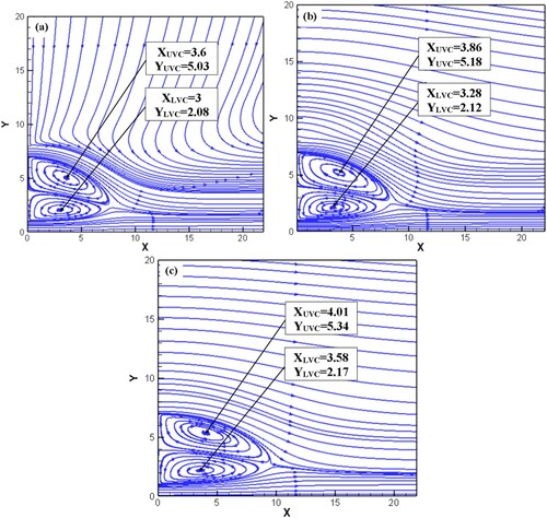
Figure 6 exhibits notable finite co-flow velocity effects. The direction of streamlines above the offset jet region for CFV = 0% in Figure 6(a) is directed almost vertically downwards due to the entrainment of neighbouring fluid towards the jets. However, for CFV = 20% and 40% in Figure 6(b,c), respectively, the streamlines above the offset jet are almost horizontal with a slight bend towards the bottom wall similar to the streamline pattern in case of flow past a 2D bluff body (e.g. [35]). In this case, the nozzle plate between the two jets acts as a 2D bluff body. Additionally, a close look on all the streamline plots in Figure 6 suggest that for CFV = 0% in Figure 6(a), the size of the upper vortex is relatively greater than that of the lower vortex due to the unequal entrainment of surrounding fluid by the two jets; the upper offset jet entrains more fluid than the lower wall jet owing to the presence of the bottom wall. However, with the increase of co-flow velocity to CFV = 40% in Figure 6(c), the two vortices are found to be almost equal in size, implying that the impact of the bottom wall on the recirculation bubble diminishes as the velocity of the co-flow is increased.

Mean velocity vectors are plotted to visualize the downstream development of the dual jet flow. Figure 7(a–c) shows the velocity vector of the mean flow with offset ratio OR = 7 for co-flow velocity CFV = 0%, 20% and 40%, respectively. Each flow region (i.e. converging, merging and combined regions) is distinctly evident from each of the vector plots. The negative velocity close to the nozzle exit indicates the flow reversal owing to the existence of a recirculation region. The merge (MP) and combined (CP) points are shown in all the velocity vector plots. At the merge point, the mean streamwise velocity remains to be zero (i.e. U = 0). The combined point corresponds to a point at which the two velocity peaks disappear to become a single peak and the mean streamwise velocity reaches to a maximum value.

Figure 7. Mean velocity vectors for OR = 7 with different co-flow velocities: (a) CFV = 0%, (b) CFV = 20% and (c) CFV = 40%.

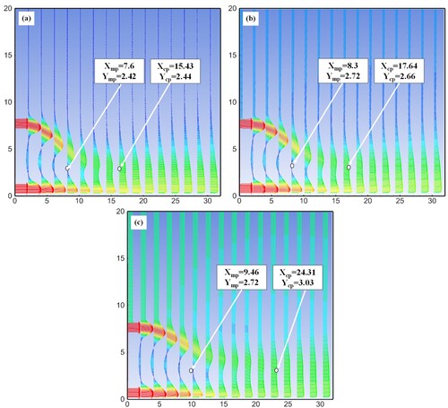
The mean velocity vectors in the outer part of the outer shear layer of the offset jet in Figure 7(a) attain the free-stream velocity since the flow is quiescent in this region. However, in the same region, the magnitude of the velocity vectors is comparable with the co-flow velocity as depicted in Figure 7(b,c) for CFV = 20% and 40%, respectively. The axial and the transverse locations of the merge point $(X_{mp},Y_{mp})$ and the combined point $(X_{cp},Y_{cp})$ are obtained at (7.6, 2.42), (8.3, 2.53), (9.46, 2.72) and (15.43, 2.44), (17.64, 2.66), (24.31, 3.03) for co-flow velocity CFV = 0%, 20% and 40%, respectively. The computed value of $X_{mp}$ for CFV = 0% (i.e.$X_{mp}=7.60$) is in reasonable agreement with $X_{mp}=8.41$ from Kumar [30] for a dual jet with OR = 7 and $X_{mp}=7.42$ from Spall et al. [36] for two parallel jets with OR = 7. The combined points are found to be at an axial distance $X_{cp}=15.43$, 17.64 and 24.31 for CFV = 0%, 20% and 40%, respectively. In comparison, the combined length is found to be 16.85 in Kumar [30] for the dual jet flow with OR = 7, $X_{cp}=18.22$ for the standard $k-\epsilon$ model and 18.34 for the RSM model in Anderson and Spall [37] for two parallel jets with offset ratio OR = 9.

3.2. Contour of ($\mathbf{\text{U}}=0$, $\mathbf{\text{V}}=0$) and $\frac{\mathrm{\partial }\mathbf{\text{U}}}{\mathrm{\partial }\mathbf{\text{Y}}}=0$

In order to accurately capture the locations of MP, UVC and LVC, the combined contours of $\text{U}=0$ and $\text{ V}=0$ are plotted and for CP, only the contour of $\frac{\mathrm{\partial }\text{U}}{\mathrm{\partial }\text{Y}}=0$ is plotted. Figure 8(a–d) display the contours of $\text{U}=0$ and $\text{ V}=0$ together in the near field region for offset ratio OR = 5, 7, 9 and 11, respectively. Since, by definition, both U and V velocities at the merge point and at the vortex centre are zero, the intersection of the contour lines U = 0 and V = 0 represents the locations of MP, UVC and LVC. The solid lines in Figure 8, represent the contours of U = 0, while the dashed lines in the same plot represent the contours of V = 0. For clarity of the presented results, a zoomed view for UVC and LVC positions is shown beside each plot in Figure 8.

Figure 8. Contours of U = 0, V = 0 for different offset ratios: (a) OR = 5, (b) OR = 7, (c) OR = 9 and (d) OR = 11.

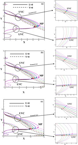
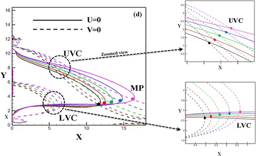
It is clearly visible from Figure 8 that, for a given offset ratio, with the progressive increase of co-flow velocity, the flow characteristic points in the converging region i.e. MP, UVC and LVC gradually shift towards the further downstream locations in the flow field with a trend of slowly moving in the transverse direction. This fact indicates that the co-flow stream has an influence on the converging region of the dual jet flow. Additionally, Figure 8 indicates that as the offset ratio increases, for a given co-flow velocity, all these characteristic points in the converging region relocate themselves towards the further downstream direction of the dual jet flow field with an increased height above the bottom wall. This is quite obvious in a sense that as the offset height increases, the size of the recirculation region also increases; thus, the merge point shifts its location in the further downstream direction.

The combined point (CP) is characterized by a location in the flow domain where the two jets combine with each other to become an equivalent single jet. Therefore, the two peaks in the velocity profile downstream of the merge point vanish to become a single peak at the combined point. In terms of the mathematical expression, the gradient of streamwise velocity component with respect to the transverse direction at the combined point is zero i.e. $\frac{\mathrm{\partial }\text{U}}{\mathrm{\partial }\text{Y}}=0$ at CP. The same concept is implemented in the present study to identify the location of the combined point in the flow domain. Figure 9 shows the contours of $\frac{\mathrm{\partial }\text{U}}{\mathrm{\partial }\text{Y}}=0$ for offset ratios OR = 5, 7, 9 and 11, respectively, at different values of co-flow velocity within the range CFV = 0%–40%. As per the definition of the combined point mentioned above, the vertex of the contour line $\frac{\mathrm{\partial }\text{U}}{\mathrm{\partial }\text{Y}}=0$ represents the combined point CP in all the plots in Figure 9.

Figure 9. Contours of dU/dY = 0 for different offset ratios: (a) OR = 5, (b) OR = 7, (c) OR = 9 and (d) OR = 11.

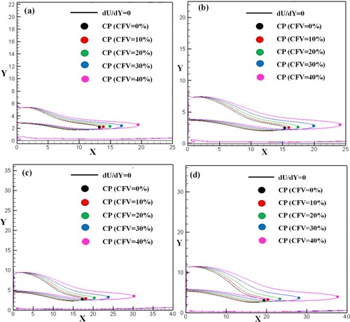
As shown in Figure 9, for a fixed value of OR, like the other characteristic points (i.e. MP, UVC and LVC), the combined point CP is found to occur in further downstream direction together with an upward displacement of CP towards the co-flow side with an increase in the co-flow velocity. Since the momentum of the co-flow in the streamwise direction increases with increasing the CFV, the deflection of the offset jet towards the co-flow side is found to be more pronounced for the higher co-flow velocity. Thus, both the streamwise distance of CP from the jet exit and the transverse distance of CP from the horizontal wall are found to increase with increasing the co-flow velocity. Furthermore, it is observed that the displacement of the combined point in the downstream direction is significantly greater than that in the transverse direction for a given offset ratio. For a given co-flow velocity, Figure 9 also shows that the location of the combined point from the jet exit plane increases invariably when the offset ratio is increased from OR = 5 to OR = 11. This is due to a stronger interaction between the two jets for the dual jet with a higher offset ratio.

3.3. Mean velocity profiles

To show the evolution of various shear layers in the flow domain, the profiles of the streamwise velocities are presented in Figure 10 at six selected locations in the further axial direction (two stations in each region) in the range $0\le \text{X}\le 30$ for various percentage values of co-flow velocities for a fixed offset ratio of the dual jet i.e. OR = 7. The axial locations are chosen such the locations are common in each region (converging, merging and combined regions).

Figure 10. Mean velocity profile at different axial locations: (a) X = 3, (b) X = 5, (c) X = 12, (d) X = 14, (e) X = 28, (e) and (f) X = 30.

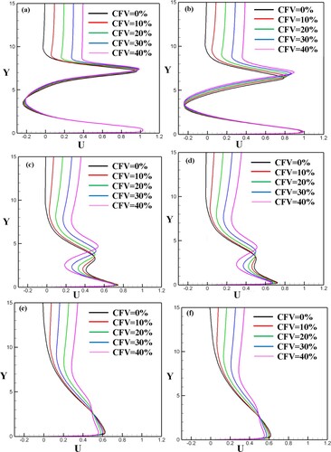
Two peaks (upper peak for offset jet while lower one for wall jet) distinctly appear in the velocity profile for all cases of CFV up to the axial distance X = 14 due to the existence of four shear layers: outer (layer 1) and inner (layer 2) shear layers for the offset jet, outer shear layer for the wall jet (layer 3) and wall boundary layer, as indicated in the schematic diagram in Figure 1.

At the outer side of the outer shear layer of the offset jet, the U velocity profile is vertically straight almost constant for CFV = 0% but it is a little bent for cases of finite CFV > 0 to assume the upstream flow conditions at the upper boundary. In the further vicinity of jet exit, at X = 3 and 5, the negative U velocity confirms the occurrence of a recirculation region in between the two jets. At X = 3, all the U velocity profiles almost overlap with each other up to the transverse distance Y = 8 (i.e. up to the layer 2); however, with increase of X, all the profiles gradually begin to deviate from each other.

From X = 14 onwards, the two U velocity peaks eventually vanish and only a single peak survives in the further downstream at X = 30 for each case of CFV except the case with CFV = 40%, indicating that the two jets for CFV = 40% are yet to combine together at this location which is evident from the velocity vector plot in Figure 7. All velocity profiles apart from CFV = 40% at X = 30 resemble a wall jet like flow.

It can be noticed from Figure 10 that the magnitude of the U velocity peak for the wall jet (between layer 3 and the wall boundary layer) at a given axial location is greater than that of the velocity peak for the offset jet (between layer 1 and layer 2) because of the higher exchange of momentum of the offset jet in the transverse direction. Also, both the peaks gradually decrease as the axial distance increases, where the offset jet peak decreases faster than the wall jet peak, implying that the combined flow is approaching to a flow structure like the wall jet. The transverse position of the U velocity peaks for the offset jet gradually disappears with the downstream distance, while that for the wall jet remains almost unaltered. This increase in co-flow velocity strongly restricts the offset jet deviating to the wall jet. These results are consistent with the results shown in Figure 8 for MP, UVC and LVC and Figure 9 for CP.

3.4. Decay of maximum streamwise velocity

To show the variation of centerline velocity of the jets, the maximum streamwise velocity $U_{\text{max}}$ is plotted given in Figure 11. The decay of $U_{\text{max}}$ for the offset jet is shown up to the combined point since the two jets merge to form a single jet. Figure 11 delineates the effects of co-flow velocity on the decay of maximum streamwise velocity for OR = 7. In the vicinity of the nozzle exit, $U_{\text{max}}$ is found to remain constant at $U_{\text{max}}$ up to a certain distance, indicating the existence of a potential core region. The potential core length varies insignificantly with the change in the percentage variation of co-flow velocity for either of the jets in the range CFV = 0%–40%. However, for a given value of CFV, the length of the potential core for the wall jet is found to be larger than that for the complementary offset jet, suggesting the spreading of offset jet is faster than that of the wall jet in dual jet flow.

Figure 11. Effect of co-flow velocity (CFV) on maximum axial velocity ($U_{\text{max}}$) decay for OR = 7.

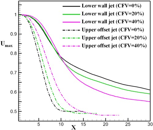
After the potential core region, $U_{\text{max}}$ for the wall jet decays monotonically from the nozzle towards the combined point, while the same flow quantity for the offset jet decays sharply up to some downstream distance followed by an asymptotic decay to attain a constant value at the combined point. This decay of $U_{\text{max}}$ is fastest for CFV = 0% and slowest for CFV 40%. This can be attributed to the resisting shear stress imposed on the outer shear layer of the offset jet is less for the dual jet with higher CFV. In the merging region, the decay of $U_{\text{max}}$ in offset jet is seen faster than that in wall jet at a given value of CFV. This is evident in velocity vector plot as well in Figure 7(b), implying the growth of the shear layer is greater for the offset jet than that for the wall jet due to the higher entrainment of fluid in the case of the offset jet. The co-flow velocity in fact does not appreciably affect the maximum streamwise velocity for the lower wall jet in the converging region because the wall remains intact from the effects of the co-flow before the merge point (MP). In the combined region, although the rate of decay of $U_{\text{max}}$ is almost the same for all the cases of dual jet flows investigated similar to the case of a classical wall jet, the value of $U_{\text{max}}$ remains greater for the lower CFV dual jet.

3.5. Wall pressure and friction coefficients

The wall pressure and skin friction coefficients help to identify different regimes in the flow domain of the dual jet. Figures 12(a,b) represent the distribution of the wall pressure coefficient $C_p=\frac{p_w-p_a}{0.5\times \rho \times u_0^2}$ ($p_w$ and $p_a$ are the wall and ambient pressures, respectively) and skin friction coefficient $C_f=\frac{{\tau }_w}{0.5\times \rho \times u_0^2}$, respectively, for various co-flow velocities in the range CFV = 0%–40% and offset ratio OR = 7. The effect of co-flow velocity variation is vividly noticed due to the exhibition of highest and lowest values of the wall pressure coefficient $C_p$ along the wall in Figure 12(a). For a fixed CFV, the wall pressure decreases to a minimum value (sub-atmospheric) immediate downstream of the nozzle exit followed by a recovery of pressure to a value above the atmospheric one to reach a maximum value before it gradually decreases in the merging region. For all the cases of CFV, the $C_p$ peak occurs close to the streamwise distance of the merge point $(X_{mp})$.

Figure 12. Effect of the co-flow velocity (CFV) on the pressure (a) and friction (b) coefficients.

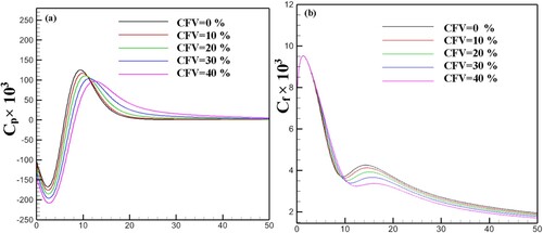
In the far downstream region, the pressure remains almost constant, signifying a flow structure resembling a classical wall jet. The peak value of wall pressure is noticed to be maximum for CFV = 0% and minimum for CFV = 40%. This occurrence of lower wall pressure confirms that in the converging region the co-flow stream hinders the offset jet more strongly to merge with the wall jet. Owing to this, the merge point is located closer to the wall for the lower values of the co-flow velocity. In the merging region, the wall pressure gradually decreases with the axial distance, an indication of the acceleration of the flow owing to the merging of two jets. In this region, the rate of decay of the wall pressure fastest for CFV = 0% and slowest for CFV = 40%.

The flow acceleration in the merging region is obstructed by the co-flow stream above the offset jet and thus the flow acceleration decreases as the velocity of the co-flow stream is increased. Although the distribution curves remain identical, the values of highest and lowest peaks of the wall pressure are different for different percentage values of the co-flow velocities. It can also be seen from Figure 12(a) that the progressive change in the co-flow velocity not only changes the peak value of $C_p$ but also causes an axial displacement of the peak position. This indeed indicates a gradual enlargement of the recirculation bubble in between the two jets with the progressive increase of the co-flow velocity.

The skin friction coefficient measures the wall shear stress in units of the stagnation pressure. The effects of co-flow velocity on the variation of $C_f$ is illustrated in Figure 12(b) for a dual jet with offset ratio OR = 7. For all cases of CFV, $C_f$ attains a maximum value near the nozzle exit before sharply decreasing in the rest of the converging region. The effects of co-flow velocity on skin friction in the converging region are negligible as all the profiles almost overlap with each other in this region. This is quite obvious because in this region, the wall jet remains unaffected by the offset jet.

In the merging region, the skin friction coefficient shows a peak due to the acceleration of flow after the merge point followed by a monotonic decrease along the X distance due to frictional drag. Although the influence of the co-flow velocity is quite prominent in the merging region, it eventually diminishes with the axial distance. In the merging region, Figure 12(b) shows that the peak value of $C_f$ is highest for CFV = 0% (i.e. no upstream flow) and lowest for CFV = 40%. In other words, the lower is the co-flow velocity, the higher is the wall shear stress. The reason can be given as follows: as the strength of the co-flow velocity decreases, the offset jet inclines more towards the wall jet and the merged flow stays closer to the bottom wall, causing higher wall shear stresses for lower values of the co-flow velocity.

3.6. Locations of flow characteristic points

To visualize the effects of co-flow velocity on the locations of flow characteristic points, Figure 13(a–d) and Figure 14(a–d) are plotted for the axial and transverse locations of MP$(X_{mp},Y_{mp})$, CP$(X_{cp},Y_{cp})$, UVC $(X_{uvc},Y_{uvc})$ and LVC$(X_{lvc},Y_{lvc})$, respectively, for co-flow velocity in the range CFV = 0%–40% and offset ratio in the range OR = 5–11. Numerical results are presented with symbols and those extracted from correlations with lines. The correlations functions will be discussed in the next section. Table 2 shows the values of axial and transverse locations of MP, CP, UVC and LVC for the range of CFV = 0%–40% and OR = 5–11 investigated. The same data are plotted in Figures 13 and 14.

Figure 13. Axial locations of the MP, CP, UVC and LVC: comparison between correlations and numerical results.

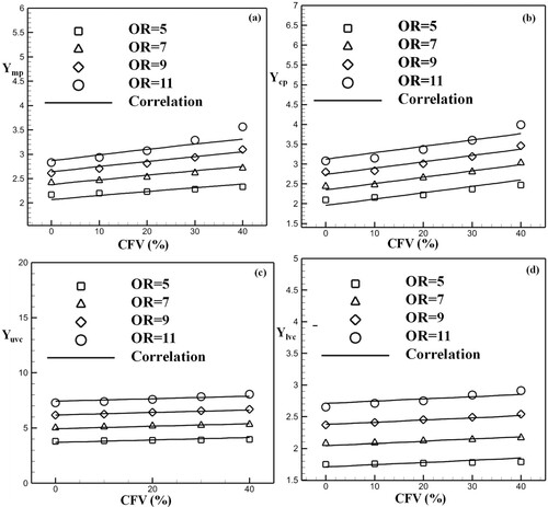
Figure 14. Lateral locations of the MP, CP, UVC and LVC: comparison between correlations and numerical results.

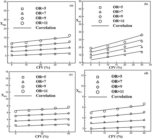
Table 2. Axial and lateral location of the MP, CP, UVC and LVC for different values of OR and CFV.

Merge point (MP)
OR		5		7		9		11
X and Y Locations	X	Y	X	Y	X	Y	X	Y
CFV (%)	0	5.28	2.17	7.6	2.42	9.69	2.61	11.65	2.83
	10	5.49	2.20	7.88	2.45	10.12	2.70	12.25	2.93
	20	5.67	2.23	8.3	2.53	10.81	2.81	13.26	3.04
	30	5.92	2.28	8.82	2.61	11.73	2.92	14.62	3.28
	40	6.16	2.33	9.46	2.72	12.83	3.10	16.28	3.56
Combined point (CP)
CFV (%)	0	13.38	2.10	15.43	2.44	17.43	2.80	19.42	3.08
	10	13.90	2,16	16.05	2.48	18.28	2.83	20.51	3.15
	20	15.11	2,22	17.64	2.66	20.38	3.01	23.30	3.37
	30	16.89	2,37	20.14	2.81	23.86	3.19	28.04	3.60
	40	19.50	2,47	24.31	3.03	30.28	3.46	37.68	3.99
Upper Vortex Centre (UVC)
CFV (%)	0	2.28	3.80	3.60	5.03	5.00	6.15	6.30	7.28
	10	2.33	3.86	3.75	5.11	5.22	6.25	6.61	7.40
	20	2.35	3.89	3.86	5.18	5.43	6.40	6.96	7.59
	30	2.39	3.92	3.93	5.25	5.62	6.55	7.32	7.82
	40	2.40	3.95	4.01	5.34	5.81	6.70	7.61	8.06
Lower Vortex Centre (LVC)
CFV (%)	0	1.98	1.75	3.00	2.08	4.00	2.37	4.91	2.65
	10	2.05	1.76	3.15	2.09	4.21	2.41	5.24	2.71
	20	2.09	1.77	3.28	2.12	4.47	2.45	5.66	2.75
	30	2.16	1.78	3.43	2.14	4.76	2.49	6.14	2.84
	40	2.20	1.79	3.58	2.17	5.06	2.54	6.62	2.91

As noticed from Figures 13 and 14, for a given offset ratio, the trend of variations for both the axial and transverse locations of MP, CP, UVC and LVC remains almost identical. However, for a given CFV, as expected, the values of both X and Y locations for all the characteristic points increase with the increase of the offset ratio from 5 to 11. For a fixed value of the offset ratio, the values of $X_{mp},X_{cp}$ in Figure 13 and $Y_{mp},Y_{cp}$ in Figure 14 keep increasing with the co-flow velocity CFV, which can be discerned in the contour plots shown in Figures 8 and 9, respectively. This result confirms that the increase in co-flow velocity leads to a further displacement of MP and CP to the downstream direction with a gradual shift away from the bottom wall in a positive Y direction.

Although the data points for some cases of the characteristic points in Figures 13 and 14 indicate a non-linear variation, all the correlation curves exhibit a linear trend with the co-flow velocity for a given value of the offset ratio. The variations of correlation curves for $X_{uvc}$ and $X_{lvc}$ in Figure 13 and $Y_{uvc}$ and $Y_{lvc}$ in Figure 14 remain almost constant, indicating a negligible influence of the co-flow velocity on the recirculation region of the dual jet flow. For a given OR, the slope of the correlation curves for both MP and CP remains higher than that for UVC and LVC. Although the slope of correlation curves for $Y_{mp}$ vs. CFV in Figure 14(a) and $Y_{cp}$ vs. CFV in Figure 14(b) remains almost same, the same for $X_{cp}$ vs. CFV in Figure 13(b) is found to be greater than that for $X_{mp}$ vs. CFV in Figure 13(a). The trend of correlations curves for all the characteristic points suggests that the influence of co-flow velocity in the merging region is greater than that in the converging region.

3.7. Correlation functions

For a quick estimation of the positions of characteristic points at a given co-flow velocity and an offset ratio for a dual jet flow, various correlation functions are derived for the locations of MP, CP, UVC and LVC with respect to combined CFV and OR. For this purpose, a linear regression analysis is performed on both the axial and transverse locations for each of the flow characteristic points. The empirical correlations obtained from the regression analysis for $X_{\text{MP}},X_{\text{CP}},X_{\text{UVC}}$ and $X_{\text{LVC}}$ are expressed in terms of combined CFV and OR in Equations 6–9, respectively, for CFV = 0%–40% and OR = 5–11. (6) $\begin{array}{rl}{X}_{\text{MP}}& =e^{-3.53106}\times \text{O}{\text{R}}^{1.0965127}\times (\text{CFV}+100{)}^{0.73492}\end{array}$(6) (7) $\begin{array}{rl}{X}_{\text{CP}}& =e^{-5.36122}\times \text{O}{\text{R}}^{0.59512}\times (\text{CFV}+100{)}^{1.49301}\end{array}$(7) (8) $\begin{array}{rl}{X}_{\text{UVC}}& =-1.8599+0.7708\times \text{OR}+0.016625\times \text{CFV}\end{array}$(8) (9) $\begin{array}{rl}{X}_{\text{LVC}}& =e^{-4.2}\times \text{O}{\text{R}}^{1.26742}\times (\text{CFV}+100{)}^{0.60855}\end{array}$(9)

The curves based on these empirical formulae are plotted in Figure 13(a–d) along with the corresponding curves data points obtained numerically for $X_{\text{MP}},X_{\text{CP}},X_{\text{UVC}}$ and $X_{\text{LVC}}$, respectively. As indicated in Figure 13, the proposed correlation functions exhibit a fairly good agreement with the corresponding computational results with an overall accuracy of 96.4%, 94.9%, 97.1% and 98.1% for $X_{\text{MP}},X_{\text{CP}},X_{\text{UVC}}$ and $X_{\text{LVC}}$, respectively. The overall accuracy is obtained by taking the average of percentage deviation of the correlation data with respect to the numerical data of the characteristic point for the entire range of offset ratio considered. It can be remarked here that except $X_{\text{UVC}}$, the axial locations for all other cases (i.e. $X_{\text{MP}},X_{\text{CP}},X_{\text{UVC}}$ and $X_{\text{LVC}}$), the combined correlation functions hold a power-law relationship with both CFV and OR. The axial location for the upper vortex centre $X_{\text{UVC}}$, on the other hand, shows only a linear relationship.

The regression analysis is also performed for the transverse locations of MP, CP, UVC and LVC. The correlations functions obtained as an outcome of the regression analysis are presented in Equations (10–13) for $Y_{\text{MP}},Y_{\text{CP}},Y_{\text{UVC}}$ and $Y_{\text{LVC}}$, respectively. The transverse coordinate of MP, CP, UVC and LVC are plotted in Figure 14 along with the corresponding numerical results. The correlation curves fit well with the corresponding computational results with an accuracy of97.2%, 97.6%, 98.9% and 99% for $Y_{\text{MP}},Y_{\text{CP}},Y_{\text{UVC}}$ and $Y_{\text{LVC}}$, respectively. Similar to $X_{\text{MP}}$, $Y_{\text{MP}}$ also holds a power-law relationship jointly with CFV and OR. However, the transverse locations for other flow characteristic point are the linear function of combined CFV and OR. (10) $\begin{array}{rl}{Y}_{\text{MP}}& =e^{-1.93656}\times \text{O}{\text{R}}^{0.4152}\times (\text{CFV}+100{)}^{0.4329}\end{array}$(10) (11) $\begin{array}{rl}{Y}_{\text{CP}}& =0.9821+0.016025\times \text{OR}+0.1948\times \text{CFV}\end{array}$(11) (12) $\begin{array}{rl}{Y}_{\text{UVC}}& =0.5651+0.6233\times \text{OR}+0.01125\times \text{CFV}\end{array}$(12) (13) $\begin{array}{rl}{Y}_{\text{LVC}}& =0.8733+0.1669\times \text{OR}+0.0035\times \text{CFV}\end{array}$(13)

4. Conclusions

The present work involving a numerical investigation on a dual jet (coupled wall and offset jets) accompanied by a co-flow stream parallel to the jets’ centrelines is solved. The flow arrangement configuration of a dual jet is often observed in sewage disposal systems. By varying the velocity of the co-flow and the offset ratio separately, the emission of the wastewater into the rivers, seas and oceans may be controlled. This plays a significant role for the motivation of the present study.

A CFD package “ANSYS FLUENT” is used for purpose of computation conducting the numerical simulations. The Wilcox k-ω model is used for predicting the turbulent flow. The Reynolds number (based on the reference velocity u₀ and jet width w) considered for the present is 15,000. The numerical predictions are obtained to are primarily examined with respect to the effects of co-flow on the $(X,Y)$ positions of the various characteristic points in the flow field i.e. merge point (MP), combined point (CP), upper vortex centre (UVC) and lower vortex centre (LVC). A key result of the present study is simple correlations between the location of each characteristic point in terms of the combined co-flow velocity (CFV) and the offset ratio (OR, which is defined here as the height of the offset jet nozzle from the bottom wall per unit jet width). For this purpose, both the co-flow velocity and the offset ratio are varied in a wide range: the co-flow velocity is varied in the range CFV = 0%–40% (where CFV is the ratio of co-flow velocity to the jet velocity), and the offset ratio is varied within the range OR = 5–11.

The mean flow field contains a recirculation region between the two jets consisting of two vortices located one above the other. For the investigated case without co-flow velocity, the size of the upper vortex remains always larger than that of the lower one. However, this difference in size gradually diminishes with the increase of co-flow velocity and thus for a higher value of co-flow velocity, so that these two vortices become almost equal to each other. With the increase of co-flow velocity, all the characteristic points i.e. MP, CP, UVC and LVC shift both in axial and transverse direction. This shift in the downstream direction is found to be larger than that in the transverse direction.

The rate at which the maximum mean streamwise velocity $U_{\text{max}}$ decays in the downstream direction is faster for the offset jet and this decay rate is fastest for CFV = 0% and slowest for CFV = 40% in case of the offset jet. Although the variation of $U_{\text{max}}$ in case of the wall jet is seen to be more or less the same up to the merging region for different co-flow velocities, in the combined region, the rate of decay of $U_{\text{max}}$ is fastest for CFV = 40% and slowest for CFV = 0%. The variation of the pressure coefficient $(C_p)$ along the bottom wall exhibits a single peak just downstream of the merging point and the value of this peak is found to be maximum for CFV = 0% and minimum for CFV = 40%. As the co-flow velocity increases, the peak position for $C_p$ is gradually relocated along the downstream direction. No change in the profile of the skin friction co-efficient $(C_f)$ on the bottom wall is detected in the converging region with the increase of the co-flow velocity. However, an appreciable amount of variation in $C_f$ is seen in the merging region for the peak which is highest for CFV = 0% and lowest for CFV = 40%.

For a given offset ratio, the trends of variation for various characteristic points in both downstream and transverse directions with respect to the co-flow velocity are found to be identical; however, the co-flow stream has a strong influence on the merge point as well as on the combined point compared to the position of the two vortex centres and this influence increases with increasing the co-flow velocity. Interestingly, for OR = 5, the effect of the co-flow stream on the recirculation region is seen almost virtually. The empirical correlation holds a combined power-law relationship of $X_{mp},Y_{mp},X_{cp}$ and $X_{lvc}$ with CFV and OR, while $Y_{cp},X_{uvc},Y_{uvc}$ and $Y_{lvc}$ are found to vary linearly with both CFV and OR. The computational results reveal that the wall jet remains more or less intact with the variation of either CFV or OR, but the offset jet is affected considerably by these two parameters.

Disclosure statement

No potential conflict of interest was reported by the author(s).

Additional information

Funding

This research has been funded by Scientific Research Deanship at University of Ha’il – Saudi Arabia through project number [grant number RG-21 034].

References

- Forthmann E. (1936). Turbulent jet expansion. National Advisory Committee for Aeronautics, Technical Memorandum no. 789, Washington, DC.
- Myers GE, Schauer JJ, Eustis RH. Plane turbulent wall jet flow development and friction factor. Trans ASME J Basic Eng. 1963;85(1):47–53.
- Gutmark E, Wygnanski I. The planar turbulent jet. J Fluid Mech. 1976;73(3):465–495.
- Launder BE, Rodi W. The turbulent wall jet. Prog Aerosp Sci. 1981;19:81–128.
- Abrahamsson H, Johansson B, Lofdahl L. The turbulent plane two dimensional wall-jet in a quiescent surrounding. Eur J Mech B/Fluids. 1994;13(5):533–556.
- Schneider M, Goldstein RJ. Laser Doppler measurement of turbulence parameters in a two-dimensional plane wall jet. Phys Fluids. 1994;6(9):3116–3129.
- Eriksson JG, Karlsson RI, Persson J. An experimental study of a two-dimensional plane turbulent wall jet. Exp Fluids. 1998;25(1):50–60.
- George WK, Abrahamsson H, Eriksson J, et al. A similarity theory for the turbulent plane wall jet without external stream. J Fluid Mech. 2000;425:367–411.
- Dejoan A, Leschziner MA. Large eddy simulation of a plane turbulent wall jet. Phys Fluids. 2005;17(2):025102(1–16).
- Ahlman D, Brethouwer G, Johansson AV. Direct numerical simulation of a plane turbulent wall-jet including scaler mixing. Phys Fluids. 2007;19:065102–1–13.
- Azim M. On the structure of a plane turbulent wall jet. Trans ASME J Fluids Eng. 2013;135:084502–1–4.
- Wei T, Wang Y, Yang XIA. Layered structure of turbulent plane wall jet. Int J Heat Fluid Flow. 2021;92:108872-1-11
- Bourque C, Newman BG. Reattachment of a two-dimensional incompressible jet to an adjacent flat plate. Aeronaut Quart. 1960;11:201–232.
- Sawyer RA. The flow due to a two-dimensional jet issuing parallel to a flat plate. J Fluid Mech. 1960;9(4):543–559.
- Sawyer RA. Two-dimensional reattachment jet flows including the effect of curvature on entrainment. J Fluid Mech. 1963;17(4):481–498.
- Pelfrey JRR, Liburdy JA. Effect of curvature on the turbulence of a two-dimensional jet. Exp Fluids. 1986a;4(3):143–149.
- Pelfrey JRR, Liburdy JA. Mean flow characteristics of a turbulent offset jet. Trans ASME J Fluids Eng. 1986b;108(1):82–88.
- Koo HM, Park SO. Prediction of turbulent offset jet flows with an assessment of QUICKER scheme. Int J Numer Methods Fluids. 1992;15(3):355–372.
- Gu R. Modelling two-dimensional turbulent offset jets. J Hydraul Eng. 1996;122(11):617–624.
- Kim DS, Yoon SH, Lee DH, et al. Flow and heat transfer measurements of a wall attaching offset jet. Int J Heat Mass Transfer. 1996;39:2907–2914.
- Gao N, Ewing D. Experimental investigation of planar offset attaching jets with small offset distances. Exp Fluids. 2007;42(6):941–954.
- Rathore SK, Das MK. Comparison of two low-Reynolds number turbulence models for fluid flow study of wall bounded jets. Int J Heat Mass Transfer. 2013;61:365–380.
- Singh TP, Kumar A, Satapathy AK. Fluid flow analysis of a turbulent offset jet impinging on a wavy wall surface. Proc IME C J Mech Eng Sci. 2019;234(2):544–563.
- Wang XK, Tan SK. Experimental investigation of the interaction between a plane wall jet and a parallel offset jet. Exp Fluids. 2007;42:551–562.
- Kumar A, Das MK. Study of a turbulent dual jet consisting of a wall and an offset jet. Trans ASME J Fluids Eng. 2011;133(10):101201.
- Li Z, Huai W, Han J. Large eddy simulation of the interaction between wall jet and offset jet. J Hydrodyn. 2011;23(5):544–553.
- Mondal T, Das MK, Guha A. Numerical investigation of steady and periodically unsteady flow for various separation distance between a wall and an offset jet. J Fluids Struct. 2014;50:528–546.
- Mondal T, Das MK, Guha A. Transition of a steady to a periodically unsteady flow for various Jet widths of a combined wall jet and offset jet. Trans ASME J Fluid Eng. 2016;137:071206.
- Mondal T, Guha A, Das MK. Computational study of periodically unsteady interaction between a wall jet and offset jet for various velocity ratio. Comput Fluids. 2015;123:146–161.
- Kumar A. Mean flow characteristics of a turbulent dual jet consisting of a plane wall jet and a parallel offset jet. Comput Fluids. 2015;114:48–65.
- Hnaien N, Marzouk S, Ben Aissia H, et al. Numerical investigation of velocity ratio effect in combined wall and offset jet flows. J Hydrodyn. 2018;30(6):1105–1119.
- Hnaien N, Marzouk S, Kolsi L, et al. Offset jet ejection angle effect in combined wall and offset jets flow: numerical investigation and engineering correlations. J Braz Soc Mech Sci Eng. 2019;41(11):478–495.
- Assoudi A, Mahjoub Saïd N, Bournot H, et al. Comparative study of flow characteristics of a single offset jet and a turbulent dual jet. Heat Mass Transfer. 2019;55(4):1109–1131.
- Ayech SBH, Habli S, Saïd NM, et al. A numerical study of a plane turbulent wall jet in a coflow stream. J Hydro-Environ Res. 2016;12:16–30.
- Chang YS, Chen YJ, Qiu YH, et al. Source-like patterns of flow past a circular cylinder of finite span at low Reynolds numbers. Phys Fluids. 2021;33(8):083607 .
- Spall RE, Anderson EA, Allen J. Momentum flux in plane, parallel jets. Trans ASME J Fluids Eng. 2004;126(4):665–670.
- Anderson EA, Spall RE. Experimental and numerical investigation of two-dimensional parallel jets. Trans ASME J Fluids Eng. 2001;123(2):401–406.