Bayesian analysis for geometric shapes in additive manufacturing

Abstract

In additive manufacturing, geometric shape deviations are built through statistical deviation models. Nonetheless, the resource constraints limit the manufacturers to test shapes. However, in addition to the power, the simplicity of the deviation models has been demonstrated with illustrative cases for in-plane deviation modelling for regular pentagon, irregular octagon as well as straight edges in free-form shapes utilizing only data and models for single regular pentagon and cylinders. Bayesian deviation models, built for geometric shapes, provide a better fit on the data and help in achieving better predictive accuracy. The main aim of this study is to assess the effect of the error distribution, generally assumed as the normal, and evaluate its impact on the deviation model. In particular, we consider Laplace, logistic, Cauchy, and exponential distributions for the errors. It is shown that logistic distribution provides better alternative error distribution for deviation models as compared to the normal distribution.

Keywords:

• Bayesian additive modelling
• geometric shapes
• deviations modelling
• cylinders
• regular pentagon
• irregular octagon

1. Introduction

Additive manufacturing (AM) is a mechanism which facilitates the direct production of complex geometric shapes [1, 2]. Three dimensional printing is a general term used to design and manufacture products with deep environmental, social, financial, and security implications. The benefits of AM include making complex geometries which may not be manufactured in any other way. As a result, new opportunities occur in designing industries, bio-engineering, automotive as well as aerospace. It is feasible with AM to make serviceable parts without the need of assembly to save time and cost of production [3, 4]. It decreases waste, minimizes the use of destructive chemicals and make possible the use of recycled materials [5].

Tong et al. [6, 7] used the observed deviation data to demonstrate the deviation of shapes in the Cartesian coordinates X, Y, and Z. In fact, the deviation data help in building a compensation strategy, amended shape through the computer-aided design (CAD) model with the objective that the altered form should have a close resemblance to the desired shape. To construct compensation plans, Huang et al. [8] presented a different functional modelling approach which justifies the relationship in dissimilar coordinates and separate geometric shape's complications from deviation modelling.

A general element of established quality control techniques for 3D printing is the application of deviation models for separate geometric shapes. These models, however, have a drawback, that is, tangible tests necessarily executed on numerous copies of each separate form to have an idea on their shape deviation models. To develop models, the resulting data are not successfully utilized and extensive utilization of these techniques is impracticable due to the very high operational costs of 3D printing that restrict the gathering data of deviation to a small sample of dissimilar shapes.

A challenge of in-plan shape deviation in 3D printing is the effective identification of new shape's deviation model by employing a small sample of formerly created dissimilar geometric shapes. Huang et al. [9] formulated a hypothesis in connection to a deviation model for irregular as well as regular polygons. A main restriction of the method, however, is the recognition of the functional shapes for different local deviation attributes which is principally heuristic. Huang et al. [9], however, could not define how an existed data library on geometric deviation may be utilized in order to study new deviation characteristics for new geometric shapes.

Sabbaghi et al. [10] introduced a model building technique for adaptive in-plane deviation models specified by Huang et al. [8] to account for a finite number of trial shapes. They suggested that the method makes use of some features of the deviation model for cylinder of Huang et al. [8] and the “cookie-cutter” deviation formulation suggested by Huang et al. [9].

Wang et al. [11] investigated the effect of process parameters on stereolithography (STL) part shrinkage. Sharon and Mumford [12] studied two-dimensional shape analysis by employing conformal mapping.

Huang et al. [9] discussed statistical predictive modelling as well as compensation of geometric shape deviations of three-dimensional manufactured goods. A predictive model is desired to forecast the value of an extensive class of product shapes, taking into consideration the vast library of AM built products with intricate geometry. They presented a unique statistical predictive modelling and compensation approach in order to have a better quality of cylindrical and prismatic parts. Both experimental exploration and validation of polyhedrons show that the methodology is promising for an extensive class of products constructed through 3D printing technology.

Huang et al. [8] discussed an ideal offline compensation plan of shape shrinkage for additive manufacturing procedures. They came up with a unique approach to (1) model and estimate part shrinkage and (2) draw an ideal shrinkage compensation plan in order to attain the accuracy of dimension. The expanded method is established experimentally as well as analytically in a stereolithography method, which is one of the most extensively used additive manufacturing methods. Jin et al. [13] proposed an off-line predictive control of out-of-plane shape deformation for 3D printing.

Huang et al. [14] described a logical basis for ideal compensation of 3D shape deformation in additive manufacturing. The study discussed an analytical basis to attain optimal compensation for high-precision additive manufacturing. Zhu et al. [15] discussed deviation modelling as well as shape alterations in design for the 3D printing. Systematic deviations are denoted by radial and polar coordinates and random deviations are modelled by translating the contour points with a specified distance which originates from the theory of random field.

Sabbaghi et al. [10] developed a Bayesian model from small samples of dissimilar data for obtaining in-plane deviation in 3D printing by using adaptive Bayesian modelling. Their approach successfully unites geometric shape deviation data and models for a minor sample of formerly developed, distinct geometric shapes to help in the model specification of geometric shape deviation for a wide category of novel forms. The procedure is illustrated for regular pentagon, irregular octagon and freestyle shapes with straight sides employing merely data and models for cylinders and a solitary regular five-sided polygon. We refer to [16–20] for some more recent literature on AM.

In Bayesian analysis, information concerning the unknown parameter of interest before the current data is known as the prior information. We, in this way, describe the prior distribution which is one's understanding or belief expressed by a probability distribution. With the possibility of the sample data, prior distribution is assimilated to derive a posterior distribution. Then, the posterior distribution is used for further inferences. Thus, the posterior belief is a mixture of prior belief and observed data which in future can be used as a prior information. The posterior predictive distribution (PPD) is the distribution for the future predicted data dependent on the observed data. The posterior predictive distribution is mainly utilized to predict values of new data. The posterior distribution is used to compute the predictive distribution, that is, averaging over the posterior distribution can help to predict uncertain prediction. Comparing the predictive distribution to observed data is generally named as the “posterior predictive check”. Unlike the frequentist statistics, this check comprises uncertainty related to the predicted parameters of the model. This is done by “simulating replicated data under the fitted model and then comparing these to the observed data” [21]. Hence, the posterior predictive will be used to “look for systematic discrepancies between the real and simulated data” [22].

The aim of this study is to evaluate the impact of random error distribution of deviation features for different shapes and suggest other appropriate distributions for different shapes. The choice of an appropriate prior has a significant impact on the Bayesian inference [23–28]. This work is an extension of Sabbaghi et al. [10], as they considered only the normal distribution for random errors of deviation features.

The rest of the study is organized as follows: Section 2 discusses the Bayesian model building for deviation features. Section 3 discusses the local and global Bayesian deviation model building for different geometric shapes like cylindrical, regular pentagon, irregular octagon, and free-form while Section 4 presents conclusion and recommendations.

2. Bayesian model building for deviation features

This section describes a basic characterization of deviation features along with the Bayesian model building taken from Sabbaghi et al. [10]. In particular, the modular deviation features for different shapes like cylinder, regular polygon, irregular polygon and free form are discussed [10].

2.1. Functional form of geometric shape deviation

Let thin 3D shapes with in-plane geometric shaped deviation with ignorable heights, as the main aim is to construct shape, that can be represented in two dimensions with identical top and surface deviations. To implement the deviational functional representation as outlined by Huang et al. [8], the (X, Y) Cartesian coordinates are translated into polar coordinates $\left(\vartheta ,\mathrm{{\rm Y}}\left(\vartheta \right)\right)$, with angle ϑ and radius $\mathrm{{\rm Y}}\left(\vartheta \right)$. Suppose ${\mathrm{{\rm Y}}}_s^{obs}\left(\vartheta \right)$ and ${\mathrm{{\rm Y}}}_s^{nom}\left(\vartheta \right)$ indicate the observed and nominal radius, respectively, of a shape s at $\vartheta \in [0,2\pi ]$. Every shape s related to a group of known parameters ${\gamma }_s$ describes the nominal radius form ${\mathrm{{\rm Y}}}_s^{nom}:\left[0,2\pi \right]\to \mathbb{R}$, with ${\gamma }_s$. Huang et al. [8] expressed the observed deviation at angle ϑ as (1) ${\mathrm{\nabla }}_s\left(\vartheta \right)={\mathrm{{\rm Y}}}_s^{obs}\left(\vartheta \right)-{\mathrm{{\rm Y}}}_s^{nom}\left(\vartheta \right)$(1)

2.2. Deviation models for different geometric shapes

Let two dissimilar shapes with nominal radius functions ${\mathrm{{\rm Y}}}_1^{nom}\left(\vartheta \right),{\mathrm{{\rm Y}}}_2^{nom}\left(\vartheta \right):\left[0,2\pi \right]\to \mathbb{R}$, respectively, where, ${\mathrm{{\rm Y}}}_1^{nom}(\cdot )$ parallel to earlier made shape for which model of deviation has been understood, and ${\mathrm{{\rm Y}}}_2^{nom}(\cdot )$ matches to one freshly made shape whose different features of deviation need to be revealed and formed. For ${\mathrm{{\rm Y}}}_1^{nom}(\cdot )$, assume the following deviation model [10]: (2) ${\mathrm{\nabla }}_1\left(\vartheta \right)={\delta }_1\left(\vartheta |\text{β}\right)+{\mathcal{E}}_1\left(\vartheta \right)$(2) where the systematic deviation is defined by the functional form ${\delta }_1\left(\vartheta |\text{β}\right)$, β is a vector of parameter, and ${\mathcal{E}}_1\left(\vartheta \right)$ are random errors with mean $E\left\{{\mathcal{E}}_1\left(\vartheta \right)\right\}=0$ at ϑ [8]. For instance, the function of ${\delta }_1$ can be written as $\begin{array}{rl}{\delta }_1\left(\vartheta |\text{β}\right)& =y_0+{\text{β}}_0{\left({\gamma }_1+y_0\right)}^{b_0}+{\text{β}}_1{\left({\gamma }_1+y_0\right)}^{b_1}\\ & \times \cos \left(2\vartheta \right)\end{array}$ where $\text{β}=({\text{β}}_0,{\text{β}}_1,b_0,b_1,y_0)$ [8]. The ${\mathrm{{\rm Y}}}_1^{nom}(\cdot )$ systematic deviation feature and ${\mathrm{{\rm Y}}}_2^{nom}(\cdot )$ deviation model are connected with each other through a local deviation feature ${\delta }_2\left(\vartheta |\alpha \right)$ [9, 29] (3) ${\mathrm{\nabla }}_2\left(\vartheta \right)={\delta }_1\left(\vartheta |\text{β}\right)+{\delta }_2\left(\vartheta |\alpha \right)+{\mathcal{E}}_2\left(\vartheta \right)$(3) Following this description, ${\delta }_1$ maintains the same global deviation aspect between ${\mathrm{{\rm Y}}}_1^{nom}(\cdot )$ and ${\mathrm{{\rm Y}}}_2^{nom}(\cdot )$, and ${\delta }_2$, with the parameter vector α, as a local deviation aspect matchless to the fresh shape [10]. The ${\mathcal{E}}_1\left(\vartheta \right)$ and ${\mathcal{E}}_2\left(\vartheta \right)$ are assumed identical and independent, with $E\left\{{\mathcal{E}}_2\left(\vartheta \right)\right\}=0$. The radius function for a regular n-sided polygon and circumcircle radius size $1^{″}$ are expressed as ${\mathrm{{\rm Y}}}_2^{nom}\left(\vartheta \right)=\frac{{\gamma }_1\cos \left(\frac{\pi }{n}\right)}{\cos \left\{\left(\vartheta -\frac{\pi }{2}\right)mod\frac{2\pi }{n}-\frac{\pi }{n}\right\}}$ where this function is clearly defined by the parameter vector ${\gamma }_2=\left(n,{\gamma }_1\right)$. Setting ${\mathrm{{\rm Y}}}_1^{nom}(\cdot )\equiv {\gamma }_1$ and utilizing ${\mathrm{{\rm Y}}}_2^{nom}(\cdot )$ in Equation (3(3) ${\mathrm{\nabla }}_2\left(\vartheta \right)={\delta }_1\left(\vartheta |\text{β}\right)+{\delta }_2\left(\vartheta |\alpha \right)+{\mathcal{E}}_2\left(\vartheta \right)$(3) ), a polygon deviation model can be obtained. Then, we can infer this specification of model by identifying theoretically, the carved polygon deviates globally in a same technique as its circumcircle. To distinguish ${\delta }_1$ for features like global deviation distributed among the polygon including circumcircle, the deviation of regular polygon varies from ${\delta }_1$ because of its sharp corners and straight sides, as it portrays the local deviation aspect. We take no additional assumptions about correlation between ${\delta }_1$ and ${\delta }_2$ [10].

The deviation model building for a new form ${\mathrm{{\rm Y}}}_2^{nom}(\cdot )$ can be summarized by identifying its local deviation aspect ${\delta }_2$ on freshly printed shape. Though such a heuristic local deviation model builds on pre-specified functions may not produce good approximation in an exercise as it is traditionally very hard to find a parsimonious priori and suitable local deviation conditions for complicated shapes. An alternative method which is very reasonable from a statistical viewpoint is to precisely understand that local deviation's qualities that continue across shapes build on a blend of prior assumptions for ${\delta }_1$ and observed deviation data for a freshly manufactured shape ${\mathrm{{\rm Y}}}_2^{nom}(\cdot )$.

2.3. An approach for modelling local deviation features

We consider the Bayesian model building methodology in three phases.

• Built a discrepancy measure [30, 31]) to isolate data on the feature of local deviation for a novel shape ${\mathrm{{\rm Y}}}_2^{nom}(\cdot )$.

• To explain the local deviation feature, block and cluster distributions of the discrepancy measure allowing covariates.

• Identify a model's hierarchy for the parameters α of the patterns over the blocks.

The first phase related to the construction of discrepancy measure can be achieved using Equation (3(3) ${\mathrm{\nabla }}_2\left(\vartheta \right)={\delta }_1\left(\vartheta |\text{β}\right)+{\delta }_2\left(\vartheta |\alpha \right)+{\mathcal{E}}_2\left(\vartheta \right)$(3) ). Suppose $D_1$ symbolizes the deviation data collection for produced shapes with the identical nominal radius function ${\mathrm{{\rm Y}}}_1^{nom}(\cdot )$ and $F\left(\text{β}|D_1\right)$ the posterior distribution of β build on $D_1$. The observed deviation data ${\mathrm{\nabla }}_2\left(\vartheta \right)$ is transformed for a novel produced shape into a random variable to express discrepancy measure as (4) $T_2\left(\vartheta \right)={\mathrm{\nabla }}_2\left(\vartheta \right)-{\delta }_1\left(\vartheta |\widetilde{\text{β}}\right)$(4) where $\widetilde{\text{β}}\sim F\left(\text{β}|D_1\right)$. The possible non-trivial global deviation feature can be efficiently eradicated by utilizing this transformation. A concrete and simple initial point to understand a function of ${\delta }_2$ in terms of ϑ and ${\mathrm{{\rm Y}}}_2^{nom}\left(\vartheta \right)$ is offered by this discrepancy measure and Monte Carlo simulations can be used to derive the distribution of this discrepancy measure appropriately. If ${\widetilde{\text{β}}}^l\sim F\left(\text{β}|D_1\right)$ for $l=1,\dots ,L$, then the distribution of the discrepancy measure given in Equation (4(4) $T_2\left(\vartheta \right)={\mathrm{\nabla }}_2\left(\vartheta \right)-{\delta }_1\left(\vartheta |\widetilde{\text{β}}\right)$(4) ) can be determined as (5) $T_2^{\left(l\right)}\left(\vartheta \right)={\mathrm{\nabla }}_2\left(\vartheta \right)-{\delta }_1\left(\vartheta |{\widetilde{\text{β}}}^{\left(l\right)}\right)$(5) Next, to obtain discrepancy measures into E blocks assuming covariates considered to be related to the feature of local deviation, each side will be a natural block for a polygon. To this end, categorize systematic patterns in $T_2\left(\vartheta \right)$ like a functional form of ϑ and ${\mathrm{{\rm Y}}}_2^{nom}\left(\vartheta \right)$ across and within the E blocks.

The graphical depiction of the discrepancy measures distribution against the nominal radius function ${\mathrm{{\rm Y}}}_2^{nom}\left(\vartheta \right)$ for E blocks is obtained by the graphical posterior predictive check (PPC). Then, the depiction of the discrepancy measure distribution against ${\mathrm{{\rm Y}}}_2^{nom}\left(\vartheta \right)$ for each cluster ${\mathrm{\Theta }}_k$ is obtained by second graphical PPC [10]. The observations and results from both checks are utilized to model the feature of local deviation for ${\mathrm{{\rm Y}}}_2^{nom}(\cdot )$ as ${\delta }_2\left(\vartheta |\alpha \right)=\sum _{k=1}^K\mathbb{I}\left(\vartheta \in {\mathrm{\Theta }}_k\right){\delta }_{2,k}\left(\vartheta |{\alpha }_{e\left(\vartheta \right),k}\right)$ where ${\delta }_{2,k}$ relates to the kth different pattern of the local deviation aspect and $e:\left[0,2\pi \right]\to \left\{1,\dots ,E\right\}$ is the indication for the block level of ϑ. Generally, it is assumed that the trends and parameters ${\text{β}}_{e,k}$ are dissimilar across block levels e but the function ${\delta }_{2,k}$ remains constant across blocks $e=1,\dots ,E$.

The choice of a suitable number of blocks may be done by inspecting the posterior draws [32] in α across the blocks. For a suitable choice of blocks, the posterior distributions for a set of parameters in α have almost the same local deviation characteristic pattern and is diverse across the blocks. If not, then the blocks may be combined. The data-driven method for blocking may aid to minimize the sensitivity of the investigations to a primary arrangement of blocks. However, physical knowledge or data-driven methods of the 3D printing procedures require care in the selection of blocks.

In the third phase, models of Bayesian hierarchy are defined on the ${\alpha }_{e,k}$ across blocks, i.e. for $k=1,\dots ,K$, ${\alpha }_{1,k},\dots ,{\alpha }_{E,k}|{\mathrm{\Psi }}_k\sim p\left({\mathrm{\Psi }}_k\right)$ and priors for the hyperparameters ${\mathrm{\Psi }}_1,\dots ,{\mathrm{\Psi }}_K$ are assumed. Such hierarchical models will enable to employ the formerly specified local deviation feature patterns across blocks. Further, it allows to combine the data of observed deviation for points ϑ on a freshly constructed shape ${\mathrm{{\rm Y}}}_2^{nom}(\cdot )$ that is available in the same cluster ${\mathrm{\Theta }}_k$, and thus inferential precision will enhanced. This enhancement is particularly significant in the view of the complexity of small samples of new manufactured shapes. This hierarchical framework is also adequately universal that allows the immediate addition of the understood model of local deviation characteristics from single shape ${\mathrm{{\rm Y}}}_2^{nom}(\cdot )$ to novel shapes which share features with ${\mathrm{{\rm Y}}}_2^{nom}(\cdot )$.

2.4. Model building of adaptive Bayesian approach

In the previous section, a method for understanding the new shape's deviation ${\mathrm{{\rm Y}}}_2^{nom}(\cdot )$ by pooling the observed data and deviation model for a formerly constructed shape ${\mathrm{{\rm Y}}}_1^{nom}(\cdot )$ with the data for a newly shape is presented. Here, we explain how this procedure can be translated to develop the adaptive Bayesian methodology.

Suppose that the current data bank $D_{current}$ is built on a library of s shapes, whose nominal radius functional forms are parameterized by ${\gamma }_1,\dots ,{\gamma }_s$. The deviation models for s shapes include a set of functional forms ${\delta }_{current}=\left\{{\delta }_1\left(\vartheta |{\alpha }_1\right),\dots ,{\delta }_j\left(\vartheta |{\alpha }_s\right)\right\}$, and the corresponding parameters collection ${\alpha }_{current}=\left({\alpha }_1,\dots ,{\alpha }_s\right)$. Let the gathered deviation data $D_{s+1}$ from a freshly produced shape whose nominal radius function is parameterized by ${\gamma }_{s+1}$. If the new shape's deviation features are fully in accordance with the existed shapes library, ${\delta }_{current}$ and ${\alpha }_{current}$ are used to identify a function for its deviation model. Nonetheless, if it shares some general features with the previous shapes library, but strongly believed to have definite deviation features too, then obtain a new functional form ${\delta }_{s+1}\left(\vartheta |{\alpha }_{s+1}\right)$ by utilizing the discrepancy measure $T_{s+1}\left(\vartheta \right)$ to understand its unusual deviation features. This discrepancy measure is a functional form of the observed deviation ${\mathrm{\nabla }}_{s+1}\left(\vartheta \right)$ for the (s + 1) shape and the set of known functional forms ${\delta }_{current}$. The distribution of $T_{s+1}\left(\vartheta \right)$ is developed as in Equation (5(5) $T_2^{\left(l\right)}\left(\vartheta \right)={\mathrm{\nabla }}_2\left(\vartheta \right)-{\delta }_1\left(\vartheta |{\widetilde{\text{β}}}^{\left(l\right)}\right)$(5) ) by employing posterior draws of ${\delta }_{current}$ given $D_{current}$.

Next, the graphical posterior predictive checks can be employed to accommodate modelling of ${\delta }_{s+1}\left(\theta |{\alpha }_{s+1}\right)$. After specifying priors on ${\alpha }_{s+1}$ and updating the available data to $D_{current},D_{s+1}$, the class of functions to $\left\{{\delta }_{current},{\delta }_{s+1}\left(\vartheta |{\alpha }_{s+1}\right)\right\}$, and the ensemble of parameters to $\left({\alpha }_{current},{\alpha }_{s+1}\right)$, used to obtain the posterior distribution of the parameters and the posterior predictive distributions of deviation for the new and old shapes. Thus, using models for in-plane shape deviations after each stage in adaptive fashion leads to the adaptive Bayesian model building procedure.

3. Bayesian deviation model building for cylinders, regular pentagon, irregular octagon and free-form shapes

The Bayesian procedure for deviation modelling of regular pentagon, irregular octagon and free-form shapes with straight edges build on three manufactured cylinders and one manufactured regular pentagon is discussed in this section.

3.1. Global deviation feature model for cylinders

Sabbaghi et al. [10] analysed the global deviation feature model for three distinct cylinders of nominal radius ${\gamma }_s$ = ${0.5}^{″}$, ${1.5}^{″}$ and $3^{″}$. However, from the study, it is observed that there are huge deviations for the mentioned radiuses by considering the normally distributed error term. Furthermore, one can also notice that the size of the deviations increases with ${\gamma }_s$ and different profiles of deviation occur at their bottom and top halves.

Motivated from the performance of normally distributed error terms [10], we adopted the global deviation feature model for fitting on the deviations of cylinders by assuming logistic distribution for errors. Mathematically, $\begin{array}{rl}{\mathrm{\nabla }}_1\left(\vartheta \right)& ={\delta }_1\left(\vartheta |\text{β}\right)+{\mathcal{E}}_1\left(\vartheta \right)\\ & =\left(0\le \vartheta \le \pi \right){\delta }_{1,U}\left(\vartheta |\text{β}\right)\\ & +\left\{1-\left(0\le \vartheta \le \pi \right)\right\}{\delta }_{1,L}\left(\vartheta |\text{β}\right)\\ & +{\mathcal{E}}_1\left(\vartheta \right)\\ \mathbb{I}\left(0\le \vartheta \le \pi \right)& =\{\begin{array}{ll}1& \mathrm{i}\mathrm{f}0\le \vartheta \le \pi \\ 0& \mathrm{o}\mathrm{t}\mathrm{h}\mathrm{e}\mathrm{r}\mathrm{v}\mathrm{i}\mathrm{s}\mathrm{e}\end{array}\\ {\delta }_{1,L}\left(\vartheta |\text{β}\right)& =y_{0,L}+{\text{β}}_{0,L}{\left({\gamma }_1+y_{0,L}\right)}^{b_{0,L}}\\ & +{\text{β}}_{1,L}{\left({\gamma }_1+y_{0,L}\right)}^{b_{1,L}}\\ & \times \cos \left\{2\left(\vartheta -{\mathrm{\Psi }}_L\right)\right\}\\ {\delta }_{1,U}\left(\vartheta |\text{β}\right)& =y_{0,U}+{\text{β}}_{0,U}{\left({\gamma }_1+y_{0,U}\right)}^{b_{0,U}}\\ & +{\text{β}}_{1,U}{\left({\gamma }_1+y_{0,U}\right)}^{b_{1,U}}\\ & \times \cos \left\{2\left(\vartheta -{\mathrm{\Psi }}_U\right)\right\}\end{array}$ where ${\mathcal{E}}_1\left(\vartheta \right)\sim Logistic\left(0,s_1^2\right)$.

Similar to [10], the main purpose is to quantify features of the local deviation for new shapes assuming the logistic independently distributed errors for model fitting. Excluding $s^2$, there are 12 parameters in the vector β, where $y_{0,L}$ and $y_{0,U}$ represent over-exposure (expansion) and under-exposure (contraction) of a bright shape because of the light beams on its limit. Huang et al. [8] studied expansion, i.e. positive $y_{0,L}$ and $y_{0,U}$, as their ${\gamma }_1={0.5}^{″}$ cylinder expanded to produce a positive deviation.

The priors on ${\text{β}}_{0,\mathrm{L}},{\text{β}}_{0,\mathrm{U}},{\text{β}}_{1,\mathrm{L}},{\text{β}}_{1,\mathrm{U}}$, and $s_1$, are $\begin{array}{rl}& {\text{β}}_{0,L},{\text{β}}_{0,U}\sim N(1,2^2)\\ & {\text{β}}_{1,L},{\text{β}}_{1,U}\sim N(1,1^2)\\ & \mathrm{l}\mathrm{o}\mathrm{g}\left(\frac{0.5+y_{0,U}}{0.5-y_{0,U}}\right),\log \left(\frac{0.5+y_{0,L}}{0.5-y_{0,L}}\right)\sim \mathrm{N}(0,1^2)\\ & \mathrm{l}\mathrm{o}\mathrm{g}\left(\frac{{\mathrm{\Psi }}_U/\pi }{1-{\mathrm{\Psi }}_U\text{}}/\pi }\right),\log \left(\frac{{\mathrm{\Psi }}_L\text{}}/\pi }{1-{\mathrm{\Psi }}_L\text{}}/\pi }\right)\sim \mathrm{N}(0,1^2)\end{array}$ The priors for ${\text{β}}_{0,\mathrm{L}},{\text{β}}_{0,\mathrm{U}},{\text{β}}_{1,\mathrm{L}}$ and ${\text{β}}_{1,\mathrm{U}}$ are built on the argument of Huang et al. [8], that is, a weakly informative prior [25] is assumed as $0<y_{0,U}+0.5$, $y_{0,L}+0.5<1$ on the logistic transformation of $y_{0,L}+0.5$, $y_{0,U}+0.5$. The logistic transformation is also applied to the prior specifications of ${\mathrm{\Psi }}_L$ and ${\mathrm{\Psi }}_U$. All prior parameters are assumed mutually independent. Since the direct sampling is difficult from the posterior, we employ Hamilton Monte Carlo for posterior draws, as this algorithm has better convergence properties compared to the traditional Monte Carlo methods for non-linear deviation models. The Hamiltonian Monte Carlo algorithm starts at a predefined family of parameters ϑ and at each point, a new momentum vector is taken for a given number of iterations and the existed value of the parameter ϑ is renewed by employing the leapfrog integrator with discretization time ε and number of steps L.

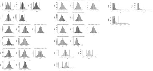
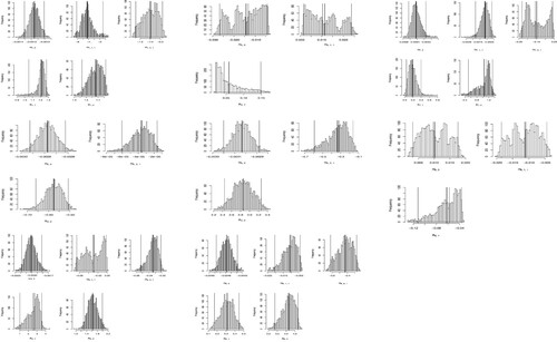
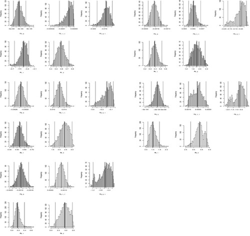
After specifying priors, the Hamiltonian Monte Carlo has been used for obtaining one thousand posterior draws of parameters including $s_1^2$ by using first five-hundred draws as the burn-in. The depiction of the histograms of different parameters is given in Figure 1, whereas the means and the posterior predictive intervals for each ϑ are depicted in Figure 2.

Figure 1. Histograms of posterior parameters.

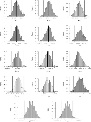
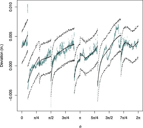
Figure 2. Deviation and model fit for different radius manufactured cylinders assuming logistic errors. (a) Radius $={0.5}^{″}$, (b) radius $={1.5}^{″}$ and (c) radius $={3.0}^{″}$.

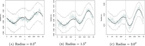
Figure 2 illustrates the model fitted with deviations for three manufactured cylinders, where on the y-axis deviations in inches are plotted against the angle ϑ on the x-axis. The grey dots represent the observed deviations, the solid lines are the means of the posterior predictive distribution, the dashed lines represent 95% posterior predictive intervals while the dashed vertical lines represent the upper and lower halves. For all the assumed radiuses, it can be seen that the observed deviations are within the given limits and close to the posterior predictive means. From Figure 2, it can also be seen that by increasing the radius of the manufactured cylinder shapes, the deviations tend to be positive rather than negative, however, the deviations remain inside the 95% posterior predictive intervals.

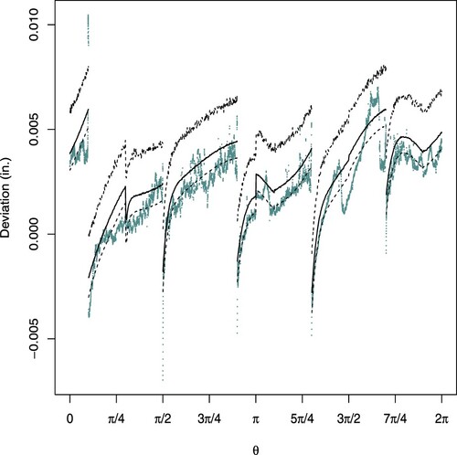
Figure 3 illustrates the fitted deviation model for three manufactured cylinders by utilizing Equation (2(2) ${\mathrm{\nabla }}_1\left(\vartheta \right)={\delta }_1\left(\vartheta |\text{β}\right)+{\mathcal{E}}_1\left(\vartheta \right)$(2) ) with ${\mathcal{E}}_1\left(\vartheta \right)\sim Laplace\left(0,s_1^2\right)$. In Figure 3, for three cylinders, it is found that the observed deviations are within the given limits and are right on the centre of the posterior predictive intervals. Furthermore, we noticed that by increasing the radius of the manufactured cylinder shapes the deviations tend to be positive rather than negative. Contrary to Figure 2, it is observed that the deviation model provides approximately good fit because a very few deviations are near to the limits.

Figure 3. Deviation and model fit for three manufactured cylinders assuming Laplace errors. (a) Radius $={0.5}^{″}$, (b) radius $={1.5}^{″}$ and (c) radius $={3.0}^{″}$.

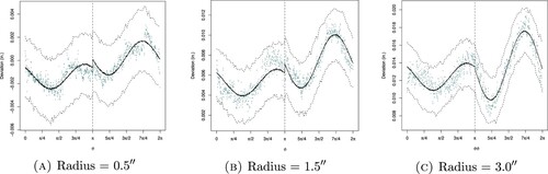
Figure 4 illustrates fitted deviations model for three manufactured cylinders by utilizing Equation (2(2) ${\mathrm{\nabla }}_1\left(\vartheta \right)={\delta }_1\left(\vartheta |\text{β}\right)+{\mathcal{E}}_1\left(\vartheta \right)$(2) ) with ${\mathcal{E}}_1\left(\vartheta \right)\sim Cauchy\left(0,s_1^2\right)$. It is noticed from the figure that the observed deviations are within the given limits and are right on the centre of the posterior predictive intervals and by increasing the radius of the manufactured cylinder shapes, the deviations tend to be positive rather than negative. Further, the deviations are within the 95% posterior predictive intervals. Contrary to Figures 4 and 2, the deviations are very small and have a trend but posterior predictive means and posterior predictive intervals have no specific pattern. The posterior predictive means fluctuate and sometimes fall outside the posterior predictive intervals and predictive means and intervals have no constant mean and constant variance over the angles. Thus, Cauchy distribution for the errors is not suitable as the logistic or Laplace distribution.

Figure 4. Deviation and model fit for three manufactured cylinders assuming Cauchy distributed errors. (a) Radius $={0.5}^{″}$, (b) radius $={0.5}^{″}$, (c) radius $={1.5}^{″}$, (d) radius $={1.5}^{″}$, (e) radius $={3.0}^{″}$ and (f) radius $={3.0}^{″}$.

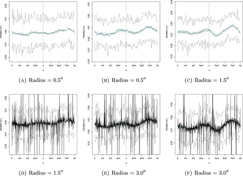
Figure 5 illustrates the deviation model fitted for three manufactured cylinders by utilizing Equation (2(2) ${\mathrm{\nabla }}_1\left(\vartheta \right)={\delta }_1\left(\vartheta |\text{β}\right)+{\mathcal{E}}_1\left(\vartheta \right)$(2) ) with ${\mathcal{E}}_1\left(\vartheta \right)\sim Exp\left(\frac{1}{s_1^2}\right)$. From the figure, for three cylinders, it is found that the observed deviations fall outside the lower limit of the posterior predictive intervals and by increasing the radius of the manufactured cylinder shapes the deviations tend to be positive rather than negative. Furthermore, the posterior predictive means are very close to the lower limit of the posterior predictive interval. There are variations in the upper limit of the posterior predictive intervals but not in the lower limit. The reason behind this is the exponential distribution which is a positively skewed distribution.

Figure 5. Deviation and model fit for three manufactured cylinders assuming exponentially distributed errors. (a) Radius $={0.5}^{″}$, (b) radius $={1.5}^{″}$ and (c) radius $={3.0}^{″}$.

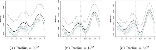
Figure 6 illustrates the fitted deviation model for three manufactured cylinders by utilizing Equation (2(2) ${\mathrm{\nabla }}_1\left(\vartheta \right)={\delta }_1\left(\vartheta |\text{β}\right)+{\mathcal{E}}_1\left(\vartheta \right)$(2) ) with ${\mathcal{E}}_1\left(\vartheta \right)\sim lognormal\left(0,s_1^2\right)$. It is noticed that the observed deviations exactly follow the predictive mean and thus lognormal is also a suitable distribution for the error terms.

Figure 6. Deviation and model fit for three manufactured cylinders.

3.2. Local deviation feature modelling for regular five-sided polygon

To define the local deviation model for regular five-sided polygon, let the nominal radius function be given by ${\mathrm{{\rm Y}}}_2^{nom}\left(\vartheta \right)=\frac{3\cos \left(\frac{\pi }{5}\right)}{\cos \left\{\left(\vartheta -\frac{\pi }{2}\right)mod\frac{2\pi }{5}-\frac{\pi }{5}\right\}}$ where ${\gamma }_2$ = (5,3). Then, the local deviation feature model can be written as ${\delta }_2\left(\vartheta |\alpha \right)=\sum _{k=1}^2\mathbb{I}\left(\vartheta \in {\mathrm{\Theta }}_k\right){\delta }_{2,k}\left(\vartheta |{\alpha }_{e\left(\vartheta \right),k}\right)$ where (6) $\begin{array}{rl}{\delta }_{2,k}\left(\vartheta |{\alpha }_{e\left(\vartheta \right),k}\right)& ={\alpha }_{e\left(\vartheta \right),0}+{\alpha }_{e\left(\vartheta \right),1}\{{\mathrm{{\rm Y}}}_2^{nom}\left(\vartheta \right)\\ & -{{\mathrm{{\rm Y}}}_2^{nom}\left(m\left(\vartheta \right)\right)\}}^{a_{e\left(\vartheta \right),k}}\end{array}$(6) with $m:\left[0,2\pi \right]\to \left[0,2\pi \right]$ defined as $m\left(\vartheta \right)=\underset{t:e\left(t\right)=e\left(\vartheta \right)}{\arg min}{\mathrm{{\rm Y}}}_2^{nom}\left(t\right)$ and $e:\left[0,2\pi \right]\to \left\{1,2,3,4,5\right\}$ is the functional form which returns the block comprising ϑ. For each blocks, five new parameters are introduced which are ${\alpha }_{e\left(\vartheta \right),1,1}$, $a_{e\left(\vartheta \right),1}$ and ${\alpha }_{e\left(\vartheta \right),2,1}$, $a_{e\left(\vartheta \right),2}$ to determine systematic patterns which occur across blocks.

The distinct magnitudes for each pattern across blocks are entertained through the specification of hierarchical models on ${\text{β}}_{e\left(\vartheta \right),0}$, ${\alpha }_{e\left(\vartheta \right),1,1}$. We assume weakly informative priors on $a_{e\left(\vartheta \right),1}$ and $a_{e\left(\vartheta \right),2}$. Furthermore, $\begin{array}{rl}& {\alpha }_{1,0},{\alpha }_{2,0},{\alpha }_{3,0},{\alpha }_{4,0}.{\alpha }_{5,0}\stackrel{iid}{\sim }N\left({\mu }_0,r_0^2\right)\\ & {\alpha }_{1,1,1},{\alpha }_{2,1,1},{\alpha }_{3,1,1},{\alpha }_{4,1,1}.{\alpha }_{5,1,1}\stackrel{iid}{\sim }N\left({\mu }_1,r_1^2\right)\\ & {\alpha }_{1,2,1},{\alpha }_{2,2,1},{\alpha }_{3,2,1},{\alpha }_{4,2,1}.{\alpha }_{5,2,1}\stackrel{iid}{\sim }N\left({\mu }_2,r_2^2\right)\\ & a_{1,0},a_{2,1},\dots ,a_{5,1},a_{1,2},a_{2,2},\dots ,a_{5,2}\stackrel{iid}{\sim }N\left(\frac{1}{2},1^2\right)\end{array}$ The standard reference prior [10] is specified as $p\left(m_0,m_1,m_2,r_0^2,r_1^2,r_2^2\right)\propto \frac{1}{r_0,r_1,r_2}$ To this end, we fit the following model to all the preceding shapes with priors on $\text{β},\alpha ,$ and $s_0^2$, with $\begin{array}{rl}& {\mathrm{\nabla }}_1\left(\vartheta \right)={\delta }_1\left(\vartheta |\text{β}\right)+{\mathcal{E}}_1\left(\vartheta \right)\\ & {\mathrm{\nabla }}_2\left(\vartheta \right)={\delta }_1\left(\vartheta |\text{β}\right)+{\delta }_2\left(\vartheta |\alpha \right)+{\mathcal{E}}_2\left(\vartheta \right)\end{array}$ where errors ${\mathcal{E}}_1\left(\vartheta \right)\sim Logistic\left(0,s_1^2\right)$ and ${\mathcal{E}}_2\left(\vartheta \right)\sim Logistic\left(0,s_2^2\right)$ are mutually independent, and a flat prior is assumed on $\log \left(s_2\right)$. 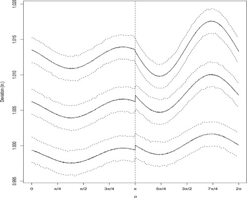To obtain the posterior distribution of α, deviation data for both the new regular pentagon and the cylinders are mixed under this model. To this end, Hamiltonian Monte Carlo is utilized for calculating a thousand posterior draws of parameters α obtained after discarding five hundred observations as the burn-in period (Figure 7).

Figure 7. Histograms of posterior draws for five-sided polygon.

The resulting deviations with posterior predictive means for each block are shown in Figure 8(a) assuming logistic error. Similarly, the summary of the specification of hierarchical model for ${\delta }_2$ of a regular pentagon is depicted in Figure 8(b).

Figure 8. Deviation profile and model fit of a new regular five-sided polygon (pentagon) of size $3^{″}$ assuming logistic error. (a) Deviation profile assuming l Logistic error and (b) deviation and model fit assuming logistic error.

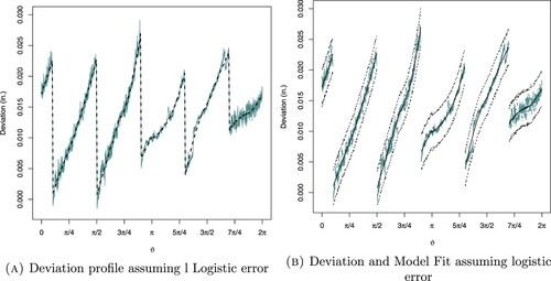
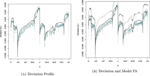
Figure 8(b) illustrates the fitted model with local deviations for regular pentagon assuming logistic errors and it is noticed that the observed deviations are within the 95% posterior predictive interval.

Figure 9(a) illustrates the fitted local deviations model for regular pentagon by utilizing Equation (3(3) ${\mathrm{\nabla }}_2\left(\vartheta \right)={\delta }_1\left(\vartheta |\text{β}\right)+{\delta }_2\left(\vartheta |\alpha \right)+{\mathcal{E}}_2\left(\vartheta \right)$(3) ) with ${\mathcal{E}}_2\left(\vartheta \right)\sim Laplace\left(0,s_2^2\right)$. In Figure 9(b), for each block in a regular pentagon of radius of $3^{″}$, it is noticed that the observed deviations are within the 95% posterior predictive interval. In contrast to Figure 8(b), we noticed that the deviation model provides approximately good fit because a very few deviations are close to the limits.

Figure 9. Deviation profile and model fit of a new regular five-sided polygon (pentagon) of size $3^{″}$ assuming Laplace error. (a) Deviation profile assuming Laplace error and (b) deviation and model fit assuming Laplace error.

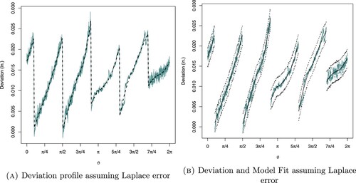
Figure 10 illustrates the fitted local deviations model for regular pentagon by utilizing Equation (3(3) ${\mathrm{\nabla }}_2\left(\vartheta \right)={\delta }_1\left(\vartheta |\text{β}\right)+{\delta }_2\left(\vartheta |\alpha \right)+{\mathcal{E}}_2\left(\vartheta \right)$(3) ) with ${\mathcal{E}}_2\left(\vartheta \right)\sim Cauchy\left(0,s_2^2\right)$. From the figure, for each block in a regular pentagon of radius of 3 inches, it is found that the observed deviations are within the 95% posterior predictive interval. In contrast to Figures 2 and 8, it can be seen that the deviations are very small and show trend but posterior predictive means and posterior predictive intervals have no specific pattern. The posterior predictive means fluctuate and go outside the posterior predictive intervals and there are huge variations in posterior predictive means. Thus, the posterior predictive means and posterior predictive intervals have no constant mean and variance over the angle. Therefore, the posterior predictive means and posterior predictive intervals cannot be correctly estimated.

Figure 10. Deviation and model fit of the new $3^{″}$ regular Pentagon assuming Cauchy distribution for error. (a) Deviation profile assuming Cauchy error, (b) deviation and model fit assuming Cauchy error and (c) deviation and model fit assuming Cauchy error.

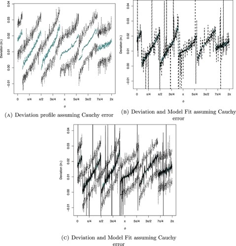
Figure 11(a) depicts the fitted local deviations model for a regular pentagon by utilizing Equation (3(3) ${\mathrm{\nabla }}_2\left(\vartheta \right)={\delta }_1\left(\vartheta |\text{β}\right)+{\delta }_2\left(\vartheta |\alpha \right)+{\mathcal{E}}_2\left(\vartheta \right)$(3) ) with ${\mathcal{E}}_2\left(\vartheta \right)\sim Exp\left(\frac{1}{s_2^2}\right)$. For a regular pentagon, it is noticed that the observed deviations fall outside the lower limit of the posterior predictive intervals. The posterior predictive means are very close to the lower limit of the posterior predictive interval and there are variations in the upper limit of the posterior predictive intervals. The reason behind this pattern is the exponential distribution which is a positively skewed distribution. Figure 12 illustrates the deviation fitted model for regular pentagon by utilizing Equation (3(3) ${\mathrm{\nabla }}_2\left(\vartheta \right)={\delta }_1\left(\vartheta |\text{β}\right)+{\delta }_2\left(\vartheta |\alpha \right)+{\mathcal{E}}_2\left(\vartheta \right)$(3) ) with ${\mathcal{E}}_1\left(\vartheta \right)\sim lognormal\left(0,s_2^2\right)$. This figure shows inappropriate fitting of the model and the deviation model does not perform well assuming lognormal distribution for errors.

Figure 11. Deviation profile and model fit of the new $3^{″}$ regular Pentagon using exponential distribution. (a) Deviation profile of a new $3^{″}$ Pentagon using exponential distribution and (b) deviation and model fit of the new $3^{″}$ regular Pentagon using exponential distribution.

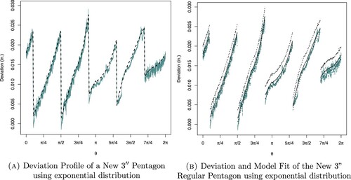
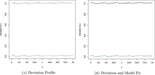
Figure 12. Deviation profile and model fit of the new $3^{″}$ regular Pentagon assuming Lognormal errors. (a) Deviation profile and (b) deviation and model fit.

3.3. An irregular octagon and local deviation feature model

Sabbaghi et al. [10] investigated the model of the local deviation feature for irregular octagon of nominal radius $1^{″}$. However, we noticed wider deviations by considering normally distributed error term. To improve the accuracy of the deviation model, we investigate the impact of different skewed distributions. The utilization of the Bayesian method on a single new regular pentagon and cylinders clearly increases up the need of building the local deviation feature model for more common polygon shapes. To this end, we utilize the existed data library of $D_{current}=\left(D_1,D_2\right)$, ${\delta }_{current}=\left({\delta }_1,{\delta }_2\right)$ and ${\alpha }_{current}$ to identify a model of deviation for any irregular or regular polygon (convex), without any other posterior predictive checks. The reason behind this is polygons (convex) are comprised exclusively straight edges. Therefore, the deviation can be modelled through the simple augmentation of the existed library of functional forms for straight sides. Assume a curved E-sided polygon with the nominal radius ${\mathrm{{\rm Y}}}_3^{nom}\left(\vartheta \right):\left[0,2\pi \right]\to \mathbb{R}$. From the existed data library, it is noticed that the sides constitute blocks and we fix $e:\left[0,2\pi \right]\to \left\{1,\dots ,E\right\}$ as the functional form that gives the block level for each ϑ. Likewise, utilizing the existed information to characterize $m:\left[0,2\pi \right]\to \left[0,2\pi \right]$ as $m\left(\vartheta \right)=\underset{t:e\left(t\right)=e\left(\vartheta \right)}{\arg min}{\mathrm{{\rm Y}}}_3^{nom}\left(t\right)$ and the clusters ${\mathrm{\Theta }}_1=\left\{\vartheta \in \left[0,2\pi \right]:\vartheta >m\left(\vartheta \right)\right\}$, ${\mathrm{\Theta }}_2=\left\{\vartheta \in \left[0,2\pi \right]:\vartheta \le m\left(\vartheta \right)\right\}$. Finally, we extend the previously learned local deviation feature model to ${\mathrm{{\rm Y}}}_3^{nom}(\cdot )$ as (7) ${\delta }_3\left(\vartheta |\alpha \right)=\sum _{k=1}^2\mathbb{I}\left(\vartheta \in {\mathrm{\Theta }}_k\right){\delta }_{3,k}\left(\vartheta |{\alpha }_{e\left(\vartheta \right),k}\right)$(7) with (8) $\begin{array}{rl}{\delta }_{3,k}\left(\vartheta |{\alpha }_{e\left(\vartheta \right),k}\right)& ={\alpha }_{e\left(\vartheta \right),0}+{\alpha }_{e\left(\vartheta \right),1}\{{\mathrm{{\rm Y}}}_3^{nom}\left(\vartheta \right)\\ & -{{\mathrm{{\rm Y}}}_3^{nom}\left(m\left(\vartheta \right)\right)\}}^{a_{e\left(\vartheta \right),k}}\end{array}$(8) We run the local deviation model utilizing data from the previously developed cylinders and a freshly constructed regular pentagon. The irregular octagon does not necessarily have a circumcircle, therefore, one can utilize the minimum bounding circle for the global deviation feature. The model of local deviation feature for irregular octagon can be written as (9) ${\mathrm{\nabla }}_3\left(\vartheta \right)={\delta }_1\left(\vartheta |\text{β}\right)+{\delta }_3\left(\vartheta |\alpha \right)+{\mathcal{E}}_3\left(\vartheta \right)$(9) where ${\delta }_1\left(\vartheta |\text{β}\right)$ is already defined, ${\delta }_3\left(\vartheta |\alpha \right)$, and ${\mathcal{E}}_3\left(\vartheta \right)\sim Logistic\left(0,s_3^2\right)$. A Bayesian hierarchical model is constructed on α, and weakly informative priors on $a_{e\left(\vartheta \right),1},a_{e\left(\vartheta \right),2},$ β, $s_3^2$ are assumed for the analysis. We used the Hamiltonian Monte Carlo for calculating a thousand posterior draws obtained after the burn-in of five hundred draws (Figure 13).

Figure 13. Histograms of posterior parameters for the irregular octagon.

The fitted model for the irregular octagon is plotted in Figure 14(a,b) for the irregular octagon deviation profile, particularly by considering three cylinders and one regular pentagon.

Figure 14. Deviation and model fit for new irregular octagon assuming logistic errors. (a) Deviation profile and (b) deviation and model fit.

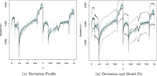
Figure 15 illustrates the local deviation fitted model for irregular octagon by using Equation (4(4) $T_2\left(\vartheta \right)={\mathrm{\nabla }}_2\left(\vartheta \right)-{\delta }_1\left(\vartheta |\widetilde{\text{β}}\right)$(4) ) with ${\mathcal{E}}_3\left(\vartheta \right)\sim Cauchy\left(0,s_3^2\right)$. It is noticed that Cauchy distribution is not appropriate for the errors.

Figure 15. Deviation and model fit for new irregular octagon. (a) Deviation profile and (b) deviation model fit.

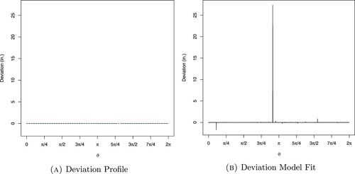
Figure 16(b) illustrates the fitted local deviations model for the irregular octagon by using Equation (4(4) $T_2\left(\vartheta \right)={\mathrm{\nabla }}_2\left(\vartheta \right)-{\delta }_1\left(\vartheta |\widetilde{\text{β}}\right)$(4) ) with ${\mathcal{E}}_3\left(\vartheta \right)\sim Exp\left(\frac{1}{s_3^2}\right)$. From the figure, it can be seen that the observed deviations fall outside the lower limit of the posterior predictive intervals, whereas the posterior predictive means are very close to the lower limit of the posterior predictive interval but not to the upper limit. The fluctuation in the upper limits of the posterior predictive intervals indicates variations in the pattern while the lower limit of the posterior predictive intervals shows smoothness in pattern.

Figure 16. Deviation profile and model fit assuming exponential distribution for errors. (a) Deviation profile and (b) deviation and model fit.

3.4. Free-form shapes with straight edges and local deviation feature model

Sabbaghi et al. [10] also studied the model of the local deviation feature for the free-form shape by assuming normally distributed errors. However, large deviations were noticed in the predictive intervals because of normal distribution of errors. Therefore, we use different error distributions to minimize the predictive intervals. The existed library for models of local deviation feature can be used to study the polygonal shapes. That is, if a new shape's components associate to the existed library, then deviations can be modelled by applying the functions from ${\delta }_{current}$. To this end, the posterior draws for model parameters are depicted in Figure 17.

Figure 17. Histograms of posterior draws for free-form shapes.

The observed deviation is defined as (10) $\begin{array}{rl}& {\mathrm{\nabla }}_4(\vartheta {)=\mathrm{{\rm Y}}}_4^{obs}(\vartheta {)-\mathrm{{\rm Y}}}_4^{nom}(\vartheta )\end{array}$(10) (11) $\begin{array}{rl}& {\mathrm{\nabla }}_3\left(\vartheta \right)={\delta }_1\left(\vartheta |\text{β}\right)+{\delta }_4\left(\vartheta |\alpha \right)+{\mathcal{E}}_4\left(\vartheta \right)\end{array}$(11) where ${\mathcal{E}}_4\left(\vartheta \right)\sim Logistic\left(0,s_4^2\right)$

Figure 18 illustrates the model fitted with local deviations for free form shape. From this figure, it is noticed that the observed deviations are within the 95% posterior predictive interval. However, it is also observed that the deviation model is poorly fitted to the points situated on curved segments because free form shapes would never allow us to understand the deviation characteristic for the curved segments.

Figure 18. Deviation and model fit of the freestyle shape using logistic errors.

Next, Figure 19 illustrates the local deviations model fitted for free form shapes by utilizing Equation (6(6) $\begin{array}{rl}{\delta }_{2,k}\left(\vartheta |{\alpha }_{e\left(\vartheta \right),k}\right)& ={\alpha }_{e\left(\vartheta \right),0}+{\alpha }_{e\left(\vartheta \right),1}\{{\mathrm{{\rm Y}}}_2^{nom}\left(\vartheta \right)\\ & -{{\mathrm{{\rm Y}}}_2^{nom}\left(m\left(\vartheta \right)\right)\}}^{a_{e\left(\vartheta \right),k}}\end{array}$(6) ) with ${\mathcal{E}}_4\left(\vartheta \right)\sim Cauchy\left(0,s_4^2\right)$. From the figure, it is noticed that the observed deviations are within the 95% posterior predictive interval and contrary to Figure 18, the deviations are very small and are showing trend but the posterior predictive means and posterior predictive intervals have no pattern. The posterior predictive means fluctuate very much and fall outside the posterior predictive intervals.

Figure 19. Deviation and model fit for the new freestyle shape using Cauchy Errors. (a) Deviation with posterior predictive Intervals, (b) deviations and posterior predictive means and (c) deviations with posterior predictive means and intervals.

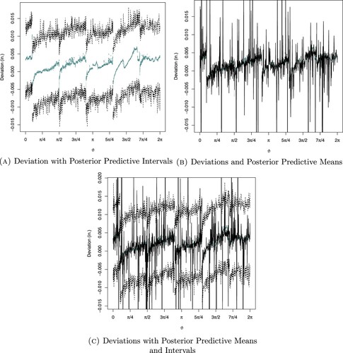
Figure 20 illustrates the local deviations model for free form shapes by using Equation (6(6) $\begin{array}{rl}{\delta }_{2,k}\left(\vartheta |{\alpha }_{e\left(\vartheta \right),k}\right)& ={\alpha }_{e\left(\vartheta \right),0}+{\alpha }_{e\left(\vartheta \right),1}\{{\mathrm{{\rm Y}}}_2^{nom}\left(\vartheta \right)\\ & -{{\mathrm{{\rm Y}}}_2^{nom}\left(m\left(\vartheta \right)\right)\}}^{a_{e\left(\vartheta \right),k}}\end{array}$(6) ) with ${\mathcal{E}}_4\left(\vartheta \right)\sim Exp\left(\frac{1}{s_4^2}\right)$. It is observed from the figure that the observed deviations fall outside the lower limit of the posterior predictive intervals whereas the posterior predictive means are very close to the lower limit of the posterior predictive intervals but not close to the upper limit. The fluctuation in the upper limits of the posterior predictive intervals indicates variations in the pattern while the lower limits of the posterior predictive intervals show a smoothed pattern.

Figure 20. Deviation and model fit for free-form shape assuming exponential errors.

4. Conclusion and recommendations

The results of the fitted model with global deviations assuming logistic, Laplace, Cauchy and exponential distributions of error term for three manufactured cylinders are discussed in this study using the Bayesian deviation model. It is observed that for smaller radius, negative deviations are found whereas for higher radius of the cylinder, the values fall away from the means of posterior predictive distribution. Furthermore, we observed that the deviation model works efficiently for the four straight edges, whereas the model of deviation have a poor fit for points on the bending section. Assuming different distributions for errors, freestyle shapes do not allow to understand the deviation features for the bending section.

The Laplace distribution is also used for errors, which shows that the Bayesian deviation model is approximately a good fit. Likewise, Cauchy distribution is also employed, which shows the lack of fitness of the Bayesian deviation model. The posterior predictive means fluctuate very much and go outside the posterior predictive intervals, and there are huge variations in the posterior predictive means. Furthermore, exponential distribution also shows the lack of fitness because deviations are lying outside in the lower limit of the interval. Also, the means of the posterior predictive distribution are very close to the lower limit. Finally, for the lognormal distribution, it is noticed that the Bayesian deviation model is fitted very poorly.

It is recommended that the fitted model assuming the logistic distribution of the error term with global deviations for three manufactured cylinders and local deviations for regular pentagon, irregular octagon, and free form shapes shows a better fit and should be used rather than assuming other distributions. In future, the performance of other deviation models [33] and discrepancy measures may be studied.

Disclosure statement

No potential conflict of interest was reported by the author(s).

References

- Oliveira JP, LaLonde AD, Ma J. Processing parameters in laser powder bed fusion metal additive manufacturing. Materials Design. 2020;193:108762.
- Oliveira JP, Santos TG, Miranda RM. Revisiting fundamental welding concepts to improve additive manufacturing: from theory to practice. Progress Materials Sci. 2020;107:100590.
- Shen J, Zeng Z, Nematollahi M, et al. In-situ synchrotron X-ray diffraction analysis of the elastic behaviour of martensite and H-phase in a NiTiHf high temperature shape memory alloy fabricated by laser powder bed fusion. Add Manuf Lett. 2021;1:100003.
- Lopes JG, Machado CM, Duarte VR, et al. Effect of milling parameters on HSLA steel parts produced by wire and arc additive manufacturing (WAAM). J Manuf Process. 2020;59:739–749.
- Campbell T, Williams C, Ivanova O, et al. Could 3D printing change the world. In: Technologies, potential, and implications of additive manufacturing. Washington, DC: Atlantic Council; 2011. p. 3.
- Tong K, Amine Lehtihet E, Joshi S. Parametric error modeling and software error compensation for rapid prototyping. Rapid Prototyping J. 2003;9(5):301–313.
- Tong K, Joshi S, Amine Lehtihet E. Error compensation for fused deposition modeling (FDM) machine by correcting slice files. Rapid Prototyping J. 2008;14(1):4–14.
- Huang Q, Zhang J, Sabbaghi A, et al. Optimal offline compensation of shape shrinkage for three-dimensional printing processes. IIE Trans. 2015;47(5):431–441.
- Huang Q, Nouri H, Xu K, et al. Statistical predictive modeling and compensation of geometric deviations of three-dimensional printed products. J Manuf Sci Eng. 2014;136(6):061008.
- Sabbaghi A, Huang Q, Dasgupta T. Bayesian model building from small samples of disparate data for capturing in-plane deviation in additive manufacturing. Technometrics. 2018;60(4):532–544.
- Wang W, Cheah C, Fuh J, et al. Influence of process parameters on stereolithography part shrinkage. Materials Design. 1996;17(4):205–213.
- Sharon E, Mumford D. 2d-shape analysis using conformal mapping. Int J Comput Vision. 2006;70(1):55–75.
- Jin Y, Qin SJ, Huang Q. Offline predictive control of out-of-plane shape deformation for additive manufacturing. J Manuf Sci Eng. 2016;138(12):121005.
- Huang Q. An analytical foundation for optimal compensation of three-dimensional shape deformation in additive manufacturing. J Manuf Sci Eng. 2016;138(6):061010.
- Zhu Z, Anwer N, Mathieu L. Deviation modeling and shape transformation in design for additive manufacturing. Procedia CIRP. 2017;60:211–216.
- Castillo E, Colosimo BM. Statistical shape analysis of experiments for manufacturing processes. Technometrics. 2011;53(1):1–15.
- Zhou C, Chen Y. Additive manufacturing based on optimized mask video projection for improved accuracy and resolution. J Manuf Processes. 2012;14(2):107–118.
- Gebhardt A, Fateri M. 3D printing and its applications. RTejournal-Forum Rapid technol. 2013;2014:1–9.
- Sabbaghi A, Dasgupta T, Huang Q, et al. Inference for deformation and interference in 3D printing. Ann Appl Statist. 2014;8(3):1395–1415.
- Sköld G, Vidarsson H. Analysing the potentials of 3D-printing in the construction industry: considering implementation characteristics and supplier relationship interfaces. Gothenburg: Chalmers University of Technology; 2015.
- Gelman A, Hill J. Data analysis using regression and hierarchical/multilevel models. New York (NY): Cambridge; 2007.
- Park DK, Gelman A, Bafumi J. Bayesian multilevel estimation with poststratification: state-level estimates from national polls. Political Anal. 2004;12(4):375–385.
- Berger JO. Prior information and subjective probability. In: Berger JO, editor. Statistical decision theory and bayesian analysis. New York: Springer; 1985. p. 74–117.
- Oman SD. Specifying a prior distribution in structured regression problems. J Amer Statist Assoc. 1985;80(389):190–195.
- Gelman A, Jakulin A, Pittau MG, et al. A weakly informative default prior distribution for logistic and other regression models. Ann Appl Statist. 2008;2(4):1360–1383.
- Ghaderinezhad F, Ley C. On the impact of the choice of the prior in bayesian statistics. In: Tang N, editor. Bayesian inference on complicated data. Rijeka: IntechOpen; 2020. Available from: https://doi.org/10.5772/intechopen.88994.
- Chen MH, Ibrahim JG, Yiannoutsos C. Prior elicitation, variable selection and bayesian computation for logistic regression models. J R Statist Soc Ser B (Statistical Methodol). 1999;61(1):223–242.
- Rafique M, Ali S, Shah I, et al. A comparison of different bayesian models for leukemia data. Amer J Math Manag Sci. 2021;41(3):244–258.
- Huang Q, Nouri H, Xu K, et al. Predictive modeling of geometric deviations of 3d printed products-a unified modeling approach for cylindrical and polygon shapes. 2014 IEEE International Conference on Automation Science and Engineering (CASE). Silver Spring (MD): IEEE; 2014. p. 25–30.
- Rubin DB. Bayesianly justifiable and relevant frequency calculations for the applied statistician. Ann Statist. 1984;12(4):1151–1172.
- Meng XL. Posterior predictive p-values. Ann Statist. 1994;22(3):1142–1160.
- Reichl J. Estimating marginal likelihoods from the posterior draws through a geometric identity. Monte Carlo Methods Appl. 2020;26(3):205–221.
- Zhu Z, Anwer N, Mathieu L. Geometric deviation modeling with statistical shape analysis in design for additive manufacturing. Procedia CIRP. 2019;84:496–501.