A novel spectral technique for 2D fractional telegraph equation models with spatial variable coefficients

Abstract

In this paper, a class of the two-dimensional (2D) mathematical models of the time fractional telegraph equation with spatial variable coefficients is considered. These models include the 2D time fractional telegraph equation (2D-TFTE), the 2D time fractional diffusion wave equation with damping (2D-TFDWED) and the 2D time fractional wave equation (2D-TFWE). The fractional derivatives are described in the Caputo sense. A novel spectral technique is used to solve the aforementioned models. The technique is based on the operational matrices of the shifted Gegenbauer polynomials in conjunction with the spectral tau method. The product of operational matrices of the space vectors is constructed in a simple way to remove the obstacle that facing the use of the tau method in solving the variable coefficients fractional/integer order PDEs. Miscellaneous numerical experiments are offered to verify the accuracy and rapid rate of convergence of the presented numerical technique.

Keywords:

• 2D-TFTE models
• operational matrices
• tau method
• Gegenbauer polynomials

1. Introduction

Fractional calculus is one of the most interdisciplinary fields of applied mathematics which has attracted the attentions of many researchers. The memory and the nonlocal property of the fractional calculus make it more accurate than the classical (integer-order) calculus for mathematical modelling of many various phenomena in bioscience [1], hydrology [2], quantum mechanics [3], engineering [4], physics [5,6], electro-chemistry [7], finance [8] and many other fields. The fractional mathematical models described by fractional ordinary or partial differential equations demonstrate the properties of real-world phenomena in a comprehensive and accurate manner [9–14]. So far there have been several fundamental works on the fractional derivative and fractional differential equations [15–19].

In this paper, we consider the 2D-TFPDE model with space variable coefficients in the following form:

(1) $\begin{array}{rl}& {}_0^c{\mathcal{D}}_t^v\mathcal{U}+B_1(x,y){}_0^c{\mathcal{D}}_t^{\eta }\mathcal{U}+B_2(x,y)\mathcal{U}\\ & =B_3(x,y)\frac{{\mathrm{\partial }}^2\mathcal{U}}{\mathrm{\partial }{x}^2}+B_4(x,y)\frac{{\mathrm{\partial }}^2\mathcal{U}}{\mathrm{\partial }{y}^2}+f(x,y,t),\\ & (x,y,t)\in \mathrm{\Omega }\times \mathrm{\Lambda },\end{array}$(1) subject to the initial conditions (ICs) and boundary conditions (BCs):

(2) $\{\begin{array}{ll}u(x,y,0)=f_0(x,y),& {\displaystyle \frac{\mathrm{\partial }u(x,y,0)}{\mathrm{\partial }t}}=f_1(x,y),\\ (x,y)\in \mathrm{\Omega },\\ u(0,y,t)=g_0(y,t),& u(L,y,t)=g_1(y,t),\\ (y,t)\in [0,l]\times \mathrm{\Lambda },\\ u(x,0,t)=h_0(x,t),& u(x,l,t)=h_1(x,t),\\ (x,t)\in [0,L]\times \mathrm{\Lambda },\end{array}$(2) where $\mathcal{U}:=u(x,y,t)$, Ω is the finite rectangular region $[0,L]\times [0,l]$ in ${\mathbb{R}}^2$, $\mathrm{\Lambda }=(0,\tau ]$ represents the time interval, $0<\eta \le 1$ and $1<v\le 2$. ${}_0^c{\mathcal{D}}_t^{v}u(x,y,t)$ and ${}_0^c{\mathcal{D}}_t^{\eta }u(x,y,t)$ denote Caputo's fractional derivatives of $u(x,y,t)$ of orders v and η respectively, It is worthy to mention here that the fractional derivative in Caputo sense of any order θ is defined by (3) $\begin{array}{rl}& {}_0^c{\mathcal{D}}_t^{\theta }u(x,y,t)\\ & =\{\begin{array}{l}{\displaystyle \frac{1}{\mathrm{\Gamma }(n-\theta )}}{\displaystyle {\int }_0^t(t-\zeta {)}^{n-\theta -1}}\\ {\displaystyle \frac{{\mathrm{d}}^n}{\mathrm{d}{\zeta }^n}}u(x,y,\zeta )\mathrm{d}\zeta & n-1<\theta <n,\\ & t>0,\\ {\displaystyle \frac{{\mathrm{\partial }}^{n}u\left(t\right)}{\mathrm{\partial }{t}^n}}& \theta =n.\end{array}\end{array}$(3) The fractional mathematical model (1(1) $\begin{array}{rl}& {}_0^c{\mathcal{D}}_t^v\mathcal{U}+B_1(x,y){}_0^c{\mathcal{D}}_t^{\eta }\mathcal{U}+B_2(x,y)\mathcal{U}\\ & =B_3(x,y)\frac{{\mathrm{\partial }}^2\mathcal{U}}{\mathrm{\partial }{x}^2}+B_4(x,y)\frac{{\mathrm{\partial }}^2\mathcal{U}}{\mathrm{\partial }{y}^2}+f(x,y,t),\\ & (x,y,t)\in \mathrm{\Omega }\times \mathrm{\Lambda },\end{array}$(1) ) represents the 2D-TFTE or the 2D-TFDWED for ($B_2(x,y)=0,\eta =1$) while it describes the 2D-TFWE for ($B_2(x,y)=B_1(x,y)=0$).

The 2D-TFTE is basically inferred from the inconstant relationship between current and voltage waves on the proportioned transmission line. It's commonly used for modelling several phenomena in applied fields, for example, blood flow under magnetic and vibration mode in a porous tube with thermochemical properties [20], propagation and transmission of electrical signals [21]. The heat diffusion and wave propagation equations are special cases of the telegraph equation. Indeed, the telegraph equation is more appropriate than the diffusion equation for modelling propagation of the interaction of high-frequency multiconductor transmission lines [22], enhancing denoising of image structure of elastic manifolds [23], bimolecular reactions in homogeneous media [24] and anomalous diffusion [25]. The classical telegraph equation cannot accurately characterize the abnormal propagation phenomenon through finite long transmissions due to some loss of power and signal in the system [26]. Therefore, it was necessary to formulate a kind of equation which can quantify these losses to ensure maximum output at the end. In practical application, these occur in time and (or) space fractional telegraph equation. The 2D-TFDWED represents the motion of waves with damping effect in a string due to the term $B_1(x,y)\frac{\mathrm{\partial }\mathcal{U}}{\mathrm{\partial }t}$. The fractional diffusion wave equation is more accurate for modelling many mechanical responses and acoustic rather than the classical diffusion wave equation [27]. Strictly speaking, the 2D-TFDWED without the free term $f(x,y,t)$ represents the fractional Cattaneo equation. The 2D-TFWE describes the mechanical waves or light waves and appears in many applications like signal propagation in electromagnetic media [28] and fluid dynamics [29].

Recently, considerable attention has been devoted for providing numerical techniques for solving the 2D-TFPDE while finding the exact analytical solution of such equations is almost impossible due to the two fractional derivatives included in the equation. Mohebbi et al. [30] presented the collocation method with radial basis functions to solve the 1D and 2D-TFTE. Hosseini et al. [31] presented an approximate solution of the 2D-TFTE with Dirichlet boundary conditions based on a local radial point interpolation method. Shivanian [32] utilized benefits from spectral collocation and meshless methods for solving the 2D-FTE. Hashemi et al. [33] imposed a fictitious coordinate in the TFTE then for its approximate solution they employed a combination of the group preserving scheme and the method of line. Ajmal [34] developed an iterative method based on the skewed grid Crank–Nicolson finite difference method FSKG (C-N) for solving the 2D-TFTE. Hosseini et al. [35] employed a meshless method based on local radial point interpolation for solving the 2D-TFDWED, they used radial basis function to develop their method for meshless Galerkin weak form technique. Uddin et al. [36] presented a hybrid transform method based on combining Laplace transform with localized meshless method for solving the 2D-TFDWE. Kumar et al. [37] presented a meshless local collocation method of meshless radial basis function for space discretization where the time derivative is approximated by using the finite difference method for solving the 1D and 2D-TFDWE in regular and irregular domains.

Tau, collocation and Galerkin spectral methods represent one of the most effective tools for finding accurate approximate solutions of classical and fractional differential equation with few degrees of freedom of the basis functions. This is due to their implementation in bounded and unbounded area [38–40]. The speed convergence rate is one of the significant benefits of the spectral method. In general, spectral methods are encouraging candidates for solving fractional differential equations since their global character fits substantially with the non-local definition of fractional operators. The utilized basis functions have a major affaire on the preciseness of the approximate solutions. Using orthogonal polynomials such as Gegenbauer, Jacobi, Legendre and Chebyshev polynomials as a basis function gives preferable approximate results. Operational matrices (OMs) were reformed for solving several kinds of fractional differential equations (FDEs). The scheme of numerical techniques of combining with OMs of some orthogonal polynomials for solving FDEs established greatly accurate solutions for such equation [41–43].

Due to the lack of works that present numerical solutions for the 2D-TFPDEs with space variable coefficients, in this paper, we present a new spectral tau algorithm based on SG polynomials to discretize the second-order 2D-TFPDE with space variable coefficients. In the proposed technique, a new construction of the product of the operational matrices of the spatial variable coefficients is established. This construction is used to remove the obstacle that faces the use of the tau method in solving the variable coefficients fractional/integer order PDEs. The proposed method easily fulfils for approximate solution of the proposed problem. It has the ability to convert the given problem into a system of algebraic equations, which is easy to solve. Also, it converges exponentially in temporal discretization. As far as we know, there are no results of the spectral tau method for solving the 2D-TFPDE with space variable coefficients.

The outline of the present work is arranged as follows. In Section 2, we retrieve some pertinent properties of the SG polynomials with the SGOM of Caputo fractional derivative. In Section 3, the producer solution of the proposed SG spectral tau method for the proposed space variable mathematical model is constructed. In Section 4, miscellaneous test examples on the constant and space variable coefficients 2D-TFTE, 2D-TFDWED and 2D-TFWE are presented. Section 5 ends the paper with a conclusion.

2. Shifted Gegenbauer polynomials and fractional derivative operational matrix

Gegenbauer polynomials $C_k^{\left(\alpha \right)}\left(t\right)$ with degree $k\in {\mathbb{Z}}^{\mathbb{+}}$ and parameter $\alpha >-\frac{1}{2}$ are orthogonal polynomials on the interval $[-1,1]$ which can be defined as Taylor coefficients expansion of the following generating function [44]: $(1-2tx+x^2{)}^{-\alpha }=\sum _{k=0}^{\mathrm{\infty }}{C}_k^{\left(\alpha \right)}(t)x^k.$ SG polynomials $C_{\tau ,k}^{\left(\alpha \right)}\left(t\right)$ defined on the interval $[0,\tau ]$ are obtained by making the change of the variable $t\to \frac{2t}{\tau }-1$ of $C_k^{\left(\alpha \right)}\left(t\right)$. The analytic form of the SG polynomials is given by (4) $C_{\tau ,k}^{\left(\alpha \right)}\left(t\right)=\sum _{r=0}^k{\mathrm{{\rm Y}}}_{r,k}{t}^r,0<t<\tau ,$(4) where ${\mathrm{{\rm Y}}}_{r,k}=(-1{)}^{k-r}\frac{k!\mathrm{\Gamma }(\alpha +\frac{1}{2})\mathrm{\Gamma }(k+r+2\alpha )}{\mathrm{\Gamma }(k+\alpha +\frac{1}{2})\mathrm{\Gamma }(k+2\alpha )(k-r)!r!{\tau }^r}.$ The SG polynomials with the weight function ${\omega }_{\tau }^{\alpha }\left(t\right)=(\tau t-t^2{)}^{\alpha -\frac{1}{2}}$ form a complete orthogonal set which satisfies the following property: (5) $\begin{array}{rl}& 〈C_{\tau ,r}^{\left(\alpha \right)}\left(t\right),C_{\tau ,k}^{\left(\alpha \right)}\left(t\right){〉}_{{\omega }_{\tau }^{\alpha }\left(t\right)}\\ & ={\int }_0^{\tau }{C}_{\tau ,r}^{\left(\alpha \right)}\left(t\right)C_{\tau ,k}^{\left(\alpha \right)}\left(t\right){\omega }_{\tau }^{\alpha }\left(t\right)\mathrm{d}t=h_{\tau ,r}^{\left(\alpha \right)}{\delta }_{r,k},\end{array}$(5) where ${\delta }_{r,k}$ is the Kronecker delta and $h_{\tau ,r}^{\left(\alpha \right)}$ is given by (6) $h_{\tau ,r}^{\left(\alpha \right)}=\frac{{\tau }^{2\alpha }(r!){\left(\mathrm{\Gamma }(\alpha +\frac{1}{2})\right)}^2}{2(r+\alpha )\mathrm{\Gamma }(r+2\alpha )}.$(6) It is worth to point out that shifted Legendre polynomials ${\mathcal{L}}_{\tau ,r}\left(t\right)$, shifted Chebyshev polynomials of the first and second kind ${\mathcal{T}}_{\tau ,r}\left(t\right)$, $U_{\tau ,k}\left(t\right)$ of degree k are special cases of SG polynomials $C_{\tau ,r}^{\left(\alpha \right)}\left(t\right)$. More precisely, we have $\begin{array}{rl}{\mathcal{T}}_{\tau ,r}\left(t\right)& =C_{\tau ,r}^{\left(0\right)}\left(t\right),U_{\tau ,r}\left(t\right)=(r+1)C_{\tau ,r}^{\left(1\right)}\left(t\right),\\ {\mathcal{L}}_{\tau ,r}\left(t\right)& =C_{\tau ,r}^{\left(\frac{1}{2}\right)}\left(t\right),r\ge 0.\end{array}$• The SG polynomials can be used to approximate a function $u\left(t\right)\in {\mathcal{L}}_{{\omega }^{\alpha }}^2(0,\tau )$ as follows: (7) $u\left(t\right)=\sum _{k=0}^M{c}_k{C}_{\tau ,k}^{\left(\alpha \right)}\left(t\right)={\mathbf{C}}^T{\varphi }_{\tau ,M}\left(t\right),$(7) where T denotes the transpose, from (5(5) $\begin{array}{rl}& 〈C_{\tau ,r}^{\left(\alpha \right)}\left(t\right),C_{\tau ,k}^{\left(\alpha \right)}\left(t\right){〉}_{{\omega }_{\tau }^{\alpha }\left(t\right)}\\ & ={\int }_0^{\tau }{C}_{\tau ,r}^{\left(\alpha \right)}\left(t\right)C_{\tau ,k}^{\left(\alpha \right)}\left(t\right){\omega }_{\tau }^{\alpha }\left(t\right)\mathrm{d}t=h_{\tau ,r}^{\left(\alpha \right)}{\delta }_{r,k},\end{array}$(5) ) the coefficients $c_k$ can be calculated by (8) $\begin{array}{rl}{c}_k& =\frac{1}{h_{\tau ,k}^{\left(\alpha \right)}}〈u\left(t\right),\\ C_{\tau ,k}^{\left(\alpha \right)}\left(t\right){〉}_{{\omega }_{\tau }^{\alpha }\left(t\right)}& =\frac{1}{h_{\tau ,k}^{\left(\alpha \right)}}{\int }_0^{\tau }u\left(t\right)C_{\tau ,k}^{\left(\alpha \right)}\left(t\right){\omega }_{\tau }^{\left(\alpha \right)}\left(t\right)\mathrm{d}t,\\ k& =0,1,\dots ,M,\end{array}$(8) and (9) $\begin{array}{rl}{\mathbf{C}}^T& \equiv [c_0,c_1,\dots ,c_M],\\ {\varphi }_{\tau ,M}\left(t\right)& \equiv \left[C_{\tau ,0}^{\left(\alpha \right)}\right(t),C_{\tau ,1}^{\left(\alpha \right)}(t),\dots ,C_{\tau ,M}^{\left(\alpha \right)}(t){]}^T.\end{array}$(9) • The function $u(x,y,t)$ where $(x,y,t)\in \mathrm{\Omega }\times \mathrm{\Lambda }$ can be approximated in the matrix form by using Kronecker product of matrices. First, we render that the Kronecker product of a matrix Y of order $(p\times r)$ and a matrix Z of order $(q\times s)$ is a matrix of order $(pq\times rs)$ which has the following block form: $Y\otimes Z=\left(\begin{array}{cccc}{y}_{11}Z& y_{12}Z& \dots & y_{1r}Z\\ y_{21}Z& y_{22}Z& \dots & y_{2r}Z\\ ⋮& ⋮& \ddots & ⋮\\ y_{p1}Z& y_{p2}Z& \dots & y_{pr}Z\end{array}\right),$ where the symbol ⊗ is the Kronecker tensor product, also, the Kronecker product satisfies the following properties for matrices U, V, W and X: (10) $UV\otimes WX=(U\otimes W)(V\otimes X).$(10) Accordingly, the function $u(x,y,t)\in {\mathcal{L}}_{{\omega }^{\alpha }}^2(\mathrm{\Omega }\times \mathrm{\Lambda })$ can be written with the following structure: (11) $\begin{array}{rl}{u}_{N,P,M}(x,y,t)& =\sum _{i=0}^N\sum _{j=0}^P\sum _{k=0}^M{a}_{i,j,k}{C}_{L,i}^{\left(\alpha \right)}\left(x\right)C_{\ell ,j}^{\left(\alpha \right)}\left(y\right)C_{\tau ,k}^{\left(\alpha \right)}\left(t\right)\\ & ={\varphi }_{\tau ,M}^T\left(t\right)\mathbf{A}\left({\varphi }_{L,N}\right(x)\otimes {\varphi }_{L,P}(y\left)\right),\end{array}$(11) where the coefficients matrix $\mathbf{A}$ is written in the block form as (12) $\begin{array}{rl}\mathbf{A}& =[A_0,A_1,\dots ,A_N],A_j=[A_{i,0},A_{i,1},\dots ,A_{i,P}],\\ A_{i,j}& =[a_{i,j,0},a_{i,j,1},\dots ,a_{i,j,M}{]}^T,\end{array}$(12) and the coefficients $a_{i,j,k}$ are calculated by (13) $\begin{array}{rl}{a}_{i,j,k}& =\frac{1}{h_{\tau ,k}^{\left(\alpha \right)}{h}_{L,i}^{\left(\alpha \right)}{h}_{l,j}^{\left(\alpha \right)}}〈〈〈u(x,y,t),C_{\tau ,k}^{\left(\alpha \right)}\left(t\right)C_{L,i}^{\left(\alpha \right)}\left(x\right)\\ & C_{l,j}^{\left(\alpha \right)}\left(y\right){〉}_{{\omega }_L^{\alpha }\left(x\right)}{〉}_{{\omega }_l^{\alpha }\left(y\right)}{〉}_{{\omega }_{\tau }^{\alpha }\left(t\right)}\\ & =\frac{1}{h_{\tau ,k}^{\left(\alpha \right)}{h}_{L,i}^{\left(\alpha \right)}{h}_{l,j}^{\left(\alpha \right)}}{\int }_0^l{\int }_0^L{\int }_0^{\tau }u(x,y,t)C_{\tau ,k}^{\left(\alpha \right)}\left(t\right)C_{L,i}^{\left(\alpha \right)}\left(x\right)\\ & \times C_{l,j}^{\left(\alpha \right)}\left(y\right){\omega }_{\tau }^{\left(\alpha \right)}\left(t\right){\omega }_L^{\left(\alpha \right)}\left(x\right){\omega }_l^{\left(\alpha \right)}\left(y\right)\mathrm{d}t\mathrm{d}x\mathrm{d}y,\end{array}$(13) $i=0,1,\dots ,M,j=0,1,\dots ,N,k=0,1,\dots ,p.$ Now, the construction of SGOM of the Caputo fractional derivative is given from the following theorem.

Theorem 2.1

see [45]

Let ${\varphi }_{\tau ,M}\left(t\right)$ be given as in (9(9) $\begin{array}{rl}{\mathbf{C}}^T& \equiv [c_0,c_1,\dots ,c_M],\\ {\varphi }_{\tau ,M}\left(t\right)& \equiv \left[C_{\tau ,0}^{\left(\alpha \right)}\right(t),C_{\tau ,1}^{\left(\alpha \right)}(t),\dots ,C_{\tau ,M}^{\left(\alpha \right)}(t){]}^T.\end{array}$(9) ) then it's Caputo derivative of fractional order $(\eta >0)$ can be expressed as (14) ${}_0^c{\mathcal{D}}_t^{\eta }{\varphi }_{\tau ,M}\left(t\right)\simeq {\mathbf{D}}_{\tau }^{\left(\eta \right)}{\varphi }_{\tau ,M}\left(t\right)$(14) where ${\mathbf{D}}_{\tau }^{\left(\eta \right)}$ is an $(M+1)$ square matrix of the form (15) $\begin{array}{rl}{\mathbf{D}}_{\tau }^{\left(\eta \right)}& =(\begin{array}{cc}0& 0\\ ⋮& ⋮\\ 0& 0\\ \mathrm{\Theta }(\lceil \eta \rceil ,0,\alpha ,\eta )& \mathrm{\Theta }(\lceil \eta \rceil ,1,\alpha ,\eta )\\ ⋮& ⋮\\ \mathrm{\Theta }(M,0,\alpha ,\eta )& \mathrm{\Theta }(M,1,\alpha ,\eta )\end{array}\\ & \begin{array}{cc}\dots & 0\\ \ddots & ⋮\\ \dots & 0\\ \dots & \mathrm{\Theta }(\lceil \eta \rceil ,M,\alpha ,\eta )\\ \ddots & ⋮\\ \dots & \mathrm{\Theta }(M,M,\alpha ,\eta )\end{array}),\end{array}$(15) where ${\mathbf{D}}_{\tau }^{\left(\eta \right)}=\{\begin{array}{ll}\mathrm{\Theta }(k,j,\alpha ,\eta )& k\ge \lceil \eta \rceil ,\\ 0& k<\lceil \eta \rceil ,\end{array}$ with (16) $\begin{array}{rl}& \mathrm{\Theta }(k,j,\alpha ,\eta )\\ & =\sum _{r=\lceil \eta \rceil }^k{\mathrm{{\rm Y}}}_{r,k}\frac{r!{\tau }^r}{\mathrm{\Gamma }(r+1-\eta )}\sum _{s=0}^j{\mathrm{{\rm Y}}}_{s,j}\\ & \times \frac{2(j+\alpha )\mathrm{\Gamma }(j+2\alpha )\mathrm{\Gamma }(s+r-\eta +\alpha +\frac{1}{2}){\tau }^{s-\eta }}{j!\mathrm{\Gamma }(\alpha +\frac{1}{2})\mathrm{\Gamma }(s+r-\eta +2\alpha +1)}.\end{array}$(16)

3. SG tau method

In this section, the procedures solution of the presented method for solving the 2D-TFPDE model (1(1) $\begin{array}{rl}& {}_0^c{\mathcal{D}}_t^v\mathcal{U}+B_1(x,y){}_0^c{\mathcal{D}}_t^{\eta }\mathcal{U}+B_2(x,y)\mathcal{U}\\ & =B_3(x,y)\frac{{\mathrm{\partial }}^2\mathcal{U}}{\mathrm{\partial }{x}^2}+B_4(x,y)\frac{{\mathrm{\partial }}^2\mathcal{U}}{\mathrm{\partial }{y}^2}+f(x,y,t),\\ & (x,y,t)\in \mathrm{\Omega }\times \mathrm{\Lambda },\end{array}$(1) )–(2(2) $\{\begin{array}{ll}u(x,y,0)=f_0(x,y),& {\displaystyle \frac{\mathrm{\partial }u(x,y,0)}{\mathrm{\partial }t}}=f_1(x,y),\\ (x,y)\in \mathrm{\Omega },\\ u(0,y,t)=g_0(y,t),& u(L,y,t)=g_1(y,t),\\ (y,t)\in [0,l]\times \mathrm{\Lambda },\\ u(x,0,t)=h_0(x,t),& u(x,l,t)=h_1(x,t),\\ (x,t)\in [0,L]\times \mathrm{\Lambda },\end{array}$(2) ) is discussed in detail.

3.1. Functions approximation

First, the functions $B_i(x,y)$ for i = 1, 2, 3, 4 can be approximated by the SG polynomials as follows: (17) $B_{i,N,P}(x,y)={\mathcal{P}}_i^T\left({\varphi }_{L,N}\right(x)\otimes {\varphi }_{l,P}(y\left)\right),$(17) where ${\mathcal{P}}_i$ are column vectors of the following form: (18) $\begin{array}{rl}{\mathcal{P}}_i& =[p_{0,0}^i,p_{0,1}^i,\dots ,p_{0,P}^i,p_{1,0}^i,p_{1,1}^i,\dots ,p_{1,P}^i,\dots ,\\ & p_{N,0}^i,p_{N,1}^i,\dots ,p_{N,P}^i{]}^T,i=1,2,3,4,\end{array}$(18) and its elements can be calculated from (19) $\begin{array}{rl}{p}_{j,k}^i& =\frac{1}{h_{L,j}^{\left(\alpha \right)}{h}_{l,k}^{\left(\alpha \right)}}〈〈B_i(x,y),C_{L,j}^{\left(\alpha \right)}\left(x\right)C_{l,k}^{\left(\alpha \right)}\left(y\right)〉{〉}_{{\omega }_L^{\alpha }\left(x\right){\omega }_l^{\alpha }\left(y\right)}\\ & =\frac{1}{h_{L,j}^{\left(\alpha \right)}{h}_{l,k}^{\left(\alpha \right)}}{\int }_0^l{\int }_0^L{B}_i(x,y)C_{L,j}^{\left(\alpha \right)}\left(x\right)C_{l,k}^{\left(\alpha \right)}\left(y\right){\omega }_L^{\left(\alpha \right)}\\ & \times \left(x\right){\omega }_l^{\left(\alpha \right)}\left(y\right)\mathrm{d}x\mathrm{d}y,\end{array}$(19) $\begin{array}{rl}i& =1,2,3,4,j=0,1,\dots ,N,k=0,1,\dots ,p.\end{array}$ The functions $f(x,y,t),f_0(x,y),f_1(x,y),g_0(y,t),g_1(y,t),h_0(x,t)$ and $h_1(x,t)$ are approximated by the SG polynomials as follows: (20) $\begin{array}{c}\{\begin{array}{l}{f}_{N,P,M}(x,y,t)\simeq {\varphi }_{\tau ,M}^T\left(t\right)\mathbf{F}\left({\varphi }_{L,N}\right(x)\otimes {\varphi }_{l,P}(y\left)\right),\\ f_{0,N,P,M}(x,y)\simeq {\varphi }_{\tau ,M}^T\left(0\right){\mathbf{F}}_0\left({\varphi }_{L,N}\right(x)\otimes {\varphi }_{l,P}(y\left)\right),\\ f_{1,N,P,M}(x,y)\simeq {\varphi }_{\tau ,M}^T\left(0\right){\mathbf{F}}_1\left({\varphi }_{L,N}\right(x)\otimes {\varphi }_{l,P}(y\left)\right),\\ g_{0,N,P,M}(y,t)\simeq {\varphi }_{\tau ,M}^T\left(t\right){\mathbf{G}}_0\left({\varphi }_{L,N}\right(0)\otimes {\varphi }_{l,P}(y\left)\right),\\ g_{1,N,P,M}(y,t)\simeq {\varphi }_{\tau ,M}^T\left(t\right){\mathbf{G}}_1\left({\varphi }_{L,N}\right(L)\otimes {\varphi }_{l,P}(y\left)\right),\\ h_{0,N,P,M}(x,t)\simeq {\varphi }_{\tau ,M}^T\left(t\right){\mathbf{H}}_0\left({\varphi }_{L,N}\right(x)\otimes {\varphi }_{l,P}(0\left)\right),\\ h_{1,N,P,M}(x,t)\simeq {\varphi }_{\tau ,M}^T\left(t\right){\mathbf{H}}_1\left({\varphi }_{L,N}\right(x)\otimes {\varphi }_{l,P}(l\left)\right),\end{array}\end{array}$(20) where $\mathbf{F},{\mathbf{F}}_0,{\mathbf{F}}_1,{\mathbf{G}}_0,{\mathbf{G}}_1,{\mathbf{H}}_0$ and ${\mathbf{H}}_1$ are known block form matrices written likewise Equation (12(12) $\begin{array}{rl}\mathbf{A}& =[A_0,A_1,\dots ,A_N],A_j=[A_{i,0},A_{i,1},\dots ,A_{i,P}],\\ A_{i,j}& =[a_{i,j,0},a_{i,j,1},\dots ,a_{i,j,M}{]}^T,\end{array}$(12) ) and their elements can be calculated likewise Equation (13(13) $\begin{array}{rl}{a}_{i,j,k}& =\frac{1}{h_{\tau ,k}^{\left(\alpha \right)}{h}_{L,i}^{\left(\alpha \right)}{h}_{l,j}^{\left(\alpha \right)}}〈〈〈u(x,y,t),C_{\tau ,k}^{\left(\alpha \right)}\left(t\right)C_{L,i}^{\left(\alpha \right)}\left(x\right)\\ & C_{l,j}^{\left(\alpha \right)}\left(y\right){〉}_{{\omega }_L^{\alpha }\left(x\right)}{〉}_{{\omega }_l^{\alpha }\left(y\right)}{〉}_{{\omega }_{\tau }^{\alpha }\left(t\right)}\\ & =\frac{1}{h_{\tau ,k}^{\left(\alpha \right)}{h}_{L,i}^{\left(\alpha \right)}{h}_{l,j}^{\left(\alpha \right)}}{\int }_0^l{\int }_0^L{\int }_0^{\tau }u(x,y,t)C_{\tau ,k}^{\left(\alpha \right)}\left(t\right)C_{L,i}^{\left(\alpha \right)}\left(x\right)\\ & \times C_{l,j}^{\left(\alpha \right)}\left(y\right){\omega }_{\tau }^{\left(\alpha \right)}\left(t\right){\omega }_L^{\left(\alpha \right)}\left(x\right){\omega }_l^{\left(\alpha \right)}\left(y\right)\mathrm{d}t\mathrm{d}x\mathrm{d}y,\end{array}$(13) ).

3.2. Multiplication of two Kronecker products of space vectors

In this section, we will compute the matrix which approximates the product of two Kronecker products of space vectors.

Consider the smooth and continuous function $B(x,y)$. Therefore, $B(x,y)$ can be approximated by SG polynomials as $B_{N,P}(x,y)={\mathcal{P}}^T\left({\varphi }_{L,N}\right(x)\otimes {\varphi }_{l,P}(y\left)\right)$, now we are looking for an $(N+1)(P+1)$ square matrix $\mathbf{W}$ which satisfies the approximation (21) $\begin{array}{rl}& ({\varphi }_{L,N}\left(x\right)\otimes {\varphi }_{l,P}\left(y\right))({\varphi }_{L,N}\left(x\right)\otimes {\varphi }_{l,P}\left(y\right){)}^T\mathcal{P}\\ & ={\mathbf{W}}^T({\varphi }_{L,N}\left(x\right)\otimes {\varphi }_{l,P}\left(y\right)).\end{array}$(21) The left-hand side of (21(21) $\begin{array}{rl}& ({\varphi }_{L,N}\left(x\right)\otimes {\varphi }_{l,P}\left(y\right))({\varphi }_{L,N}\left(x\right)\otimes {\varphi }_{l,P}\left(y\right){)}^T\mathcal{P}\\ & ={\mathbf{W}}^T({\varphi }_{L,N}\left(x\right)\otimes {\varphi }_{l,P}\left(y\right)).\end{array}$(21) ) can be written as (22) $\begin{array}{rl}& ({\varphi }_{L,N}\left(x\right)\otimes {\varphi }_{l,P}\left(y\right))({\varphi }_{L,N}\left(x\right)\otimes {\varphi }_{l,P}\left(y\right){)}^T\mathcal{P}\\ & =\sum _{i=0}^N\sum _{j=0}^P{p}_{i,j}{C}_{L,i}^{\left(\alpha \right)}\left(x\right)C_{l,j}^{\left(\alpha \right)}\left(y\right)C_{L,r}^{\left(\alpha \right)}\left(x\right)C_{l,s}^{\left(\alpha \right)}\left(y\right).\end{array}$(22) By approximating $C_{L,i}^{\left(\alpha \right)}\left(x\right)C_{l,j}^{\left(\alpha \right)}\left(y\right)C_{L,r}^{\left(\alpha \right)}\left(x\right)C_{l,s}^{\left(\alpha \right)}\left(y\right)$ for $r=0,1,\dots ,N$ and $s=0,1,\dots ,P$ as (23) $\begin{array}{rl}& C_{L,i}^{\left(\alpha \right)}\left(x\right)C_{l,j}^{\left(\alpha \right)}\left(y\right)C_{L,r}^{\left(\alpha \right)}\left(x\right)C_{l,s}^{\left(\alpha \right)}\left(y\right)\\ & =\sum _{p=0}^N\sum _{q=0}^P{\chi }_{p,q}^{i,j,r,s}{C}_{L,p}^{\left(\alpha \right)}\left(x\right)C_{l,q}^{\left(\alpha \right)}\left(y\right)\\ & ={\mathcal{W}}_{i,j,r,s}({\varphi }_{L,N}\left(x\right)\otimes {\varphi }_{l,P}\left(y\right)),\end{array}$(23) where $\begin{array}{rl}{\mathcal{W}}_{i,j,r,s}& =[{\chi }_{0,0}^{i,j,r,s},{\chi }_{0,1}^{i,j,r,s},\dots ,{\chi }_{0,P}^{i,j,r,s},{\chi }_{1,0}^{i,j,r,s},{\chi }_{1,1}^{i,j,r,s},\dots ,{\chi }_{1,P}^{i,j,r,s},\\ & \dots ,{\chi }_{N,0}^{i,j,r,s},{\chi }_{N,1}^{i,j,r,s},\dots ,{\chi }_{N,P}^{i,j,r,s}{]}^T,\end{array}$ and $\begin{array}{rl}{\mathcal{W}}_{i,j,r,s}& =\frac{1}{h_{L,p}^{\left(\alpha \right)}{h}_{l,q}^{\left(\alpha \right)}}{\int }_0^l{\int }_0^L{C}_{L,i}^{\left(\alpha \right)}\left(x\right)C_{l,j}^{\left(\alpha \right)}\left(y\right)C_{L,r}^{\left(\alpha \right)}\left(x\right)C_{l,s}^{\left(\alpha \right)}\left(y\right)\\ & \times C_{L,p}^{\left(\alpha \right)}\left(x\right)C_{l,q}^{\left(\alpha \right)}\left(y\right){\omega }_L^{\left(\alpha \right)}\left(x\right){\omega }_l^{\left(\alpha \right)}\left(y\right)\mathrm{d}x\mathrm{d}y.\end{array}$ From (22(22) $\begin{array}{rl}& ({\varphi }_{L,N}\left(x\right)\otimes {\varphi }_{l,P}\left(y\right))({\varphi }_{L,N}\left(x\right)\otimes {\varphi }_{l,P}\left(y\right){)}^T\mathcal{P}\\ & =\sum _{i=0}^N\sum _{j=0}^P{p}_{i,j}{C}_{L,i}^{\left(\alpha \right)}\left(x\right)C_{l,j}^{\left(\alpha \right)}\left(y\right)C_{L,r}^{\left(\alpha \right)}\left(x\right)C_{l,s}^{\left(\alpha \right)}\left(y\right).\end{array}$(22) ) and (23(23) $\begin{array}{rl}& C_{L,i}^{\left(\alpha \right)}\left(x\right)C_{l,j}^{\left(\alpha \right)}\left(y\right)C_{L,r}^{\left(\alpha \right)}\left(x\right)C_{l,s}^{\left(\alpha \right)}\left(y\right)\\ & =\sum _{p=0}^N\sum _{q=0}^P{\chi }_{p,q}^{i,j,r,s}{C}_{L,p}^{\left(\alpha \right)}\left(x\right)C_{l,q}^{\left(\alpha \right)}\left(y\right)\\ & ={\mathcal{W}}_{i,j,r,s}({\varphi }_{L,N}\left(x\right)\otimes {\varphi }_{l,P}\left(y\right)),\end{array}$(23) ), we have (24) $\begin{array}{rl}& ({\varphi }_{L,N}\left(x\right)\otimes {\varphi }_{l,P}\left(y\right))({\varphi }_{L,N}\left(x\right)\otimes {\varphi }_{l,P}\left(y\right){)}^T\mathcal{P}\\ & =\sum _{i=0}^N\sum _{j=0}^P{p}_{i,j}\sum _{p=0}^N\sum _{q=0}^P{\chi }_{p,q}^{i,j,r,s}{C}_{L,p}^{\left(\alpha \right)}\left(x\right)C_{l,q}^{\left(\alpha \right)}\left(y\right)\\ & =\sum _{p=0}^N\sum _{q=0}^P{C}_{L,p}^{\left(\alpha \right)}\left(x\right)C_{l,q}^{\left(\alpha \right)}\left(y\right)\sum _{i=0}^N\sum _{j=0}^P{p}_{i,j}{\chi }_{p,q}^{i,j,r,s}\\ & =({\varphi }_{L,N}\left(x\right)\otimes {\varphi }_{l,P}\left(y\right){)}^T{\mathcal{Z}}_{r,s}\\ & ={\mathcal{Z}}_{r,s}^T({\varphi }_{L,N}\left(x\right)\otimes {\varphi }_{l,P}\left(y\right)),\end{array}$(24) where $\begin{array}{rl}{\mathcal{Z}}_{r,s}& =[{\mathcal{W}}_{0,0,r,s},{\mathcal{W}}_{0,1,r,s},\dots ,{\mathcal{W}}_{0,P,r,s},{\mathcal{W}}_{1,0,r,s},{\mathcal{W}}_{1,1,r,s},\\ & \dots ,{\mathcal{W}}_{1,P,r,s},\dots ,{\mathcal{W}}_{N,0,r,s},{\mathcal{W}}_{N,1,r,s},\dots ,{\mathcal{W}}_{N,P,r,s}]\mathcal{P}.\end{array}$ Now, the $(N+1)(P+1)$ square matrix $\mathbf{W}$ in (21(21) $\begin{array}{rl}& ({\varphi }_{L,N}\left(x\right)\otimes {\varphi }_{l,P}\left(y\right))({\varphi }_{L,N}\left(x\right)\otimes {\varphi }_{l,P}\left(y\right){)}^T\mathcal{P}\\ & ={\mathbf{W}}^T({\varphi }_{L,N}\left(x\right)\otimes {\varphi }_{l,P}\left(y\right)).\end{array}$(21) ) can be defined as (25) $\begin{array}{rl}\mathbf{W}& =[{\mathcal{Z}}_{0,0},{\mathcal{Z}}_{0,1},\dots ,{\mathcal{Z}}_{0,P},{\mathcal{Z}}_{1,0},{\mathcal{Z}}_{1,1},\dots ,{\mathcal{Z}}_{1,P},\dots ,\\ & {\mathcal{Z}}_{N,0},{\mathcal{Z}}_{N,1},\dots ,{\mathcal{Z}}_{N,P}].\end{array}$(25)

3.3. The proposed discretization methodology

Equations (11(11) $\begin{array}{rl}{u}_{N,P,M}(x,y,t)& =\sum _{i=0}^N\sum _{j=0}^P\sum _{k=0}^M{a}_{i,j,k}{C}_{L,i}^{\left(\alpha \right)}\left(x\right)C_{\ell ,j}^{\left(\alpha \right)}\left(y\right)C_{\tau ,k}^{\left(\alpha \right)}\left(t\right)\\ & ={\varphi }_{\tau ,M}^T\left(t\right)\mathbf{A}\left({\varphi }_{L,N}\right(x)\otimes {\varphi }_{L,P}(y\left)\right),\end{array}$(11) ), (14(14) ${}_0^c{\mathcal{D}}_t^{\eta }{\varphi }_{\tau ,M}\left(t\right)\simeq {\mathbf{D}}_{\tau }^{\left(\eta \right)}{\varphi }_{\tau ,M}\left(t\right)$(14) ) and (21(21) $\begin{array}{rl}& ({\varphi }_{L,N}\left(x\right)\otimes {\varphi }_{l,P}\left(y\right))({\varphi }_{L,N}\left(x\right)\otimes {\varphi }_{l,P}\left(y\right){)}^T\mathcal{P}\\ & ={\mathbf{W}}^T({\varphi }_{L,N}\left(x\right)\otimes {\varphi }_{l,P}\left(y\right)).\end{array}$(21) ) enable us to write (26) $\begin{array}{rl}& {}_0^c{\mathcal{D}}_t^v\mathcal{U}={\varphi }_{\tau ,M}^T\left(t\right)\left({\mathbf{D}}_{\tau }^{\left(v\right)}{)}^T\mathbf{A}\right({\varphi }_{L,N}\left(x\right)\otimes {\varphi }_{l,P}\left(y\right)).\end{array}$(26) (27) $\begin{array}{rl}& B_1(x,y){}_0^c{\mathcal{D}}_t^{\eta }\mathcal{U}\\ & =({\mathcal{P}}_1^T\left({\varphi }_{L,N}\right(x)\otimes {\varphi }_{l,P}(y\left)\right))\\ & \times ({\varphi }_{\tau ,M}^T\left(t\right)\left({\mathbf{D}}_{\tau }^{\left(\eta \right)}{)}^T\mathbf{A}\right({\varphi }_{L,N}\left(x\right)\otimes {\varphi }_{l,P}\left(y\right)))\\ & ={\varphi }_{\tau ,M}^T\left(t\right)\left({\mathbf{D}}_{\tau }^{\left(\eta \right)}{)}^T\mathbf{A}({\varphi }_{L,N}\right(x)\otimes {\varphi }_{l,P}(y))\\ & \times ({\varphi }_{L,N}\left(x\right)\otimes {\varphi }_{l,P}\left(y\right){)}^T{\mathcal{P}}_1\\ & ={\varphi }_{\tau ,M}^T\left(t\right)\left({\mathbf{D}}_{\tau }^{\left(\eta \right)}{)}^T\mathbf{A}{\mathbf{W}}_1^T({\varphi }_{L,N}\right(x)\otimes {\varphi }_{l,P}(y)).\end{array}$(27) Similarly, we can write (28) $B_2(x,y)\mathcal{U}={\varphi }_{\tau ,M}^T\left(t\right)\mathbf{A}{\mathbf{W}}_2^T({\varphi }_{L,N}\left(x\right)\otimes {\varphi }_{l,P}\left(y\right)).$(28) By using (10(10) $UV\otimes WX=(U\otimes W)(V\otimes X).$(10) ), (11(11) $\begin{array}{rl}{u}_{N,P,M}(x,y,t)& =\sum _{i=0}^N\sum _{j=0}^P\sum _{k=0}^M{a}_{i,j,k}{C}_{L,i}^{\left(\alpha \right)}\left(x\right)C_{\ell ,j}^{\left(\alpha \right)}\left(y\right)C_{\tau ,k}^{\left(\alpha \right)}\left(t\right)\\ & ={\varphi }_{\tau ,M}^T\left(t\right)\mathbf{A}\left({\varphi }_{L,N}\right(x)\otimes {\varphi }_{L,P}(y\left)\right),\end{array}$(11) ),(14(14) ${}_0^c{\mathcal{D}}_t^{\eta }{\varphi }_{\tau ,M}\left(t\right)\simeq {\mathbf{D}}_{\tau }^{\left(\eta \right)}{\varphi }_{\tau ,M}\left(t\right)$(14) ) and (21(21) $\begin{array}{rl}& ({\varphi }_{L,N}\left(x\right)\otimes {\varphi }_{l,P}\left(y\right))({\varphi }_{L,N}\left(x\right)\otimes {\varphi }_{l,P}\left(y\right){)}^T\mathcal{P}\\ & ={\mathbf{W}}^T({\varphi }_{L,N}\left(x\right)\otimes {\varphi }_{l,P}\left(y\right)).\end{array}$(21) ), $B_3(x,y)\frac{{\mathrm{\partial }}^2\mathcal{U}}{\mathrm{\partial }{x}^2}$ is approximated as (29) $\begin{array}{rl}& B_3(x,y)\frac{{\mathrm{\partial }}^2\mathcal{U}}{\mathrm{\partial }{x}^2}\\ & =({\mathcal{P}}_3^T\left({\varphi }_{L,N}\right(x)\otimes {\varphi }_{l,P}(y\left)\right))\\ & \times ({\varphi }_{\tau ,M}^T\left(t\right)\mathbf{A}\left({\mathbf{D}}_L^{\left(2\right)}{\varphi }_{L,N}\right(x)\otimes {\varphi }_{l,P}(y\left)\right))\\ & =({\mathcal{P}}_1^T\left({\varphi }_{L,N}\right(x)\otimes {\varphi }_{l,P}(y\left)\right))\\ & \times ({\varphi }_{\tau ,M}^T\left(t\right)\mathbf{A}({\mathbf{D}}_L^{\left(2\right)}\otimes I_{P+1})\left({\varphi }_{L,N}\right(x)\otimes {\varphi }_{l,P}(y\left)\right))\\ & ={\varphi }_{\tau ,M}^T\left(t\right)\mathbf{A}({\mathbf{D}}_L^{\left(2\right)}\otimes I_{P+1})({\varphi }_{L,N}\left(x\right)\otimes {\varphi }_{l,P}\left(y\right))\\ & \times ({\varphi }_{L,N}\left(x\right)\otimes {\varphi }_{l,P}\left(y\right){)}^T{\mathcal{P}}_3\\ & ={\varphi }_{\tau ,M}^T\left(t\right)\mathbf{A}({\mathbf{D}}_L^{\left(2\right)}\otimes I_{P+1}){\mathbf{W}}_3^T({\varphi }_{L,N}\left(x\right)\otimes {\varphi }_{l,P}\left(y\right)).\end{array}$(29) In a similar manner as (29(29) $\begin{array}{rl}& B_3(x,y)\frac{{\mathrm{\partial }}^2\mathcal{U}}{\mathrm{\partial }{x}^2}\\ & =({\mathcal{P}}_3^T\left({\varphi }_{L,N}\right(x)\otimes {\varphi }_{l,P}(y\left)\right))\\ & \times ({\varphi }_{\tau ,M}^T\left(t\right)\mathbf{A}\left({\mathbf{D}}_L^{\left(2\right)}{\varphi }_{L,N}\right(x)\otimes {\varphi }_{l,P}(y\left)\right))\\ & =({\mathcal{P}}_1^T\left({\varphi }_{L,N}\right(x)\otimes {\varphi }_{l,P}(y\left)\right))\\ & \times ({\varphi }_{\tau ,M}^T\left(t\right)\mathbf{A}({\mathbf{D}}_L^{\left(2\right)}\otimes I_{P+1})\left({\varphi }_{L,N}\right(x)\otimes {\varphi }_{l,P}(y\left)\right))\\ & ={\varphi }_{\tau ,M}^T\left(t\right)\mathbf{A}({\mathbf{D}}_L^{\left(2\right)}\otimes I_{P+1})({\varphi }_{L,N}\left(x\right)\otimes {\varphi }_{l,P}\left(y\right))\\ & \times ({\varphi }_{L,N}\left(x\right)\otimes {\varphi }_{l,P}\left(y\right){)}^T{\mathcal{P}}_3\\ & ={\varphi }_{\tau ,M}^T\left(t\right)\mathbf{A}({\mathbf{D}}_L^{\left(2\right)}\otimes I_{P+1}){\mathbf{W}}_3^T({\varphi }_{L,N}\left(x\right)\otimes {\varphi }_{l,P}\left(y\right)).\end{array}$(29) ) $B_4(x,y)\frac{{\mathrm{\partial }}^2\mathcal{U}}{\mathrm{\partial }{y}^2}$ is approximated as (30) $\begin{array}{rl}& B_4(x,y)\frac{{\mathrm{\partial }}^2\mathcal{U}}{\mathrm{\partial }{y}^2}\\ & \simeq {\varphi }_{\tau ,M}^T\left(t\right)\mathbf{A}(I_{N+1}\otimes {\mathbf{D}}_l^{\left(2\right)}){\mathbf{W}}_4^T({\varphi }_{L,N}\left(x\right)\otimes {\varphi }_{l,P}\left(y\right)).\end{array}$(30) By substituting (20(20) $\begin{array}{c}\{\begin{array}{l}{f}_{N,P,M}(x,y,t)\simeq {\varphi }_{\tau ,M}^T\left(t\right)\mathbf{F}\left({\varphi }_{L,N}\right(x)\otimes {\varphi }_{l,P}(y\left)\right),\\ f_{0,N,P,M}(x,y)\simeq {\varphi }_{\tau ,M}^T\left(0\right){\mathbf{F}}_0\left({\varphi }_{L,N}\right(x)\otimes {\varphi }_{l,P}(y\left)\right),\\ f_{1,N,P,M}(x,y)\simeq {\varphi }_{\tau ,M}^T\left(0\right){\mathbf{F}}_1\left({\varphi }_{L,N}\right(x)\otimes {\varphi }_{l,P}(y\left)\right),\\ g_{0,N,P,M}(y,t)\simeq {\varphi }_{\tau ,M}^T\left(t\right){\mathbf{G}}_0\left({\varphi }_{L,N}\right(0)\otimes {\varphi }_{l,P}(y\left)\right),\\ g_{1,N,P,M}(y,t)\simeq {\varphi }_{\tau ,M}^T\left(t\right){\mathbf{G}}_1\left({\varphi }_{L,N}\right(L)\otimes {\varphi }_{l,P}(y\left)\right),\\ h_{0,N,P,M}(x,t)\simeq {\varphi }_{\tau ,M}^T\left(t\right){\mathbf{H}}_0\left({\varphi }_{L,N}\right(x)\otimes {\varphi }_{l,P}(0\left)\right),\\ h_{1,N,P,M}(x,t)\simeq {\varphi }_{\tau ,M}^T\left(t\right){\mathbf{H}}_1\left({\varphi }_{L,N}\right(x)\otimes {\varphi }_{l,P}(l\left)\right),\end{array}\end{array}$(20) ),(26(26) $\begin{array}{rl}& {}_0^c{\mathcal{D}}_t^v\mathcal{U}={\varphi }_{\tau ,M}^T\left(t\right)\left({\mathbf{D}}_{\tau }^{\left(v\right)}{)}^T\mathbf{A}\right({\varphi }_{L,N}\left(x\right)\otimes {\varphi }_{l,P}\left(y\right)).\end{array}$(26) ),(27(27) $\begin{array}{rl}& B_1(x,y){}_0^c{\mathcal{D}}_t^{\eta }\mathcal{U}\\ & =({\mathcal{P}}_1^T\left({\varphi }_{L,N}\right(x)\otimes {\varphi }_{l,P}(y\left)\right))\\ & \times ({\varphi }_{\tau ,M}^T\left(t\right)\left({\mathbf{D}}_{\tau }^{\left(\eta \right)}{)}^T\mathbf{A}\right({\varphi }_{L,N}\left(x\right)\otimes {\varphi }_{l,P}\left(y\right)))\\ & ={\varphi }_{\tau ,M}^T\left(t\right)\left({\mathbf{D}}_{\tau }^{\left(\eta \right)}{)}^T\mathbf{A}({\varphi }_{L,N}\right(x)\otimes {\varphi }_{l,P}(y))\\ & \times ({\varphi }_{L,N}\left(x\right)\otimes {\varphi }_{l,P}\left(y\right){)}^T{\mathcal{P}}_1\\ & ={\varphi }_{\tau ,M}^T\left(t\right)\left({\mathbf{D}}_{\tau }^{\left(\eta \right)}{)}^T\mathbf{A}{\mathbf{W}}_1^T({\varphi }_{L,N}\right(x)\otimes {\varphi }_{l,P}(y)).\end{array}$(27) ),(28(28) $B_2(x,y)\mathcal{U}={\varphi }_{\tau ,M}^T\left(t\right)\mathbf{A}{\mathbf{W}}_2^T({\varphi }_{L,N}\left(x\right)\otimes {\varphi }_{l,P}\left(y\right)).$(28) ),(29(29) $\begin{array}{rl}& B_3(x,y)\frac{{\mathrm{\partial }}^2\mathcal{U}}{\mathrm{\partial }{x}^2}\\ & =({\mathcal{P}}_3^T\left({\varphi }_{L,N}\right(x)\otimes {\varphi }_{l,P}(y\left)\right))\\ & \times ({\varphi }_{\tau ,M}^T\left(t\right)\mathbf{A}\left({\mathbf{D}}_L^{\left(2\right)}{\varphi }_{L,N}\right(x)\otimes {\varphi }_{l,P}(y\left)\right))\\ & =({\mathcal{P}}_1^T\left({\varphi }_{L,N}\right(x)\otimes {\varphi }_{l,P}(y\left)\right))\\ & \times ({\varphi }_{\tau ,M}^T\left(t\right)\mathbf{A}({\mathbf{D}}_L^{\left(2\right)}\otimes I_{P+1})\left({\varphi }_{L,N}\right(x)\otimes {\varphi }_{l,P}(y\left)\right))\\ & ={\varphi }_{\tau ,M}^T\left(t\right)\mathbf{A}({\mathbf{D}}_L^{\left(2\right)}\otimes I_{P+1})({\varphi }_{L,N}\left(x\right)\otimes {\varphi }_{l,P}\left(y\right))\\ & \times ({\varphi }_{L,N}\left(x\right)\otimes {\varphi }_{l,P}\left(y\right){)}^T{\mathcal{P}}_3\\ & ={\varphi }_{\tau ,M}^T\left(t\right)\mathbf{A}({\mathbf{D}}_L^{\left(2\right)}\otimes I_{P+1}){\mathbf{W}}_3^T({\varphi }_{L,N}\left(x\right)\otimes {\varphi }_{l,P}\left(y\right)).\end{array}$(29) ) and (30(30) $\begin{array}{rl}& B_4(x,y)\frac{{\mathrm{\partial }}^2\mathcal{U}}{\mathrm{\partial }{y}^2}\\ & \simeq {\varphi }_{\tau ,M}^T\left(t\right)\mathbf{A}(I_{N+1}\otimes {\mathbf{D}}_l^{\left(2\right)}){\mathbf{W}}_4^T({\varphi }_{L,N}\left(x\right)\otimes {\varphi }_{l,P}\left(y\right)).\end{array}$(30) ) into (1(1) $\begin{array}{rl}& {}_0^c{\mathcal{D}}_t^v\mathcal{U}+B_1(x,y){}_0^c{\mathcal{D}}_t^{\eta }\mathcal{U}+B_2(x,y)\mathcal{U}\\ & =B_3(x,y)\frac{{\mathrm{\partial }}^2\mathcal{U}}{\mathrm{\partial }{x}^2}+B_4(x,y)\frac{{\mathrm{\partial }}^2\mathcal{U}}{\mathrm{\partial }{y}^2}+f(x,y,t),\\ & (x,y,t)\in \mathrm{\Omega }\times \mathrm{\Lambda },\end{array}$(1) ), we get (31) ${\varphi }_{\tau ,M}^T\left(t\right)\mathbf{E}\left({\varphi }_{L,N}\right(x)\otimes {\varphi }_{l,P}(y\left)\right)=0,$(31) where $\mathbf{E}$ is in a block form as in (12(12) $\begin{array}{rl}\mathbf{A}& =[A_0,A_1,\dots ,A_N],A_j=[A_{i,0},A_{i,1},\dots ,A_{i,P}],\\ A_{i,j}& =[a_{i,j,0},a_{i,j,1},\dots ,a_{i,j,M}{]}^T,\end{array}$(12) ) and is given by (32) $\begin{array}{rl}\mathbf{E}& =({\mathbf{D}}_{\tau }^{\left(v\right)}{)}^T\mathbf{A}+2({\mathbf{D}}_{\tau }^{\left(\eta \right)}{)}^T\mathbf{A}{\mathbf{W}}_1^T+\mathbf{A}{\mathbf{W}}_2^T\\ & -\mathbf{A}({\mathbf{D}}_L^{\left(2\right)}\otimes I_{P+1}){\mathbf{W}}_3^T-\mathbf{A}(I_{N+1}\otimes {\mathbf{D}}_l^{\left(2\right)}){\mathbf{W}}_4^T-\mathbf{F}.\end{array}$(32) By applying the following orthogonality relation for the SG polynomials of (31(31) ${\varphi }_{\tau ,M}^T\left(t\right)\mathbf{E}\left({\varphi }_{L,N}\right(x)\otimes {\varphi }_{l,P}(y\left)\right)=0,$(31) ): (33) $〈{\varphi }_{\tau ,r}\left(z\right),{\varphi }_{\tau ,s}^T\left(z\right){〉}_{{\omega }_{\tau }^{\alpha }\left(t\right)}=J_{\tau }^{(r+1,s+1)}=h_{\tau ,r}^{\left(\alpha \right)}{\delta }_{r,s},$(33) and by using the typical tau method, we can extract an $(M-1)\times (N-1)\times (P-1)$ algebraic system of linear equations in terms of unknown coefficients as follows: (34) $J_{\tau }^{(M-1,M+1)}\mathbf{E}(J_L^{(N+1,N-1)}\otimes J_l^{(P+1,P-1)})=0.$(34) The rest of linear algebraic equations is extracted from ICs and BCs (2(2) $\{\begin{array}{ll}u(x,y,0)=f_0(x,y),& {\displaystyle \frac{\mathrm{\partial }u(x,y,0)}{\mathrm{\partial }t}}=f_1(x,y),\\ (x,y)\in \mathrm{\Omega },\\ u(0,y,t)=g_0(y,t),& u(L,y,t)=g_1(y,t),\\ (y,t)\in [0,l]\times \mathrm{\Lambda },\\ u(x,0,t)=h_0(x,t),& u(x,l,t)=h_1(x,t),\\ (x,t)\in [0,L]\times \mathrm{\Lambda },\end{array}$(2) ) as (35) $\begin{array}{rl}& {\varphi }_{\tau ,M}^T\left(0\right)(\mathbf{A}-{\mathbf{F}}_0)(J_L^{(N+1,N-1)}\otimes J_l^{(P+1,P-1)})=0,\\ & {\varphi }_{\tau ,M}^T\left(0\right)(({\mathbf{D}}_{\tau }^{\left(1\right)}{)}^T\mathbf{A}-{\mathbf{F}}_1)\\ & \times (J_L^{(N+1,N-1)}\otimes J_l^{(P+1,P-1)})=0,\\ & J_{\tau }^{(M+1,M+1)}(\mathbf{A}-{\mathbf{G}}_0)\left({\varphi }_{L,N}\right(0)\otimes J_l^{(P+1,P)})=0,\\ & J_{\tau }^{(M+1,M+1)}(\mathbf{A}-{\mathbf{G}}_1)\left({\varphi }_{L,N}\right(L)\otimes J_l^{(P+1,P)})=0,\\ & J_{\tau }^{(M+1,M+1)}(\mathbf{A}-{\mathbf{H}}_0)(J_L^{(N+1,N)}\otimes {\varphi }_{l,P}(0\left)\right)=0,\\ & J_{\tau }^{(M+1,M+1)}(\mathbf{A}-{\mathbf{H}}_1)(J_L^{(N+1,N)}\otimes {\varphi }_{l,P}(l\left)\right)=0.\end{array}$(35) Equation (35(35) $\begin{array}{rl}& {\varphi }_{\tau ,M}^T\left(0\right)(\mathbf{A}-{\mathbf{F}}_0)(J_L^{(N+1,N-1)}\otimes J_l^{(P+1,P-1)})=0,\\ & {\varphi }_{\tau ,M}^T\left(0\right)(({\mathbf{D}}_{\tau }^{\left(1\right)}{)}^T\mathbf{A}-{\mathbf{F}}_1)\\ & \times (J_L^{(N+1,N-1)}\otimes J_l^{(P+1,P-1)})=0,\\ & J_{\tau }^{(M+1,M+1)}(\mathbf{A}-{\mathbf{G}}_0)\left({\varphi }_{L,N}\right(0)\otimes J_l^{(P+1,P)})=0,\\ & J_{\tau }^{(M+1,M+1)}(\mathbf{A}-{\mathbf{G}}_1)\left({\varphi }_{L,N}\right(L)\otimes J_l^{(P+1,P)})=0,\\ & J_{\tau }^{(M+1,M+1)}(\mathbf{A}-{\mathbf{H}}_0)(J_L^{(N+1,N)}\otimes {\varphi }_{l,P}(0\left)\right)=0,\\ & J_{\tau }^{(M+1,M+1)}(\mathbf{A}-{\mathbf{H}}_1)(J_L^{(N+1,N)}\otimes {\varphi }_{l,P}(l\left)\right)=0.\end{array}$(35) ) generates $2(N-1)\times (P-1)$, $2P(M+1)$ and $2N(M-1)$ equations of the unknown coefficients $a_{i,j,k}$.

Remark 3.1

If the matrix ${\mathbf{W}}_2$ be the zero matrix and $\eta =1$ in (32(32) $\begin{array}{rl}\mathbf{E}& =({\mathbf{D}}_{\tau }^{\left(v\right)}{)}^T\mathbf{A}+2({\mathbf{D}}_{\tau }^{\left(\eta \right)}{)}^T\mathbf{A}{\mathbf{W}}_1^T+\mathbf{A}{\mathbf{W}}_2^T\\ & -\mathbf{A}({\mathbf{D}}_L^{\left(2\right)}\otimes I_{P+1}){\mathbf{W}}_3^T-\mathbf{A}(I_{N+1}\otimes {\mathbf{D}}_l^{\left(2\right)}){\mathbf{W}}_4^T-\mathbf{F}.\end{array}$(32) ), then (31(31) ${\varphi }_{\tau ,M}^T\left(t\right)\mathbf{E}\left({\varphi }_{L,N}\right(x)\otimes {\varphi }_{l,P}(y\left)\right)=0,$(31) ) will represent the discretization of the 2D-TFDWED.

Remark 3.2

If the matrix ${\mathbf{W}}_1$ and ${\mathbf{W}}_2$ be the zero matrices in (32(32) $\begin{array}{rl}\mathbf{E}& =({\mathbf{D}}_{\tau }^{\left(v\right)}{)}^T\mathbf{A}+2({\mathbf{D}}_{\tau }^{\left(\eta \right)}{)}^T\mathbf{A}{\mathbf{W}}_1^T+\mathbf{A}{\mathbf{W}}_2^T\\ & -\mathbf{A}({\mathbf{D}}_L^{\left(2\right)}\otimes I_{P+1}){\mathbf{W}}_3^T-\mathbf{A}(I_{N+1}\otimes {\mathbf{D}}_l^{\left(2\right)}){\mathbf{W}}_4^T-\mathbf{F}.\end{array}$(32) ), then (31(31) ${\varphi }_{\tau ,M}^T\left(t\right)\mathbf{E}\left({\varphi }_{L,N}\right(x)\otimes {\varphi }_{l,P}(y\left)\right)=0,$(31) ) will represent the discretization of the 2D-TFWE.

Remark 3.3

The integrals included in matrices $\mathbf{F},{\mathbf{F}}_0,{\mathbf{F}}_1,{\mathbf{G}}_0,{\mathbf{G}}_1,{\mathbf{H}}_0,{\mathbf{H}}_1,{\mathbf{W}}_1,{\mathbf{W}}_2,{\mathbf{W}}_3$ and ${\mathbf{W}}_4$ are sometimes more difficult to compute, therefore we can approximate them by using the Gegenbauer–Gauss quadrature rule [43].

The main steps of the suggested methodology are implemented in the following algorithm.

4. Numerical test examples

We present three test examples in this section for constant and spatial variable coefficients of the proposed 2D-TFPDE mathematical model. To manifest the proposed method accuracy and for the numerical comparisons, two kinds of errors, namely, root mean square error (RMSE) and maximum absolute error (MAE) are used. These errors are determined by (36) $\begin{array}{rl}& \mathrm{M}\mathrm{A}\mathrm{E}=\underset{(x,y,t)\in \mathrm{\Omega }\times \mathrm{\Lambda }}{\mathrm{m}\mathrm{a}\mathrm{x}}|u(x,y,t)-u_{N,P,M}(x,y,t)|,\end{array}$(36) (37) $\begin{array}{rl}& \mathrm{R}\mathrm{M}\mathrm{S}\mathrm{E}=\sqrt{\frac{{\displaystyle \sum _{i=1}^N\sum _{j=1}^P\sum _{k=1}^M(u(x_i,y_j,t_k)-u_{N,P,M}(x_i,y_j,t_k){)}^2}}{NPM}},\end{array}$(37) where $u_{N,P,M}(x,y,t)$ and $u(x,y,t)$ denote the numerical and exact solutions, respectively. The numerical convergence order is calculated from (38) $\text{Convergence order (CO)}=\frac{\log (MAE\left(M_1\right)/MAE\left(M_2\right))}{\log \left(M_2/M_1\right)}$(38)

Example 4.1

Consider the following constant coefficients 2D-TFTE [46]: (39) $\begin{array}{rl}& {}_0^c{\mathcal{D}}_t^{2\eta }\mathcal{U}+{}_0^c{\mathcal{D}}_t^{\eta }\mathcal{U}+\mathcal{U}\\ & =\frac{{\mathrm{\partial }}^2\mathcal{U}}{\mathrm{\partial }{x}^2}+\frac{{\mathrm{\partial }}^2\mathcal{U}}{\mathrm{\partial }{y}^2}+f(x,y,t),(x,y,t)\in \mathrm{\Omega }\times \mathrm{\Lambda },\end{array}$(39) where $\mathrm{\Omega }=(0,1)\times (0,1)$ and $\mathrm{\Lambda }=(0,1]$.

The ICs and BCs can be derived from the exact solution $u(x,y,t)=t^2\sin (x+y),$ with the source term $\begin{array}{rl}f(x,y,t)& =({\displaystyle \frac{2}{\mathrm{\Gamma }(3-2\eta )}}{t}^{2-2\eta }+{\displaystyle \frac{2}{\mathrm{\Gamma }(3-\eta )}}{t}^{2-\eta }+3t^2)\\ & \times \sin (x+y).\end{array}$

Table 1 presents the MAEs and CO of Example 4.1 at time fractional derivative of order $\eta =0.65$ and different values of M = N = P for three different values of the SG parameter ($\alpha =0.00001,0.5,1$). It is clear, according to the MAEs and CO, that the proposed method produces high convergence and accuracy with small increasing of M at various SG parameter α. Figure 1 depicts with $\eta =0.9$,M = 2,N = P = 7 the contour behaviour of the absolute errors in the xy plane at time levels t = 0.2, 0.8 with the SG parameter $\alpha =-0.49$.

Figure 1. Contour plots of the absolute error in xy plane at M = 2,N = P = 7, $\eta =0.9$ and $\alpha =-0.49$ for Example 4.1: (a) t = 0.2 and (b) t = 0.8.

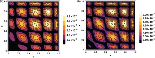
Table 1. MAEs and CO at $\eta =0.65$ and M = N = P for Example 4.1.

	$\alpha =0.00001$		$\alpha =0.5$		$\alpha =1$
M	MAE$(x,y,t)$	CO	MAE$(x,y,t)$	CO	MAE$(x,y,t)$	CO
2	$9.90\times {10}^{-3}$	–	$1.03\times {10}^{-2}$	–	$2.05\times {10}^{-2}$	–
4	$2.01\times {10}^{-4}$	5.62	$1.02\times {10}^{-4}$	6.66	$5.77\times {10}^{-5}$	8.47
6	$1.48\times {10}^{-7}$	17.79	$1.06\times {10}^{-7}$	15.94	$1.48\times {10}^{-7}$	14.71
8	$1.56\times {10}^{-10}$	23.85	$1.00\times {10}^{-10}$	24.20	$8.42\times {10}^{-11}$	25.98

Example 4.2

Consider the following space variable coefficients 2D-TFTE: (40) $\begin{array}{rl}& {}_0^c{\mathcal{D}}_t^v\mathcal{U}+2e^{(x+y)}{}_0^c{\mathcal{D}}_t^{\eta }\mathcal{U}+{\sin }^2(x+y)\mathcal{U}\\ & =(1+x^2)\frac{{\mathrm{\partial }}^2\mathcal{U}}{\mathrm{\partial }{x}^2}+(1+y^2)\frac{{\mathrm{\partial }}^2\mathcal{U}}{\mathrm{\partial }{y}^2}+f(x,y,t),\\ & (x,y,t)\in \mathrm{\Omega }\times \mathrm{\Lambda },\end{array}$(40) where $\mathrm{\Omega }=(0,1)\times (0,1)$ and $\mathrm{\Lambda }=(0,1]$.

The ICs and BCs can be derived from the exact solution $u(x,y,t)=e^{-t}\sinh \left(x\right)\sinh \left(y\right),$ with the source term $\begin{array}{rl}f(x,y,t)& =(t^{2-2\eta }{E}_{1,3-2\eta }(-t)-2e^{(x+y)}{t}^{1-\eta }{E}_{1,2-\eta }(-t)\\ & +({\sin }^2(x+y)-x^2-y^2-2)e^{-t})\\ & \times \sinh \left(x\right)\sinh \left(y\right),\end{array}$ where $E_{m,n}\left(t\right)$ is the two parameter Mittag–Leffler function [45].

The MAEs and CO of Example 4.2 in which the coefficients are mixture of transcendental and polynomial functions of space variables are tabulated for various values of N = M = P in Table 2 with fractional and integer time derivative order. Figure 2 depicts the t-direction curves of the exact and approximate solutions at various fixed points x = y with M = N = P = 7, $\alpha =1$ and v = 0.9 for Example 4.2. It is observed that the obtained results at various orders of the time derivative and various SG parameters produce high accuracy with small increasing of M.

Figure 2. The t-direction curves of the exact $u(x,y,t)$ and approximate $\overline{u}(x,y,t)$ solutions at M = N = P = 7, $\alpha =0.00001$ and v = 0.9 of Example 4.2.

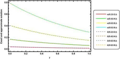
Table 2. MAEs and CO at $v=2\eta$ with M = N = P for Example 4.2.

	$\eta =0.6$		$\eta =0.8$		$\eta =1$
M	MAE$(x,y,t)$	CO	MAE$(x,y,t)$	CO	MAE$(x,y,t)$	CO
2	$2.849\times {10}^{-2}$	–	$2.849\times {10}^{-2}$	–	$2.467\times {10}^{-2}$	–
3	$1.338\times {10}^{-3}$	7.54	$1.338\times {10}^{-3}$	7.54	$1.298\times {10}^{-3}$	7.26
4	$1.458\times {10}^{-4}$	7.71	$1.420\times {10}^{-4}$	7.80	$1.372\times {10}^{-4}$	7.81
5	$3.230\times {10}^{-6}$	17.07	$3.370\times {10}^{-6}$	16.77	$2.955\times {10}^{-6}$	17.20
6	$4.111\times {10}^{-7}$	11.31	$5.721\times {10}^{-7}$	9.73	$1.443\times {10}^{-7}$	16.56

Example 4.3

Consider the following second-order time fractional equation [35–37]: (41) $\begin{array}{rl}& {}_0^c{\mathcal{D}}_t^v\mathcal{U}+B_1(x,y)\frac{\mathrm{\partial }\mathcal{U}}{\mathrm{\partial }t}\\ & =B_3(x,y)\frac{{\mathrm{\partial }}^2\mathcal{U}}{\mathrm{\partial }{x}^2}+B_4(x,y)\frac{{\mathrm{\partial }}^2\mathcal{U}}{\mathrm{\partial }{y}^2}+f(x,y,t),\\ & (x,y,t)\in \mathrm{\Omega }\times \mathrm{\Lambda },\end{array}$(41) where $\mathrm{\Omega }=(0,1)\times (0,1)$ and $\mathrm{\Lambda }=(0,1]$.

The ICs and BCs can be derived from the exact solution $u(x,y,t)=t^{2+\text{β}}\sin \left(x\right)\sin \left(y\right),$ with the source term $\begin{array}{rl}f(x,y,t)& =\left(\frac{\mathrm{\Gamma }(3+\text{β})}{\mathrm{\Gamma }(3+\text{β}-v)}{t}^{2+\text{β}-v}+B_1\right(x,y\left)\right(2+\text{β})t^{1+\text{β}}\\ & +\left(B_3\right(x,y)+B_4(x,y\left)\right)t^{2+\text{β}}\phantom{\frac{\mathrm{\Gamma }(3+\text{β})}{\mathrm{\Gamma }(3+\text{β}-v)}})\sin \left(mx\right)\sin \left(ny\right).\end{array}$ Here, we consider the following four cases of the space variable coefficients:

Case I	[$B_1(x,y)=\cos \left(x+y\right)$, $B_3(x,y)=x^{2}y$ and $B_4(x,y)=x{y}^2$].
Case II	[$B_1(x,y)=\ln \left(1+x+y\right)$, $B_3(x,y)=\sin (1+x^2)$ and $B_4(x,y)=\sin (1+y^2)$ ].
Case III	[$B_1(x,y)=0$, $B_3(x,y)=x^{2}y$ and $B_4(x,y)=x{y}^2$ ].
Case IV	[$B_1(x,y)=0$, $B_3(x,y)=\sin \left(1+x^2\right)$ and $B_4(x,y)=\sin (1+y^2)$ ].

It is notated that Equation (41(41) $\begin{array}{rl}& {}_0^c{\mathcal{D}}_t^v\mathcal{U}+B_1(x,y)\frac{\mathrm{\partial }\mathcal{U}}{\mathrm{\partial }t}\\ & =B_3(x,y)\frac{{\mathrm{\partial }}^2\mathcal{U}}{\mathrm{\partial }{x}^2}+B_4(x,y)\frac{{\mathrm{\partial }}^2\mathcal{U}}{\mathrm{\partial }{y}^2}+f(x,y,t),\\ & (x,y,t)\in \mathrm{\Omega }\times \mathrm{\Lambda },\end{array}$(41) ) with the space coefficient in case I or II represents the 2D-TFDWED, while it represents the 2D-TFWE under the space coefficients of case III or IV. The exact solution is smooth when $\text{β}=2$ and nonsmooth when $1<\text{β}\le 2$.

The MAEs of Example 4.3 with space variable coefficients of cases I-IV for SG parameter $\alpha =0.5$ and time fractional derivative of order v = 1.95 are shown in Table 3 for different values of M = N = P, according to the numerical results, the proposed algorithm offers a high accuracy and rapid convergence at the four cases of the space variable coefficients. Figure 3 depicts the absolute error graphs for cases I and IV of Example 4.3 at M = N = P = 8 with v = 1.65 at time level t = 0.5. Figure 4 depicts the behaviour of approximate solutions for case II of Example 4.3 at various fractional orders of $v=\text{β}$ for $\alpha =1$ and fixed values of y = t = 0.3, 0.7. The exact and approximate solutions of case III of Example 4.3 at $\text{β}=v=1.75$, $\alpha =1$ and x = 0.5 are shown in Figure 5. Table 4 shows RMSEs for two different values of SG parameter ($\alpha =0.00001,0.5$) at M=N=P with the fractional order v = 1.95 of Example 4.3. Also, this table indicates the RMSEs obtained by a hybrid transform-based localized meshless method [36] where $\mathcal{M}$ is the number of evaluation points in the domain Ω with local domain n = 16 for each point. It is clear that the proposed algorithm is more accurate and quickly converges at various values of parameter α. Figures of Example 4.3 are plotted at $\alpha =1$ and M = N = P = 8.

Figure 3. The absolute error surfaces at $\text{β}=2$ and v = 1.65 for t = 0.5 of Example 4.3: (a) Case I and (b) Case IV.

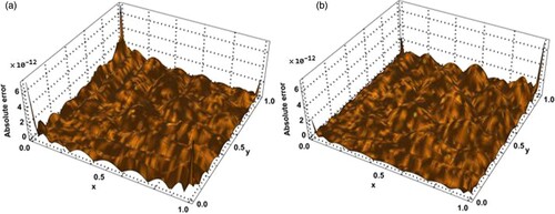
Figure 4. The x-direction curves of the approximate solutions of case II at $\text{β}=v$ of Example 4.3: (a) y = t = 0.3 and (b) y = t = 0.7.

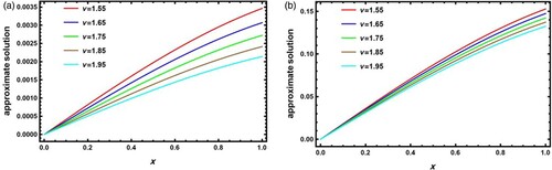
Figure 5. The exact and approximate solutions of case III at $\text{β}=v=1.75$ for x = 0.5 of Example 4.3: (a) Exact solution and (b) Approximate solution.

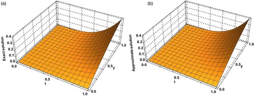
Table 3. Comparison of MAEs at $\alpha =0.5$, $\text{β}=2$ and v = 1.95 of cases I–IV for Example 4.3.

Case	M = 4	M = 5	M = 6	M = 7	M = 8
I	$1.77\times {10}^{-5}$	$1.07\times {10}^{-6}$	$3.18\times {10}^{-8}$	$4.41\times {10}^{-10}$	$5.10\times {10}^{-11}$
II	$2.82\times {10}^{-5}$	$1.01\times {10}^{-6}$	$5.98\times {10}^{-8}$	$1.01\times {10}^{-9}$	$3.69\times {10}^{-11}$
III	$3.77\times {10}^{-5}$	$4.72\times {10}^{-7}$	$7.50\times {10}^{-8}$	$4.61\times {10}^{-10}$	$5.57\times {10}^{-11}$
IV	$3.59\times {10}^{-5}$	$1.03\times {10}^{-6}$	$6.04\times {10}^{-8}$	$1.02\times {10}^{-9}$	$7.18\times {10}^{-11}$

Table 4. Comparison of RMSEs at t = 1, $\text{β}=2$ and v = 1.95 for Example 4.3.

	The proposed method
M	$\alpha =0.00001$	$\alpha =0.5$	$\mathcal{M}$	Uddin et al. [36]
4	$4.90\times {10}^{-4}$	$2.59\times {10}^{-5}$	7	$3.22\times {10}^{-4}$
5	$8.48\times {10}^{-7}$	$5.42\times {10}^{-7}$	10	$1.02\times {10}^{-4}$
6	$4.95\times {10}^{-8}$	$3.24\times {10}^{-8}$	20	$3.97\times {10}^{-5}$
7	$8.07\times {10}^{-10}$	$5.85\times {10}^{-10}$	30	$1.05\times {10}^{-5}$
8	$4.23\times {10}^{-11}$	$3.26\times {10}^{-11}$	40	$1.83\times {10}^{-5}$

5. Conclusion

In the present paper, we have extended and developed a spectral tau algorithm for solving a class of 2D time fractional telegraph equation models with spatial variable coefficients. The existing time fractional mathematical model is characterized as 2D-TFTE or 2D-TFDWED or 2D-TFWE. The algorithm is based on the SG polynomials approximation, the SG operational matrix of fractional differentiation and the tau method. The product of operational matrices of the space vectors is constructed effectively and in a simple way to remove the obstacle that facing the use of the tau method in solving the variable coefficients fractional/integer order PDEs. The proposed algorithm required a small number of basis functions of the SG polynomials to achieve highly accurate approximate solutions because it possess a rapid CO. The proposed algorithm has been tested for the constant and variable coefficients with smooth and non-smooth solutions at various SG parameters α and various fractional derivative orders to ensure the robustness of the algorithm for solving the 2D time fractional telegraph equation models.

Disclosure statement

No potential conflict of interest was reported by the author(s).

References

- Defterli O. Modeling the impact of temperature on fractional order dengue model with vertical transmission. Int J Optim Control Theor Appl. 2020;10:85–93.
- Su N. Fractional calculus for hydrology, soil science and geomechanics. Boca Raton: CRC Press; 2021.
- Herrmann R. Fractional calculus: an introduction for physicists. Hackensack: World Scientific; 2011.
- Obembe AD, Al-Yousef HY, Hossain ME, et al. Fractional derivatives and their applications in reservoir engineering problems. Rev J Pet Sci Eng. 2017;157:312–327.
- Ahmed HF. Analytic approximate solutions for the 1D and 2D nonlinear fractional diffusion equations of Fisher type. Comp rend l'Acadé Bulg des Sci. 2020;73(3):320–330.
- Ahmed HF, Bahgat MSM, Zaki M. Numerical study of multidimensional fractional time and space coupled Burgers' equations. Pramana. 2020;94(1):1–22.
- Oldham KB. Fractional differential equations in electrochemistry. Adv Eng Softw. 2010;41(1):9–12.
- Ara A, Khan NA, Razzaq OA, et al. Wavelets optimization method for evaluation of fractional partial differential equations: an application to financial modelling. Adv Differ Equ. 2018;1:1–13.
- Podlubny I. Fractional differential equations. San Diego: Academic Press; 1999.
- Povstenko Y. Linear fractional diffusion-wave equation for scientists and engineers. New York: Birkhäuser; 2015.
- Povstenko Y. Fractional thermoelasticity. New York: Springer; 2015.
- Kilbas AA, Srivastava HM, Trujillo JJ. Theory and applications of fractional differential equations. Amsterdam: Elsevier; 2006.
- Jajarmi A, Baleanu D. A new fractional analysis on the interaction of HIV with t-cells. Chaos Solitons Fractals. 2018;113:221–229.
- Baleanu D, Jajarmi A, Bonyah E, et al. New aspects of poor nutrition in the life cycle within the fractional calculus. Adv Differ Equ. 2018;2018(1):230–243.
- Ahmed HF, Bahgat MSM, Zaki M. Numerical approaches to system of fractional partial differential equations. J Egypt Math Soc. 2017;25(2):141–150.
- Wang F, Sohail A, Tang Q, et al. Impact of fractals emerging from the fitness activities on the retail of smart wearable devices. Fractals. 2021.
- Sohail A, Yu Z, Arif R, et al. Piecewise differentiation of the fractional order CAR-T cells-SARS-2 virus model. Results Phys. 2022;33:105046.
- Mohyud-Din ST, Nawaz T, Azhar E, et al. Fractional sub-equation method to space–time fractional Calogero–Degasperis and potential Kadomtsev–Petviashvili equations. J Taibah Univ Sci. 2017;11(2):258–263.
- Ahmad S, Ullah A, Akgül A, et al. Numerical analysis of fractional human liver model in fuzzy environment. J Taibah Univ Sci. 2021;15(1):840–851.
- Maiti S, Shaw S, Shit GC. Fractional order model for thermochemical flow of blood with dufour and soret effects under magnetic and vibration environment. Colloids Surf B: Biointerfaces. 2021;197:111395.
- Jordan PM, Puri A. Digital signal propagation in dispersive media. J Appl Phys. 1999;85(3):1273–1282.
- Afrooz K, Abdipour A. Efficient method for time domain analysis of Lossy non uniform multiconductor transmission line driven by modulated signal using FDTD method. IEEE Trans Electromagn Compat. 2012;54(2):482–494.
- Ratner V, Zeevi YY. Denoising enhancing images on elastic manifolds. IEEE Trans Image Process. 2011;20(8):2099–2109.
- Zhang Y, Qian J, Papelis C, et al. Improved understanding of bimolecular reactions in deceptively simple homogeneous media: from laboratory experiments to Lagrangian quantification. Water Resour Res. 2014;50(2):1704–1715.
- Sun HG, Chen W, Li C, et al. Fractional differential models for anomalous diffusion. Phys A: Stat Mech Appl. 2010;389(14):2719–2724.
- Joubert SV, Greeff JC. Accuracy estimates for computer algebra systems initial value problem (IVP)solvers. S Afr J Sci. 2006;102(1):46–50.
- Nigmatullin RR. Realization of the generalized transfer equation in a medium with fractal geometry. Phys Status (B): Basic Res. 1986;133(1):425–430.
- Stefanski TP, Gulgowski J. Signal propagation in electromagnetic media described by fractional-order models. Commun Nonlinear Sci Numer Simul. 2020;82:105029.
- Osman MS. New analytical study of water waves described by coupled fractional variant Boussinesq equation in fluid dynamics. Pramana. 2019;93(2):1–10.
- Mohebbi A, Abbaszadeh M, Dehghan M. The meshless method of radial basis functions for the numerical solution of time fractional telegraph equation. Int J Numer Methods Heat. 2014;24(8):1636–1659.
- Hosseini VR, Shivanian E, Chen W. Local integration of 2-D fractional telegraph equation via local radial point interpolant approximation. Eur Phys J Plus. 2015;130(2):1–21.
- Shivanian E. Spectral meshless radial point interpolation method to two-dimensional fractional telegraph equation. Math Methods Appl Sci. 2016;39(7):1820–1835.
- Hashemi MS, Baleanu D. Numerical approximation of higher-order time-fractional telegraph equation by using a combination of a geometric approach and method of line. J Comput Phys. 2016;316:10–20.
- Ali A, Ali NHM. On skewed grid point iterative method for solving 2D hyperbolic telegraph fractional differential equation. Adv Differ Equ. 2019;2019(1):1–29.
- Hosseini VR, Shivanian E, Chen W. Local radial point interpolation (MLRPI) method for solving time fractional diffusion-wave equation with damping. J Comput Phys. 2016;312:307–332.
- Uddin M, Ali A. A localized transform-based meshless method for solving time fractional wave-diffusion equation. Eng Anal Bound Elem. 2018;92:108–113.
- Kumar A, Bhardwaj A, Kumar BR. A meshless local collocation method for time fractional diffusion wave equation. Comput Math Appl. 2019;78(6):1851–1861.
- Sohail A, Maqbool K, Ellahi R. Stability analysis for fractional-order partial differential equations by means of space spectral time Adams–Bashforth Moulton method. Numer Methods Partial Differ Equ. 2018;34(1):19–29.
- Ahmed HF. Numerical study on factional differential-algebraic systems by means of Chebyshev Pseudo spectral method. J Taibah Uni Sci. 2020;14(1):1023–1032.
- Ahmed HF. A numerical technique for solving multi-dimensional fractional optimal control problems. J Taibah Uni Sci. 2018;12(5):494–505.
- Delkhosh M, Parand K. A new computational method based on fractional Lagrange functions to solve multi-term fractional differential equations. Numer Algor. 2021;88(2):729–766.
- Zaky MA. An accurate spectral collocation method for nonlinear systems of fractional differential equations and related integral equations with nonsmooth solutions. Appl Numer Math. 2020;154:205–222.
- Ahmed HF, Melad MB. A new approach for solving fractional optimal control problems using shifted ultraspherical polynomials. Prog Fract Differ Appl. 2018;4(3):179–195.
- Doman BGS. The classical orthogonal polynomials. New Jersey: World Scientific; 2016.
- Ahmed HF, Moubarak MRA, Hashem WA. Gegenbauer spectral tau algorithm for solving fractional telegraph equation with convergence analysis. Pramana. 2021;95(2):1–16.