On using Shannon entropy measure for formulating new weighted exponential distribution

Abstract

In this article, a new class of weighted exponential distribution called Entropy-Based Exponential weighted distribution (EBEWD) is proposed. The main idea of the new lifetime distribution is in using the Shannon entropy measure as a weighted function. The mathematical properties of the EBEWD, such as reliability measures, moment measures, variability measures, shapes measures, entropy measures and Fisher’s information, were derived. The unknown parameters of the proposed distribution were estimated using the maximum likelihood estimation method. The efficiency and flexibility of the EBEWD were examined numerically and then by a real-life data application. The results revealed that the EBEWD outperforms some existing distributions in terms of their test statistics.

KEYWORDS:

• Exponential distribution
• weighted distribution
• entropy
• distribution theory
• goodness of fit

1. Introduction

The method of weighted distributions as proposed by Fisher’s [1] models of ascertainment on how recorded the probabilities of the events. Weighted distributions are used to select the suitable models for observed data with a technique for fitting models and suitable fits for the data. Rao [2] provides a method of ascertainment concept and how the general formula of weighted distribution is useful for standardizing statistical distributions.

Many researchers start using the concept ofweighted distribution and used the idea of weighted distributions on how effect the original distribution with the new weighted function. Cox [3] suggested using $\text{w}\left(\text{x}\right)=\text{x}$ and calling the new distribution by length-biased weighted distribution. Rao [2] used the weight function $\text{w}\left(\text{x}\right)={\text{x}}^{\delta }$ and proposed the so-called size-biased weighted distribution of order $\delta$. Different weight functions are used in the literature; Table 1 illustrates some of these weight functions with some related references.

Table 1. Improper weight functions.

Weight function w(x)	Related references
$\text{x}$;	Cox [3], Rezzoky and Nadhel [6]; Mir et al. [7]; Mudasir and Ahmad [8].
${\text{x}}^{\delta };\delta >0$;	Rao [2]; Shi et al. [9]; Ye et al. [10]; Das and Roy [11]; Jabeen and Jan [12]
$(1-\text{F}\left(\text{x}\right){)}^{\text{c}};\text{c}>0$	Aleem et al. [13]
$(\text{x}+\alpha {)}^{\text{r}};\alpha \ge 0\text{ and r}\in \text{R}$	Castillo and Casany [14]
${\delta }^{\text{x}};0<\delta <1$	Larose and Dey [15]
$\text{x}\left(\text{x}-1\right)\dots \left(\text{x}+\text{r}-1\right);\text{r}>0$;	Mahfoud and Patil [16]
$\frac{\text{n x}}{\theta };\theta >0,\text{n}>0$;	Al-Kadim and Hussein [17]
$\text{Exp}\left(\delta \mathrm{x}\right)$	Al-Khadim and Hantoosh [18]; Bashir and Rasul [19]; Al-Kadim and Hussein [17]
$\text{Exp}\left(\frac{\text{t}{\text{x}}^2}{2}\right)$	Modi [20]
$(1-\text{Exp}\left(\theta \mathrm{x}\right){)}^{\text{n}};\text{n},\theta >0$	Kharazmi et al. [21]

The main idea of this paper is to introduce a new weight function that is used in quantifying the maximum amount of information in a random variable called entropy [4] to the context of weighted distributions. Accordingly, the article is organized as follows: the next section introduces the new weigh function. The new exponential probability density function is given in Section 3. The statistical measures of the modified exponential distribution are given from Section 3 to Section 10. Parameter estimation is given in Section 11 while in Section 12 the benefit of fitting data to the new distribution model based on a real case study is discussed. The article ends with a concluding remark section.

2. Proposed weighted function

Let X be a random variable with probability density function (pdf) $f\left(x,\theta \right)$ where$\theta$ is an unknown parameter, then the corresponding weighted density function is defined as follows: (1) $g\left(x,\theta \right)=\frac{w\left(x\right)f\left(x,\theta \right)}{E\left[w\left(x\right)\right]}$(1) where $w\left(x\right)$ is a non-negative weighted function; and $E\left[w\left(x\right)\right]$ is the expected value of the weighted function. It is assumed that the expected value of the weighted function exists, and it is positive. The problem in formulating the weighted distribution occurs in selecting a suitable weighted function such that the new distribution is more suitable than the original distribution $f\left(x,\theta \right)$, and provides a better fit for the data than some existing distributions.

The suggested weighted function in this article is entropy, which is defined by Shannon [5] as a negative average of the logarithm of a pdf and called the amount of self-information for a given random variable. Statistically, let X be a continuous random variable with pdf $f\left(x,\theta \right)$, then the entropy is defined as follows: (2) $H\left(x\right)=-{\int }_{-\mathrm{\infty }}^{\mathrm{\infty }}ln\left(f\left(x,\theta \right)\right)f\left(x,\theta \right)dx$(2) Based on (2), the suggested weight function will be $\begin{array}{r}\text{w}\left(\text{x}\right)=-\ln \left(\text{f}\left(\text{x},\theta \right)\right)\end{array}$ Then using this function in (1), we will have the new formulation of the weighted distribution as follows: (3) $g\left(x,\theta \right)=\frac{-\ln \left(f\left(x,\theta \right)\right)f\left(x,\theta \right)}{E\left[-ln\left(f\left(x,\theta \right)\right)\right]}$(3)

3. Entropy-based weighted exponential distribution

The exponential distribution is the most known and used continuous distribution for lifetime data applied in many sciences, such as engineering, economics, medicine, biomedical and in many industrial applications. However, the exponential distribution does not provide a significant fit for some real life-time applications, where the hazard rate function and the mean residual life function of exponential distribution are always constant. Therefore, a more suitable distribution is needed; one of the creative ideas is to form a weighted form of the exponential distribution with a given weight function.

Definition 3.1:

A non-negative continuous random variable X is said to have an exponential distribution if it has a pdf and CDF: (4) $\text{f}\left(\text{x},\lambda \right)=\{\begin{array}{c}\lambda {\text{e}}^{-\lambda \mathrm{x}};\text{ x}\ge 0;\lambda >0\\ 0;\text{otherwise }\end{array}$(4) and (5) $F\left(x,\lambda \right)=\{1-e^{-\lambda x};x\ge 0;\lambda >0$(5) where $\lambda$ is the distribution parameter and called the rate of the distribution. When $\lambda =1$, then the distribution is the standard exponential.

Corollary 3.1:

Let X be a non-negative continuous random variable X with pdf as given in 4, then the entropy is $\begin{array}{r}{\text{H}}_{\text{S}}\left(\text{X}\right)=-\text{E}\left[\text{ln}\left(\text{f}\left(\text{x},\lambda \right)\right)\right]=1-\text{ln}\left(\lambda \right)\end{array}$ This result can be used to develop a new pdf. Therefore, using (1), the entropy-based weighted exponential distribution (EB-WED) will be (6) $\text{g}\left(\text{x},\lambda \right)=\frac{\lambda \mathrm{x}-\ln \left(\lambda \right)}{1-\text{ln}\left(\lambda \right)}\lambda {\text{e}}^{-\lambda \mathrm{x}};\text{ x}>0;\text{ln}\left(\lambda \right)\ne 1$(6) The cumulative distribution function CDF of the EB-WED is (7) $\text{G}\left(\text{x},\lambda \right)={\int }_0^{\text{x}}\text{g}\left(\text{t},\lambda \right)\text{dt }=1-\frac{\left(1+\lambda \mathrm{x}-\text{ln}\left(\lambda \right)\right)}{1-\text{ln}\left(\lambda \right)}{\text{e}}^{-\lambda \mathrm{x}}$(7) Note that, the pdf given in (6) is a non-negative real-valued function, which means $\text{ g}\left(\text{x},\lambda \right)>0$. This is true iff $\begin{array}{r}\frac{\lambda \mathrm{x}-\ln \left(\lambda \right)}{1-\text{ln}\left(\lambda \right)}>0or\lambda {\text{e}}^{-\lambda \mathrm{x}}>0\end{array}$ Based on this fact, some restriction on the pdf range depends on the parameter value. Three cases were obtained as follows:

• if $0<\lambda \le 1$; then $\text{g}\left(\text{x},\lambda \right)>0;\mathrm{\forall }0<\text{ x}<\mathrm{\infty }$

• if $1<\lambda \le {\text{e}}^1$; then $\text{g}\left(\text{x},\lambda \right)>0;\text{if }\frac{\ln \left(\lambda \right)}{\lambda }<x<\mathrm{\infty }$

• if $\lambda >{\text{e}}^1$ ; then $\text{g}\left(\text{x},\lambda \right)>0;\text{if}0<\text{x}<\frac{\ln \left(\lambda \right)}{\lambda }$

For better visualization see Figure 1 the pdf of EB-WEB.

Figure 1. The pdf of EB-WED for different values of $\lambda$.

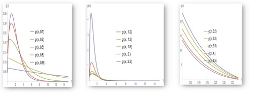
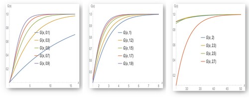
Figure 1 shows that the pdf is skewed to the right. However, when $\lambda$ belongs to the interval $0<\lambda <1$ or $1<\lambda <{\text{e}}^1$, then the pdf has a clear shoulder as $\lambda$ increases. When $\lambda <{\text{e}}^1$ the pdf has shrinkages and does not have a clear shoulder. Moreover, the CDF is given in Figure 2 noting that $\text{G}\left(\text{x},\lambda \right)>0$ must be held. $\begin{array}{r}1-\frac{\left(1+\lambda x-ln\left(\lambda \right)\right)}{1-ln\left(\lambda \right)}{\text{e}}^{-\lambda x}>0\end{array}$

Figure 2. The CDF of EB-WED for different values of $\lambda$.

4. Moments and related measures of the EB-WED

The rth moment of the EB-WED random variable is defined as $\begin{array}{r}{\mu }_r^{\mathrm{\prime }}=E\left(X^r\right)={\int }_{-\mathrm{\infty }}^{\mathrm{\infty }}{x}^{r}g\left(x,\lambda \right)dx\end{array}$ Now, based on three cases the pdf given in (7) the rth moment of X is $\begin{array}{r}E\left(X^r\right)=\{\begin{array}{c}{\displaystyle {\int }_0^{\mathrm{\infty }}{x}^{r}g\left(x,\lambda \right)dx;if0<\lambda \le 1}\\ {\displaystyle {\int }_{\frac{\ln \left(\lambda \right)}{\lambda }}^{\mathrm{\infty }}{x}^{r}g\left(x,\lambda \right)dx;if1<\lambda \le e^1}\\ {\displaystyle {\int }_0^{\frac{\ln \left(\lambda \right)}{\lambda }}{x}^{r}g\left(x,\lambda \right)dx;if\lambda >e^1}\end{array}\end{array}$

Theorem 4.1:

Let X be a random variable following the EB-WED. Then, the rth moment of X is $\begin{array}{r}E\left(X^r\right)=\{\begin{array}{c}A1;if0<\lambda \le 1\\ A1-A2;if1<\lambda \le e^1\\ A2;if\lambda >e^1\end{array}\end{array}$ where $\begin{array}{r}A1=\frac{1}{1-ln\lambda }\left[\frac{\left(r+1\right)!-\left(r\right)!ln\lambda }{{\lambda }^r}\right]\end{array}$ $\begin{array}{r}A2=\frac{\begin{array}{c}\lambda \left\{\mathrm{\Gamma }\left(r+2,ln\left(\lambda \right)\right)-\mathrm{\Gamma }\left(r+2\right)\right\}\\ +ln\left(\lambda \right)\left\{\mathrm{\Gamma }\left(r+1\right)-\mathrm{\Gamma }\left(r+1,ln\left(\lambda \right)\right)\right\}\end{array}}{{\lambda }^r\left(ln\left(\lambda \right)-1\right)}\end{array}$

Proof:

The rth moment of the EB-WED can be obtained using the mathematical expectation: $\begin{array}{rl}E\left(X^r\right)& ={\int }_0^{\mathrm{\infty }}{x}^{r}g\left(x,\lambda \right)dx\end{array}$ $\begin{array}{rl}E\left(X^r\right)& ={\int }_0^{\mathrm{\infty }}{x}^r\frac{\lambda x-\ln \left(\lambda \right)}{1-ln\left(\lambda \right)}\lambda e^{-\lambda x}dx\end{array}$ which can be simplified to $\begin{array}{rl}E\left(X^r\right)& =\frac{1}{1-ln\lambda }[\lambda {\int }_0^{\mathrm{\infty }}{x}^{r+1}\lambda e^{-\lambda x}dx-\ln (\lambda )\\ & \times {\int }_0^{\mathrm{\infty }}{x}^r\lambda e^{-\lambda x}dx]\end{array}$ which can be simplified to $\begin{array}{r}E\left(X^r\right)=\frac{1}{1-ln\lambda }\ast \left[\frac{\left(r+1\right)!-\left(r\right)!ln\lambda }{{\lambda }^r}\right]\end{array}$ End of the proof for case 1.

Now case 3 has $\begin{array}{rl}E\left(X^r\right)& =\frac{1}{1-ln\lambda }[\lambda {\int }_0^{\frac{\ln \left(\lambda \right)}{\lambda }}{x}^{r+1}\lambda e^{-\lambda x}dx\\ & -\ln \left(\lambda \right){\int }_0^{\frac{\ln \left(\lambda \right)}{\lambda }}{x}^r\lambda e^{-\lambda x}dx]\end{array}$ The integration within this expected value can be evaluated easily based on the incomplete gamma function and using the following: $\begin{array}{r}{\int }_0^{\text{a}}{\text{x}}^{\text{r}}\lambda {\text{e}}^{-\lambda \mathrm{x}}\text{dx }=\frac{1}{{\lambda }^{\text{r}}}\left\{\mathrm{\Gamma }\left(\text{r}+1\right)-\mathrm{\Gamma }\left(\text{r}+1,\mathrm{a}\lambda \right)\right\}\end{array}$ Therefore, $\begin{array}{rl}E\left(X^r\right)& =\frac{1}{1-ln\lambda }[\lambda \frac{1}{{\lambda }^r}\left\{\mathrm{\Gamma }\left(r+2\right)-\mathrm{\Gamma }\left(r+2,\frac{\ln \left(\lambda \right)}{\lambda }\lambda \right)\right\}\\ & \times -\ln \left(\lambda \right)\frac{1}{{\lambda }^r}\left\{\mathrm{\Gamma }\left(r+1\right)-\mathrm{\Gamma }\left(r+1,\frac{\ln \left(\lambda \right)}{\lambda }\lambda \right)\right\}\end{array}$ which can be simplified to $\begin{array}{rl}E\left(X^r\right)& =\frac{1}{{\lambda }^r\left(1-ln\lambda \right)}\left[\lambda \right\{\mathrm{\Gamma }\left(r+2\right)-\mathrm{\Gamma }\left(r+2,\ln \left(\lambda \right)\right)\}\\ & -\ln \left(\lambda \right)\left\{\mathrm{\Gamma }\left(r+1\right)-\mathrm{\Gamma }\left(r+1,\ln \left(\lambda \right)\right)\right\}\end{array}$ which ends the proof of case 3. Noting that Case 2 can be obtained directly by finding the differences between case 1 and case 3.

To reduce the number of cases due to the dependence of the variable range on the parameter value, and for the similarities of steps in getting the results, we will consider the results in this article when $0<x<\mathrm{\infty }$.

Theorem 4.2:

Assume that the random variable X follows the EB-WED, then the moment-generating function, ${\text{M}}_{\text{X}\left(\text{EB}-\text{WED}\right)}$ (t), of X is defined as $\begin{array}{r}{M}_X\left(t\right)=\frac{\lambda }{1-ln\lambda }\ast \left[\frac{\left[\lambda -\lambda ln\lambda +tln\lambda \right]}{{\left(\lambda -t\right)}^2}\right]\end{array}$

Proof

The moment-generating function is defined as $\begin{array}{r}{M}_X\left(t\right)=E\left(e^{tX}\right)={\int }_0^{\mathrm{\infty }}{e}^{tx}g\left(x,\lambda \right)dx\end{array}$ Therefore, $\begin{array}{r}{M}_{XEB\mathrm{\_}WED}\left(t\right)={\int }_0^{\mathrm{\infty }}{e}^{tx}\frac{\lambda x-\ln \left(\lambda \right)}{1-ln\left(\lambda \right)}\lambda e^{-\lambda x}dx\end{array}$ This can be simplified to $\begin{array}{r}{M}_{XEB-WED}\left(t\right)=\frac{\lambda }{1-ln\lambda }\ast {\int }_0^{\mathrm{\infty }}\left(\lambda x-\ln \left(\lambda \right)\right)e^{-\left(\lambda -t\right)x}dx\end{array}$ After distributing the terms we have $\begin{array}{rl}{M}_{XEB-WED}\left(t\right)& =\frac{\lambda }{1-ln\lambda }\ast {\int }_0^{\mathrm{\infty }}\lambda x{e}^{-\left(\lambda -t\right)x}dx\\ & -{\int }_0^{\mathrm{\infty }}\ln \left(\lambda \right))e^{-\left(\lambda -t\right)x}dx\end{array}$ Then $\begin{array}{r}{M}_X\left(t\right)=\frac{\lambda }{1-ln\lambda }\ast \left[\frac{\left[\lambda -\lambda ln\lambda +tln\lambda \right]}{{\left(\lambda -t\right)}^2}\right]\end{array}$ This ends the proof.

Theorem 4.3:

The harmonic mean of EB-WED distribution is defined as $\begin{array}{r}{H}_{xEB-WED}=\frac{\lambda }{1-ln\left(\lambda \right)}\left[1-\mathrm{\Gamma }\left(0,\mathrm{\infty }\right)ln\lambda \right];\end{array}$

Proof:

The following integral is used to compute the Harmonic mean $\begin{array}{r}H={\int }_0^{\mathrm{\infty }}\frac{1}{x}g\left(x,\lambda \right)dx\end{array}$ Therefore $\begin{array}{r}H={\int }_0^{\mathrm{\infty }}\frac{1}{x}\ast \frac{\lambda x-\ln \left(\lambda \right)}{1-ln\left(\lambda \right)}\lambda e^{-\lambda x}dx\end{array}$ After rearranging the terms, we have $\begin{array}{r}H=\frac{\lambda }{1-ln\left(\lambda \right)}{\int }_0^{\mathrm{\infty }}\frac{1}{x}\ast \left(\lambda x-\ln \left(\lambda \right)\right)e^{-\lambda x}dx\end{array}$ This can be simplified to $\begin{array}{r}H=\frac{\lambda }{1-ln\left(\lambda \right)}{\int }_0^{\mathrm{\infty }}\frac{1}{x}\left(\lambda x{e}^{-\lambda x}dx\right)-{\int }_0^{\mathrm{\infty }}\frac{1}{x}\ln \left(\lambda \right)e^{-\lambda x}dx\end{array}$ Then $\begin{array}{r}H=\frac{\lambda }{1-ln\left(\lambda \right)}\left[1-ln\lambda {\int }_0^{\mathrm{\infty }}\frac{1}{x}{e}^{-\lambda x}dx\right];\end{array}$ where ${\int }_0^{\mathrm{\infty }}\frac{1}{x}{e}^{-\lambda x}dx=\mathrm{\Gamma }\left(0,\mathrm{\infty }\right)$ This ends the proof.

Theorem 4.4:

The mode of the EB-WED distribution is $\begin{array}{r}{x}_M=\frac{ln\lambda +1}{\lambda }\end{array}$

Proof

The pdf of the EB-WED distribution is $g\left(x,\lambda \right)=\frac{\lambda x-\ln \left(\lambda \right)}{1-ln\left(\lambda \right)}\lambda e^{-\lambda x}$ and its logarithm $\begin{array}{r}\ln \left(g\right(x,\lambda \left)\right)=ln\left[\frac{\lambda x-\ln \left(\lambda \right)}{1-ln\left(\lambda \right)}\lambda e^{-\lambda x}\right]\end{array}$ After rearranging the terms, we have $\begin{array}{r}\ln \left(g\right(x,\lambda \left)\right)=ln\left(\lambda x-\ln \left(\lambda \right)\right)-ln\left(1-ln\left(\lambda \right)\right)+ln\left(\lambda \right)-\lambda x\end{array}$ Finding the first derivative with respect to x, we have $\begin{array}{r}\frac{d}{dx}\ln \left(g\right(x,\lambda \left)\right)=\frac{\lambda }{\lambda x-\ln \left(\lambda \right)}-0+0-\lambda \end{array}$ Setting to zero and solving for x to get $\begin{array}{r}x=\frac{\lambda ln\lambda +\lambda }{{\lambda }^2}\end{array}$ This ends the proof.

5. Measures of variability and distribution shape of the EB-WED

Measures of variability or relative variability can be obtained using the first two moments, based on Theorem 1:

• The mean E(X) of the EB-WED is $\begin{array}{r}\mu =\text{E}\left[\text{X}\right]={\int }_0^{\mathrm{\infty }}\text{x g}\left(\text{x},\lambda \right)\text{dx }=\frac{2-\text{ln}\left(\lambda \right)}{\lambda \left(1-\mathrm{l}\mathrm{n}\lambda \right)},\mathrm{l}\mathrm{n}\lambda \ne 1\end{array}$

• The second moment E(${\text{X}}^2$) of the EB-WED is $\begin{array}{r}\text{E}\left[{\text{X}}^2\right]=\frac{6-2\mathrm{l}\mathrm{n}\lambda }{{\lambda }^2\left(1-\mathrm{l}\mathrm{n}\lambda \right)},\mathrm{l}\mathrm{n}\lambda \ne 1\end{array}$

Then, the population variance is $\begin{array}{r}{\sigma }^2=\text{ E}\left[{\text{X}}^2\right]-(\text{E}\left[\text{X}\right]{)}^2=\frac{2-4\mathrm{l}\mathrm{n}\lambda +{\left(\mathrm{l}\mathrm{n}\lambda \right)}^2}{{\lambda }^2{\left(1-\mathrm{l}\mathrm{n}\lambda \right)}^2},\mathrm{l}\mathrm{n}\lambda \ne 1\end{array}$ Moreover, the coefficient of variation for EB-WED is given by $\begin{array}{r}\text{CV}=\frac{\sigma }{\mu }\end{array}$ which is equivalent to $\begin{array}{r}\text{CV}=\frac{\sqrt{\frac{2-4\mathrm{l}\mathrm{n}\lambda +{\left(\mathrm{l}\mathrm{n}\lambda \right)}^2}{{\lambda }^2{\left(1-\mathrm{l}\mathrm{n}\lambda \right)}^2}}}{\frac{\text{ln}\left(\lambda \right)-2}{\lambda \left(1-\mathrm{l}\mathrm{n}\lambda \right)}}=\frac{\sqrt{2-4\mathrm{l}\mathrm{n}\lambda +{\left(\mathrm{l}\mathrm{n}\lambda \right)}^2}}{\text{ln}\left(\lambda \right)-2},\mathrm{l}\mathrm{n}\lambda \ne 2\end{array}$ The measures of shapes can be obtained based on the third and the fourth moments given by Theorem 1:

• The third moment E(${\text{X}}^3$) of the EB-WED is $\begin{array}{r}\text{E}\left[{\text{X}}^3\right]={\int }_0^{\mathrm{\infty }}{\text{x}}^3\text{g}\left(\text{x},\lambda \right)\text{dx}=\frac{24-6\mathrm{l}\mathrm{n}\lambda }{{\lambda }^3\left(1-\mathrm{l}\mathrm{n}\lambda \right)},\mathrm{l}\mathrm{n}\lambda \ne 1\end{array}$

• The fourth moment E(${\text{X}}^4$) of the EB-WED is $\begin{array}{r}\text{E}\left[{\text{X}}^4\right]={\int }_0^{\mathrm{\infty }}{\text{x}}^4\text{g}\left(\text{x},\lambda \right)\text{dx}=\frac{120-24\mathrm{l}\mathrm{n}\lambda }{{\lambda }^4\left(1-\mathrm{l}\mathrm{n}\lambda \right)},\mathrm{l}\mathrm{n}\lambda \ne 1\end{array}$

Accordingly, Skewness measures symmetry as

$\text{SK}=\frac{\text{E}\left[{\text{X}}^3\right]-3\mu {\sigma }^2-{\mu }^3}{{\sigma }^3}$ is defined as $\begin{array}{rl}& \text{S}{\text{K}}_{\text{EB}-\text{WED}}\\ & =\frac{\left[\begin{array}{c}\left(2-4\mathrm{l}\mathrm{n}\lambda +{\left(\mathrm{l}\mathrm{n}\lambda \right)}^2\right)\left(24-6\mathrm{l}\mathrm{n}\lambda \right){\left(1-\mathrm{l}\mathrm{n}\lambda \right)}^2-\\ \left(6-3\mathrm{l}\mathrm{n}\lambda \right){\left(2-4\mathrm{l}\mathrm{n}\lambda +{\left(\mathrm{l}\mathrm{n}\lambda \right)}^2\right)}^2\end{array}\right]}{{\lambda }^2{\left(1-\mathrm{l}\mathrm{n}\lambda \right)}^2}\end{array}$ Moreover, the coefficient of kurtosis as $\text{Ku}=\frac{\text{E}\left[{\text{x}}^4\right]-4\mu \mathrm{E}\left[{\text{x}}^3\right]+6{\sigma }^2\text{E}\left[{\text{x}}^2\right]-3\text{E}\left[{\text{x}}^4\right]}{{\sigma }^4}$ for EB-WED is defined as $\begin{array}{rl}& \text{K}{\text{u}}_{\text{EB}-\text{WED}}\\ & =\frac{\left[\begin{array}{c}\begin{array}{c}\left(120-24\mathrm{l}\mathrm{n}\lambda \right){\left(1-\mathrm{l}\mathrm{n}\lambda \right)}^3\\ -\left(8-4\mathrm{l}\mathrm{n}\lambda \right)\left(24-6\mathrm{l}\mathrm{n}\lambda \right){\left(1-\mathrm{l}\mathrm{n}\lambda \right)}^2+\end{array}\\ \begin{array}{c}\left(36-12\mathrm{l}\mathrm{n}\lambda \right)\left(2-4\mathrm{l}\mathrm{n}\lambda +{\left(\mathrm{l}\mathrm{n}\lambda \right)}^2\right)\left(1-\mathrm{l}\mathrm{n}\lambda \right)\\ +\left(360-72\mathrm{l}\mathrm{n}\lambda \right){\left(1-\mathrm{l}\mathrm{n}\lambda \right)}^3\end{array}\end{array}\right]}{\frac{{\left(2-4\mathrm{l}\mathrm{n}\lambda +{\left(\mathrm{l}\mathrm{n}\lambda \right)}^2\right)}^8}{{\lambda }^4{\left(1-\mathrm{l}\mathrm{n}\lambda \right)}^4}}\end{array}$ Table 2 gives a numerical illustration of all statistical measures of the EB-WED with different parameter values. The results indicated that the population means values increase as the value of $\lambda$ increases, noting that when $\lambda =1$, then EB-WED is the standard exponential distribution. While the values of the variance, coefficient of variation, skewness and kurtosis decrease as $\lambda$ increases.

Table 2. Numerical values of all statistical measures for the EB-WED.

$\lambda$	${\mu }_{\text{EB}\mathrm{\_}\text{EWD }}$	${{\sigma }^2}_{\text{EB}\mathrm{\_}\text{EWD}}$	$\text{C}{\text{V}}_{\text{EB}\mathrm{\_}\text{EWD}}$	$\text{S}{\text{K}}_{\text{EB}\mathrm{\_}\text{EWD}}$	$\text{K}{\text{U}}_{\text{EB}\mathrm{\_}\text{EWD}}$
0.1	0.00346	1.78351	0.944438	151.39	13.0279
0.2	0.04793	1.71301	0.920046	40.4897	6.91612
0.3	0.21913	1.65522	0.897314	18.9065	4.84575
0.4	0.63997	1.60393	0.87455	11.071	3.8046
0.5	1.46876	1.55728	0.851031	7.32962	3.18123
0.6	2.90761	1.51489	0.826289	5.238	2.76982
0.7	5.225	1.47728	0.799934	3.94057	2.48157
0.8	8.80248	1.44586	0.77158	3.073	2.27196
0.9	14.2292	1.42329	0.740805	2.45792	2.11631
1	22.5	1.41421	0.707106	2	2
1.1	35.4616	1.42690	0.669857	1.64372	1.91396
1.2	56.9269	1.47678	0.628224	1.35436	1.85248
1.3	95.8725	1.59495	0.581044	1.10857	1.81206
1.4	177.561	1.85182	0.526574	0.889211	1.79078
1.5	395.037	2.43711	0.461937	0.682175	1.78799
1.6	1294.97	4.0353	0.381607	0.474053	1.80425
1.7	12431.4	11.2315	0.271419	0.249811	1.84147

6. Measures of reliability

In this section, the Measure of Reliability of the EB-WED distribution is derived.

Corollary 6.1:

Suppose that X is a non-negative continuous random variable that has the pdf and CDF as given in 7 and 8, respectively, then

• The hazard function is $\begin{array}{rl}& \text{H}\left(\text{t},\lambda \right)=\frac{\text{g}\left(\text{t},\lambda \right)}{1-\text{G}\left(\text{t},\lambda \right)}\end{array}$ $\begin{array}{rl}& {\text{H}}_{\text{EB}\mathrm{\_}\text{EWD}}\left(\text{t},\lambda \right)=\frac{(\lambda \mathrm{t}-\ln (\lambda \left)\right)\lambda }{\left(\ln \left(\lambda \right)-1-\lambda \mathrm{t}\right)}\end{array}$

• The reliability functions $\begin{array}{rl}& \text{R}\left(\text{t},\lambda \right)=\text{P}\left(\text{X}>t\right)=1-p\left(X\le t\right)=1-\text{G}\left(\text{t},\lambda \right)\end{array}$ $\begin{array}{rl}& {\text{R}}_{\text{EB}\mathrm{\_}\text{EWD}}\left(\text{t},\lambda \right)=\frac{\left(\ln \left(\lambda \right)-1-\lambda \mathrm{t}\right)}{1-\ln \left(\lambda \right)}{\text{e}}^{-\lambda \mathrm{t}}\end{array}$

• The reversed hazard rate function $\begin{array}{rl}& \text{RH}\left(\text{x},\lambda \right)=\frac{\text{g}\left(\text{x},\lambda \right)}{\text{G}\left(\text{x},\lambda \right)}\end{array}$ $\begin{array}{rl}& \text{R}{\text{H}}_{\text{EB}\mathrm{\_}\text{EWD}}\left(\text{x},\lambda \right)=-\frac{(\lambda \mathrm{x}-\ln (\lambda \left)\right)\lambda }{\begin{array}{l}{\text{e}}^{-\lambda \mathrm{x}}\left(\text{ln}\left(\lambda \right)-1\right)+1\\ +\lambda \mathrm{x}-\text{ln}\left(\lambda \right)\end{array}}\end{array}$

• The odds function $\begin{array}{rl}& \text{O}\left(\text{x},\lambda \right)=\frac{\text{G}\left(\text{x},\lambda \right)}{1-\text{G}\left(\text{x},\lambda \right)}\end{array}$ $\begin{array}{rl}& {\text{O}}_{\text{EB}\mathrm{\_}\text{EWD}}\left(\text{x},\lambda \right)=\frac{\left[\left(\ln \left(\lambda \right)-1\right){\text{e}}^{-\lambda \mathrm{x}}+\lambda \mathrm{x}-\text{ln}\left(\lambda \right)+1\right]}{\left(1-\text{ln}\left(\lambda \right)+\lambda \mathrm{x}\right)}\end{array}$

Figures 3–6 show the behaviour of the EB-WED using its reliability measures.

Figure 3. The hazard function of EB-WED for different values of $\lambda$.

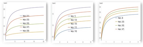
Figure 4. The reliability function of EB-WED for different values of $\lambda$.

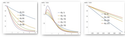
Figure 5. The reversed hazard function of EB-WED for different values of $\lambda$.

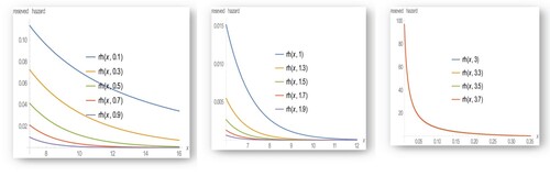
Figure 6. The odd function of EB-WED for different values of $\lambda$.

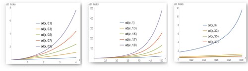
The above figures indicate that as $\lambda$ increases the hazard rate function and the odd function increases while it decreases with the other reliability measures.

7. Stochastic orderings

Let X and Y be two continuous random variables with probability density functions ${\text{f}}_{\text{x}}\left(\text{x}\right)$ and ${\text{f}}_{\text{y}}\left(\text{x}\right)$, and the associated cumulative distributions functions are ${\text{F}}_{\text{x}}\left(\text{x}\right),\text{and }{\text{F}}_{\text{y}}\left(\text{x}\right)$, then

• Stochastic order $\text{X}{\le }_{\text{st }}\text{Y}$ if ${\text{F}}_{\text{x}}\left(\text{x}\right){\ge }_{\text{st }}{\text{F}}_{\text{y}}\left(\text{x}\right)$ for all x;

• Hazard rate order $\text{X}{\le }_{\text{hr }}\text{Y}$ if ${\text{h}}_{\text{x}}\left(\text{x}\right){\ge }_{\text{hr }}{\text{h}}_{\text{y}}\left(\text{x}\right)$ for all x;

• Mean residual life order $\text{ X}{\le }_{\text{mr }}\text{Y}$ if ${\text{m}}_{\text{x}}\left(\text{x}\right){\le }_{\text{mr }}{\text{m}}_{\text{y}}\left(\text{x}\right)$ for all x;

• Likelihood ratio order $\text{X}{\le }_{\text{lr }}\text{Y}$ if $\frac{{\text{f}}_{\text{x}}\left(\text{x}\right)}{{\text{f}}_{\text{y}}\left(\text{x}\right)}$ decreases in x.

Thus, $\begin{array}{r}\text{X}{\le }_{\text{lr }}\text{Y}\Rightarrow \text{ X}{\le }_{\text{hr }}\text{Y }\Rightarrow \text{ X}{\le }_{\text{mr }}\text{Y}\end{array}$ $\begin{array}{r}{\downarrow }_{\text{X}{\le }_{\text{st }}\text{Y}}\end{array}$

Theorem 7.1:

Let $\text{X}\sim \text{WB}-\text{WED}\left({\lambda }_1\right)$ and $\text{Y}\sim \text{WB}-\text{WED}\left({\lambda }_2\right)$ and corresponding distribution functions ${\text{F}}_{\text{x}}\left(\text{x}\right)$ and ${\text{F}}_{\text{y}}\left(\text{x}\right)$. If ${\lambda }_1>{\lambda }_2$ then $\text{X}{\le }_{\text{lr }}\text{Y}$ and $\text{ X}{\le }_{\text{hr }}\text{Y}$,$\text{ X}{\le }_{\text{mr }}\text{Y}$ and $\text{X}{\le }_{\text{st }}\text{Y}$

Proof:

• Stochastic order: needs to show that ${\text{F}}_{\text{x}}\left(\text{x}\right){\ge }_{\text{st }}{\text{F}}_{\text{y}}\left(\text{x}\right)$ for all x

For ${\lambda }_1>{\lambda }_2$ then $\begin{array}{r}\frac{\left(1+{\lambda }_1-\ln \left({\lambda }_1\right)\right)}{1-\ln \left({\lambda }_1\right)}{\text{e}}^{-{\lambda }_1\text{x}}\ge \frac{\left(1+{\lambda }_2-\ln \left({\lambda }_2\right)\right)}{1-\ln \left({\lambda }_2\right)}{\text{e}}^{-{\lambda }_2\text{x}}\end{array}$ ${\text{F}}_{\text{x}}\left(\text{x}\right){\ge }_{\text{st }}{\text{F}}_{\text{y}}\left(\text{x}\right)$ For all x, then X is stochastically smaller than Y based on stochastic order $\text{X}{\le }_{\text{st }}\text{Y}$

• Hazard rate order: needs to show that ${\text{h}}_{\text{x}}\left(\text{x}\right){\ge }_{\text{hr }}{\text{h}}_{\text{y}}\left(\text{x}\right)$ for all x

For ${\lambda }_1>{\lambda }_2$ then $\begin{array}{r}\frac{({\lambda }_1\text{t}-\ln ({\lambda }_1\left)\right){\lambda }_1}{\left(\ln \left({\lambda }_1\right)-1-{\lambda }_1\text{x}\right)}\ge \frac{({\lambda }_2\text{t}-\ln ({\lambda }_2\left)\right){\lambda }_2}{\left(\ln \left({\lambda }_2\right)-1-{\lambda }_2\text{x}\right)}\end{array}$ ${\text{h}}_{\text{x}}\left(\text{x}\right){\ge }_{\text{hr }}{\text{h}}_{\text{y}}\left(\text{x}\right)$ For all x, then X is smaller in the hazard rate ordering than Y-based hazard rate order $\text{ X}{\le }_{\text{hr }}\text{Y}$

• Mean residual life order: needs to show that ${\text{m}}_{\text{x}}\left(\text{x}\right){\le }_{\text{mr }}{\text{m}}_{\text{y}}\left(\text{x}\right)$ for all x

For ${\lambda }_1>{\lambda }_2$ then $\begin{array}{r}{\text{m}}_{\text{x}}\left(\text{x}\right)={\int }_{\text{x}}^{\mathrm{\infty }}1-{\text{F}}_{\text{x}}\left(\text{t}\right)\text{ dt };{\text{m}}_{\text{y}}\left(\text{x}\right)={\int }_{\text{x}}^{\mathrm{\infty }}1-{\text{F}}_{\text{y}}\left(\text{t}\right)\text{ dt}\end{array}$ $\begin{array}{r}\frac{{\text{m}}_{\text{x}}\left(\text{x}\right)}{{\text{m}}_{\text{y}}\left(\text{x}\right)}=\frac{\frac{\left(1+{\lambda }_1-\ln \left({\lambda }_1\right)\right)}{1-\ln \left({\lambda }_1\right)}}{\frac{\left(1+{\lambda }_2-\ln \left({\lambda }_2\right)\right)}{1-\ln \left({\lambda }_2\right)}}{\text{e}}^{({\lambda }_2-{\lambda }_1)\text{x}},\text{x}>0;\text{increases in x}\end{array}$ ${\text{m}}_{\text{x}}\left(\text{x}\right){\le }_{\text{mr }}{\text{m}}_{\text{y}}\left(\text{x}\right)$ For all x, then $\text{X}$ is smaller in the mean residual life order than $\text{Y}$-based mean residual life order $\text{ X}{\le }_{\text{mr }}\text{Y}$.

• Likelihood ratio order: needs to show that $\frac{{\text{f}}_{\text{x}}\left(\text{x}\right)}{{\text{f}}_{\text{y}}\left(\text{x}\right)}$ is a decreasing function of x $\begin{array}{r}\frac{f_x\left(x\right)}{f_y\left(x\right)}=\frac{\left[\frac{{\lambda }_{1}x-\ln \left({\lambda }_1\right)}{1-ln\left({\lambda }_1\right)}{\lambda }_1\right]}{\left[\frac{{\lambda }_{2}x-\ln \left({\lambda }_2\right)}{1-ln\left(2\right)}{\lambda }_2\right]}{e}^{({\lambda }_2-{\lambda }_1)x},x>0\end{array}$

Now for ${\lambda }_1>{\lambda }_2$ $\begin{array}{r}\frac{d}{dx}\frac{f_x\left(x\right)}{f_y\left(x\right)}=\frac{\left[\begin{array}{l}{\lambda }_1\left(\ln {\lambda }_2-1\right)e^{({\lambda }_2-{\lambda }_1)x}\\ \left[\begin{array}{c}\left({\lambda }_1{\lambda }_2^2-{\lambda }_1^2{\lambda }_2\right)x^2\\ +\left(\right({\lambda }_1^2-{\lambda }_1{\lambda }_2)ln{\lambda }_2-{\lambda }_2^{2}ln{\lambda }_1\\ +{\lambda }_1{\lambda }_{2}ln{\lambda }_1)x\\ +({\lambda }_{2}ln{\lambda }_1-{\lambda }_{1}ln{\lambda }_1-{\lambda }_1)ln{\lambda }_2\\ +{\lambda }_{2}ln{\lambda }_1\end{array}\right]\end{array}\right]}{\left(ln{\lambda }_1-1\right){\lambda }_2{\left(x{\lambda }_2-ln{\lambda }_2\right)}^2}\end{array}$ $\begin{array}{r},\text{x}<0\end{array}$ X is smaller than Y, $\frac{f_x\left(x\right)}{f_y\left(x\right)}$ decreases in x, then Y is stochastically greater than X based on likelihood ratio order.

8. Information measures

The information measure of the EB-WED random variable is derived as follows:

Theorem 8.1:

Let X be a continuous random variable that has EB-WED distribution, then the Rényi entropy of X is defined as $\begin{array}{rl}{H}_R\left(X\right)& =\frac{1}{1-\alpha }\ln \{{\left(\frac{{\lambda }^2}{1-ln\left(\lambda \right)}\right)}^{\alpha }\\ & \times \left(\frac{1-{\alpha }^{\alpha +1}}{{\alpha }^{\alpha }}\mathrm{\Gamma }\left(\alpha \right)+\mathrm{\Gamma }\left(\alpha +1,-\alpha ln\left(\lambda \right)\right)\right)\}\end{array}$

Proof

Using the Rényi entropy as defined by Rényi [22]

${\text{H}}_{\text{R}}\left(\text{X}\right)=\text{RE}\left(\alpha \right)=\frac{1}{1-\alpha }\text{ ln}{\int }_{-\mathrm{\infty }}^{\mathrm{\infty }}\text{g}(\text{x},\lambda {)}^{\alpha }\text{dx };\alpha \in \left(0,1\right)$,then we have $\begin{array}{r}{H}_R\left(X\right)=\frac{1}{1-\alpha }\ln {\int }_0^{\mathrm{\infty }}{\left(\frac{\lambda x-\ln \left(\lambda \right)}{1-ln\left(\lambda \right)}\lambda e^{-\lambda x}\right)}^{\alpha }dx;\alpha \in \left(0,1\right)\end{array}$ which can be simplified to $\begin{array}{rl}& H_R\left(X\right)=\frac{1}{1-\alpha }\ln {\int }_0^{\mathrm{\infty }}{\left(\frac{\lambda x-\ln \left(\lambda \right)}{1-ln\left(\lambda \right)}\right)}^{\alpha }{\lambda }^{\alpha }{e}^{-\alpha \lambda x}dx\end{array}$ $\begin{array}{rl}{H}_R\left(X\right)& =\frac{1}{1-\alpha }\ln {\int }_0^{\mathrm{\infty }}(\lambda x-\ln \left(\lambda \right){)}^{\alpha }\\ & \times {\left(\frac{\lambda }{1-ln\left(\lambda \right)}\right)}^{\alpha }{e}^{-\alpha \lambda x}dx\end{array}$ After rearranging the terms, $\begin{array}{rl}{H}_R\left(X\right)& =\frac{1}{1-\alpha }\ln \{{\left(\frac{\lambda }{1-ln\left(\lambda \right)}\right)}^{\alpha }\\ & \times {\int }_0^{\mathrm{\infty }}{\left(\lambda x-\ln \left(\lambda \right)\right)}^{\alpha }{e}^{-\alpha \lambda x}dx\}\end{array}$ Now if assume that $\text{ u}=\lambda \mathrm{x}-\ln \left(\lambda \right)$, then du = $\lambda$ dx

Replace x with u, then the integral will be $\begin{array}{rl}{H}_R\left(X\right)& =\frac{1}{1-\alpha }\ln \{{\left(\frac{\lambda }{1-ln\left(\lambda \right)}\right)}^{\alpha }\\ & \times {\int }_{-ln\left(\lambda \right)}^{\mathrm{\infty }}{\left(u\right)}^{\alpha }{e}^{-\alpha \left(u+ln\left(\lambda \right)\right)}\frac{du}{\lambda }\}\end{array}$ $\begin{array}{rl}\left[H_R\right(X)& =\frac{1}{1-\alpha }\ln \{{\left(\frac{\lambda }{1-ln\left(\lambda \right)}\right)}^{\alpha }\frac{e^{-\alpha ln\left(\lambda \right)}}{\lambda }\\ & \times {\int }_{-ln\left(\lambda \right)}^{\mathrm{\infty }}{\left(u\right)}^{\alpha }{e}^{-\alpha u}du\}\end{array}$ which can be simplified to $\begin{array}{rl}{H}_R\left(X\right)& =\frac{1}{1-\alpha }\ln \{{\left(\frac{\lambda }{1-ln\left(\lambda \right)}\right)}^{\alpha }{\lambda }^{-\left(\alpha +1\right)}\\ & \times {\int }_{-ln\left(\lambda \right)}^{\mathrm{\infty }}{\left(u\right)}^{\alpha }{e}^{-\alpha u}du\}\end{array}$ Using integral on gamma function, we have $\begin{array}{rl}{H}_R\left(X\right)& =\frac{1}{1-\alpha }\ln \left\{{\left(\frac{1}{1-ln\left(\lambda \right)}\right)}^{\alpha }\frac{1}{\lambda }\right({\alpha }^{-\alpha }\mathrm{\Gamma }\left(\alpha \right)\\ & +\mathrm{\Gamma }\left(\alpha +1,-\alpha ln\left(\lambda \right)\right)-\alpha \mathrm{\Gamma }\left(\alpha \right)\left)\right\}\end{array}$ After rearranging the terms $\begin{array}{rl}{H}_R\left(X\right)& =\frac{1}{1-\alpha }\ln \{{\left(\frac{1}{1-ln\left(\lambda \right)}\right)}^{\alpha }\\ & \times \frac{1}{\lambda }\left(\frac{1-{\alpha }^{\alpha +1}}{{\alpha }^{\alpha }}\mathrm{\Gamma }\left(\alpha \right)+\mathrm{\Gamma }\left(\alpha +1,-\alpha ln\left(\lambda \right)\right)\right)\}\end{array}$ This ends the proof.

Theorem 8.2:

Let X be a continuous random variable that has EB-WED distribution, then the Shannon entropy of X is defined as follows: $\begin{array}{r}{H}_S\left(X\right)=\lambda E\left(X\right)-\ln \left(\lambda \right)-E\left(\ln \left(\frac{\lambda x-\ln \left(\lambda \right)}{1-ln\left(\lambda \right)}\right)\right)\end{array}$ $\begin{array}{rl}{H}_S\left(X\right)& =\lambda \frac{2-ln\left(\lambda \right)}{\lambda \left(1-ln\lambda \right)}-\ln \left(\lambda \right)-\left\{\frac{\lambda }{1-ln\left(\lambda \right)}\right\{\lambda \left(\right(\ln \left(\lambda \right)\\ & -1\left)ln\right[-\ln \left(\lambda \right)]-1)+LogIntegral\left(\lambda \right)\left\}\right\}\end{array}$

Proof

Using Shannon entropy ${\text{H}}_{\text{S}}\left(\text{X}\right)=-{\int }_{-\mathrm{\infty }}^{\mathrm{\infty }}\text{g}\left(\text{x},\lambda \right)\ln \left(\text{g}\left(\text{x},\lambda \right)\right)\text{dx}$, then the Shannon entropy of EB-WED can be written in terms of integration: $\begin{array}{rl}{H}_S\left(X\right)& =-\int \frac{\lambda x-\ln \left(\lambda \right)}{1-ln\left(\lambda \right)}\lambda e^{-\lambda x}\ln \left(\frac{\lambda x-\ln \left(\lambda \right)}{1-ln\left(\lambda \right)}\lambda e^{-\lambda x}\right)dx\end{array}$ Then using the properties of the ln function, we have $\begin{array}{rl}{H}_S\left(X\right)& =-\int \frac{\lambda x-\ln \left(\lambda \right)}{1-ln\left(\lambda \right)}\lambda e^{-\lambda x}\{\ln \left(\frac{\lambda x-\ln \left(\lambda \right)}{1-ln\left(\lambda \right)}\right)\\ & +\ln \left(\lambda \right)-\lambda x\}dx\end{array}$ This is can be written in terms of expected value: $\begin{array}{r}{H}_S\left(X\right)=\lambda E\left(X\right)-\ln \left(\lambda \right)-E\left(\ln \left(\frac{\lambda x-\ln \left(\lambda \right)}{1-ln\left(\lambda \right)}\right)\right)\end{array}$ where

• E(X) = $\frac{2-ln\left(\lambda \right)}{\lambda \left(1-ln\lambda \right)}$;

• $E(\ln \left(\frac{\lambda x-\ln \left(\lambda \right)}{1-ln\left(\lambda \right)}\right)=E\{\ln \left(\lambda x-\ln \left(\lambda \right)\right)\}-ln(1-ln\left(\lambda \right)$;

and

• $E\left\{\ln \left(\lambda x-\ln \left(\lambda \right)\right)\right\}=\int \frac{\lambda x-\ln \left(\lambda \right)}{1-ln\left(\lambda \right)}\lambda e^{-\lambda x}\ln \left(\lambda x-\ln \left(\lambda \right)\right)dx$

which can be obtained by setting u = $\lambda \mathrm{x}-\ln \left(\lambda \right)$ then $\text{du }=\lambda \mathrm{d}\mathrm{x}$

Therefore $\begin{array}{r}E\left\{\ln \left(\lambda x-\ln \left(\lambda \right)\right)\right\}=\int \frac{uln\left(u\right)}{1-ln\left(\lambda \right)}{e}^{-\left(u+\ln \left(\lambda \right)\right)}du\end{array}$ which is equivalent to $\begin{array}{rl}& \frac{\lambda }{1-ln\left(\lambda \right)}\left\{\lambda \right(\left(\ln \left(\lambda \right)-1\right)ln\left[-\ln \left(\lambda \right)\right]-1)\\ & +LogIntegral\left(\lambda \right)\}\end{array}$ Noting that $\text{ LogIntegral}\left[\lambda \right]$ is the logarithmic integral function that is defined by $\text{LogIntegral}\left(\lambda \right)={\int }_0^{\lambda }\frac{1}{\text{ln}\left(\text{t}\right)}\text{ dt}$

This ends the proof.

9. Extreme order statistics

In this section, the pdf of the minimum and the maximum order statistic of the EB-WED is given. Let X_(1:n), X_(2:n), … , X_(n:n) denote the order statistics of a random sample of size n; X₁, X₂ … , X_n; from a continuous population with pdf $\text{g}\left(\text{x},\lambda \right)$ and CDF $\text{G}\left(\text{x},\lambda \right)$, then the pdf of the ith order statistic X_(i:n) is defined as follows: $\begin{array}{rl}{f}_{\left(i:n\right)}\left(x,\lambda \right)& =\frac{n!}{\left(i-1\right)!\left(n-i\right)!}\\ & \times G(x,\lambda {)}^{i-1}[1-G\left(x,\lambda \right){]}^{n-i}g\left(x,\lambda \right)\end{array}$ Using 7 and 8 will be derived; the pdf of the minimum and the maximum order statistic will be $\begin{array}{rl}{f}_{\left(1:n\right)}\left(x\right)& =n[1-G\left(x\right){]}^{n-1}g\left(x\right)\end{array}$ $\begin{array}{rl}{f}_{\left(1:n\right)}\left(x\right)& =\frac{\left[n\lambda \left(\lambda x-ln\lambda \right){\left(\frac{\left(1+\lambda x-\ln \left(\lambda \right)\right)}{1-\ln \left(\lambda \right)}\right)}^n{e}^{-n\lambda x}\right]}{1+\lambda x-\ln \left(\lambda \right)}\end{array}$ $\begin{array}{rl}{f}_{\left(n:n\right)}\left(x\right)& =n[G\left(x\right){]}^{n-1}g\left(x\right)\end{array}$ $\begin{array}{rl}{f}_{\left(n:n\right)}\left(x\right)& =n{\left[1+\frac{\left(1+\lambda x-\ln \left(\lambda \right)\right)}{\ln \left(\lambda \right)-1}{\text{e}}^{-\lambda x}\right]}^{n-1}\\ & \times \frac{\lambda x-\ln \left(\lambda \right)}{1-ln\left(\lambda \right)}\lambda e^{-\lambda x}\end{array}$

10. Fisher’s information

Derive Fisher’s information of the EB-WED random variable based on $\begin{array}{r}I\left(\lambda \right)=-E\left(\frac{d^2}{d{\lambda }^2}\ln \left(g\left(x,\lambda \right)\right)\right)\end{array}$

Theorem 10.1:

Let X follow the EB-WED distribution, and then its Fisher’s information, FIEB-WED (λ) is $\begin{array}{rl}I\left(\lambda \right)& =\frac{1}{{\lambda }^2}\{1+\frac{1}{\left(1-ln\left(\lambda \right)\right)}-\frac{1}{{\left(1-ln\left(\lambda \right)\right)}^2}\\ & -\left[\frac{\ln \left(\lambda \right)-1}{-\ln {\left(\lambda \right)}^2+2\ln \left(\lambda \right)-2}\right]\\ & +\left[\frac{1+2\left(\ln \left(\lambda \right)-3\right)-2{\lambda }^2\left(\ln \left(\lambda \right)-2\right)}{6\left(\ln \left(\lambda \right)-1\right)}\right]\}\end{array}$

Proof

Fisher’s information is defined as $\begin{array}{r}I\left(\lambda \right)=-E\left(\frac{d^2}{d{\lambda }^2}\ln \left(g\left(x,\lambda \right)\right)\right)\end{array}$ Now, the log of the pdf of the EB-WED is $\begin{array}{rl}\ln \left(g\right(x,\lambda \left)\right)& =ln\left[\frac{\lambda x-\ln \left(\lambda \right)}{1-ln\left(\lambda \right)}\lambda e^{-\lambda x}\right]\end{array}$ $\begin{array}{rl}\ln \left(g\right(x,\lambda \left)\right)& =ln\left[\right(\lambda x)-\ln (\lambda \left)\right]-ln\left[\right(1-ln\left(\lambda \right)]\\ & +ln\left(\lambda \right)-\lambda x\end{array}$ By differentiating the last equation with respect to $\lambda$, then $\begin{array}{r}\frac{dln\left(g\left(x,\lambda \right)\right)}{d\lambda }=\frac{x-\frac{1}{\lambda }}{\lambda x-\ln \left(\lambda \right)}+\frac{1}{\lambda \left(1-ln\left(\lambda \right)\right)}+\frac{1}{\lambda }-x\end{array}$ The second differentiation is $\begin{array}{rl}\frac{d^{2}log\left(g\left(x,\lambda \right)\right)}{d{\lambda }^2}& =\frac{1}{{\lambda }^2\left(\lambda x-\ln \left(\lambda \right)\right)}-\frac{{\left(x-\frac{1}{\lambda }\right)}^2}{{\left(\lambda x-\ln \left(\lambda \right)\right)}^2}\\ & -\frac{1}{{\lambda }^2\left(1-ln\left(\lambda \right)\right)}\\ & +\frac{1}{{\lambda }^2{\left(1-ln\left(\lambda \right)\right)}^2}-\frac{1}{{\lambda }^2}\end{array}$ Now $\begin{array}{rl}I\left(\lambda \right)& =-E\left(\frac{d^2}{d{\lambda }^2}\ln \left(g\left(x,\lambda \right)\right)\right)\end{array}$ $\begin{array}{rl}I\left(\lambda \right)& =-E[\frac{1}{{\lambda }^2\left(\lambda x-\ln \left(\lambda \right)\right)}-\frac{{\left(x-\frac{1}{\lambda }\right)}^2}{{\left(\lambda x-\ln \left(\lambda \right)\right)}^2}\\ & -\frac{1}{{\lambda }^2\left(1-ln\left(\lambda \right)\right)}+\frac{1}{{\lambda }^2{\left(1-ln\left(\lambda \right)\right)}^2}-\frac{1}{{\lambda }^2}]\end{array}$ $\begin{array}{rl}I\left(\lambda \right)& =\frac{1}{{\lambda }^2\left(1-ln\left(\lambda \right)\right)}-\frac{1}{{\lambda }^2{\left(1-ln\left(\lambda \right)\right)}^2}+\frac{1}{{\lambda }^2}\\ & -\frac{1}{{\lambda }^2}E\left[\frac{1}{\left(\lambda x-\ln \left(\lambda \right)\right)}\right]+E\left[\frac{{\left(x-\frac{1}{\lambda }\right)}^2}{{\left(\lambda x-\ln \left(\lambda \right)\right)}^2}\right]\end{array}$ $\begin{array}{rl}I\left(\lambda \right)& =\frac{1}{{\lambda }^2\left(1-ln\left(\lambda \right)\right)}-\frac{1}{{\lambda }^2{\left(1-ln\left(\lambda \right)\right)}^2}+\frac{1}{{\lambda }^2}\\ & -\frac{1}{{\lambda }^2}\left[\frac{1}{-\ln \left(\lambda \right)+\frac{\ln \left(\lambda \right)-2}{\ln \left(\lambda \right)-1}}\right]\\ & +E\left[\frac{x^2-2x\lambda +{\left(\frac{1}{\lambda }\right)}^2}{{\lambda }^2{x}^2-2x\lambda ln\left(\lambda \right)-\ln {\left(\lambda \right)}^2}\right]\end{array}$ $\begin{array}{rl}I\left(\lambda \right)& =\frac{1}{{\lambda }^2}\{1+\frac{1}{\left(1-ln\left(\lambda \right)\right)}-\frac{1}{{\left(1-ln\left(\lambda \right)\right)}^2}\\ & -\left[\frac{\ln \left(\lambda \right)-1}{-\ln {\left(\lambda \right)}^2+2\ln \left(\lambda \right)-2}\right]\\ & +\left[\frac{1+2\left(\ln \left(\lambda \right)-3\right)-2{\lambda }^2\left(\ln \left(\lambda \right)-2\right)}{6\left(\ln \left(\lambda \right)-1\right)}\right]\}\end{array}$

This ends the proof.

Table 3 provides some value of Fisher’s information for EB-WED when λ = 0.1, 0.2, … , 1.3. The results indicated that as $\lambda$ increases as $\text{I}\left(\lambda \right)$ decreases, hence the data provide a lot of “information” about λ

Table 3. Fisher’s information values of the EB-WED for λ value.

$\lambda$	$\text{I}$ ($\lambda$)
0.1	122.212
0.2	33.0092
0.3	15.4564
0.4	8.97248
0.5	5.8077
0.6	3.99245
0.7	2.83383
0.8	2.03493
0.9	1.45005
1	1
1.1	0.637946
1.2	0.333962
1.3	0.067288

11. Parameter estimation

In this section, we use the maximum likelihood estimation method to find a point estimator of the unknown parameter in the EB-WED. Suppose that ${\text{X}}_1,{\text{X}}_2,\dots ,{\text{X}}_{\text{n}}$ is a random sample of size n (independent and identically distributed) following the EB-WED, as given in 7. Using MLE, then the likelihood function is given as follows: $\begin{array}{r}{L}_{EB-WED}\left(\lambda \right)=\prod _{i=1}^n\frac{\lambda x_i-\ln \left(\lambda \right)}{1-ln\left(\lambda \right)}\lambda e^{-\lambda x_i}\end{array}$ which is equivalent to $\begin{array}{r}{L}_{EB-EWD}\left(\lambda \right)=\frac{\lambda }{1-ln\left(\lambda \right)}\prod _1^n\left[\lambda x-\ln \left(\lambda \right)\right]e^{-\lambda x}\end{array}$ Finding the logarithm of the likelihood function $\begin{array}{rl}\ln L_{EB-EWD}\left(\lambda \right)& =\ln \left[\frac{\lambda }{1-ln\left(\lambda \right)}\right]\\ & +\sum _1^n\left[ln\left[\lambda x_i-\ln \left(\lambda \right)\right]\right]-\lambda \sum _1^n{x}_i\end{array}$ By differentiating with respect to$\lambda$ $\begin{array}{rl}\frac{d\ln L_{E{B}_{EWD}}\left(\lambda \right)}{d\lambda }& =\frac{\ln \left(\lambda \right)-2}{\lambda \left(1-ln\left(\lambda \right)\right)}\\ & +\sum _1^n\frac{x_i-\frac{1}{\lambda }}{\lambda x_i-ln\left(x_i\right)}-\sum _1^n{x}_i\end{array}$ The maximum likelihood $\hat{\lambda }$ of $\lambda$ is obtained by equating the above equation to zero. Since the equation is complicated, the point estimator can be found by employing a numerical method to find the point estimator numerically under the following condition: $\begin{array}{r}\frac{{\text{d}}^2\ln {\text{L}}_{\text{E}{\text{B}}_{\text{WED}}}\left(\lambda \right)}{\text{d}{\lambda }^2}<0\end{array}$

12. Application

In this section, real data analysis will be considered to study the performance of the new distributions. Then a comparison will be made with some fitted lifetime distributions: The Marshall Olkin Esscher transformed Laplace distribution, Lindley distribution and exponential distribution.

• The one-parameter Marshall – Olkin Esscher transformed Laplace distribution (MOETLD) was provided by George and George [23] with pdf $\begin{array}{r}f\left(x\right)=\frac{\phi }{1+{\phi }^2}\{\begin{array}{c}{e}^{\phi x},x\le 0\\ e^{-\phi x},x\ge 0\end{array}\end{array}$

• Lindley distribution was provided by Lindley [24] with pdf $\begin{array}{r}f\left(x\right)=\frac{{\theta }^2}{\left(1+\theta \right)}\left(1+x\right)e^{-\theta x};x>0,\theta >0\end{array}$

12.1. Goodness of fit measures

Maydeu et al [25]. The goodness of fit is some of the statistical model for summarize the fit of observation, and how perform model comparisons, where in there mathematical formulas have $\gamma$ the value of the log-likelihood function k is the number of estimated parameters and n is the sample size.

(I) Information Criterion Measures:

• Bayesian Information Criterion (BIC), Schwarz [26]:

It is a statistical measure used to compare between the performances of a set of models, the lower the value the better the model. $\begin{array}{r}BIC=-2\gamma +2kln\left(n\right)\end{array}$

• Akaike Information Criterion (AIC), Akaike [27]:

How well the data are explained by the model suitability and complexity of the model, and the performance of a model is predicted by minimizing the function. The lower the value, the better the model. $\begin{array}{r}AIC=-2\gamma +2k\end{array}$

• Consistent Akaike Information Criterion (CAIC), Bozdogan [28]:

It is a model selection criteria provide an asymptotically how will the model fit the data, and give unbaised estimate of the order of the true model. The model with more parameters fits better than the model that has fewer parameters $\begin{array}{r}CAIC=-2Ln\left(\gamma \right)+k\left(ln\left(n\right)+1\right)\end{array}$

• Hannan – Quinn Information Criterion (HQIC) – Hannan and Quinn [29]: the autoregressive of the model, HQIC is strongly consistent; the lower the value the better the model. $\begin{array}{r}HQIC=-2\gamma +2k\left(ln\right(ln\left(n\right))\end{array}$

• Maximized log-likelihood (MLL), Heggland andLindqvist [30]:

The likelihood ratio function is expressing the relative likelihood of the data given two competing models. The equation of EB-WED: $\begin{array}{r}{\text{L}}_{\text{EB}-\text{WED }}\left(\lambda \right)=\frac{\lambda }{1-\text{ln}\left(\lambda \right)}\prod _1^{\text{n}}\left[\lambda \mathrm{x}-\ln \left(\lambda \right)\right]{\text{e}}^{-\lambda \mathrm{x}}\end{array}$ (II) Test of Hypothesis

1. Anderson – Darling Criterion (A–D), Stephens [31]:

Test, if the sample of data has specific distributionand use it in calculating critical value. $\begin{array}{rl}\text{AD}& =-\text{n}-\frac{1}{\text{n}}\sum _1^{\text{n}}\left(\right(2\text{i}-1)\ln ({\text{F}}_{\text{x}}\left({\text{x}}_{\text{i}}\right))\\ & +\left(2\text{n}+1-2\text{i}\right)\text{ln}(1-{\text{F}}_{\text{x}}({\text{x}}_{\text{i}}\left)\right))\end{array}$

• Camér – von Mises Criterion (C – M), Cramér [32]:

Compare the goodness of fit of a probability distribution to empirical distributions $\begin{array}{r}C-M=\sum _1^n{\left(F_x\left(x_i\right)-\frac{2i-1}{2n}\right)}^2+\frac{1}{12n}\end{array}$

• Chi-Square test, Chakravarty et al. [33]: A measure of goodness of fit to test if the data are distributed according to the distribution used. $\begin{array}{r}Pearso{n}^{\ast }{\chi }^{2\ast }=\sum _{i=1}^n\frac{{\left(O_i-E_i\right)}^2}{E_i}\end{array}$

O_i = an observed frequency for bin i

E_i = an expected frequency for bin i

Dataset: Murthy et al [34], Aircraft windshield components should have high-performance material and must be able to bear high temperatures and pressures, the company needs to test its product and make it high quality and suitable for different aircraft models. It finds failures items that result from the damaged Windshield, and then the time of repairing faulty items is recorded as service time Wallace et al. [35]. In this study, the data are used to measure the service times for Aircraft windshields. The remaining 63 are service times of windshields. The unit for measurement is 1000 h, with mean 2.08, variance 1.55, min 0.046, max 5.14, skewness 0.439 and kurtosis −0.267, reported as

Table

0.046, 1.436, 2.592, 0.140, 1.492, 2.600, 0.150,
1.580, 2.670, 0.248, 1.719, 2.717, 0.280, 1.794,
2.819, 0.313, 1.915, 2.820, 0.389, 1.920, 2.878,
0.487, 1.963, 2.950, 0.622, 1.978, 3.003, 0.900,
2.053, 3.102, 0.952, 2.065, 3.304, 0.996, 2.117,
3.483, 1.003, 2.137, 3.500, 1.010, 2.141, 3.622,
1.085, 2.163, 3.665, 1.092, 2.183, 3.695, 1.152,
2.240, 4.015, 1.183, 2.341, 4.628, 1.244, 2.435,
4.806, 1.249, 2.464, 4.881, 1.262, 2.543, 5.140.

The distribution fitting results are given in Tables 4 and 5. In addition, visual comparisons between the empirical distribution and the theoretical distribution are given in Figure 7.

Figure 7. Comparisons between different distributions for fitting aircraft data.

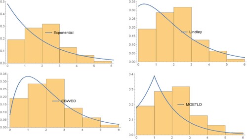
Table 4. Estimation and information criterions for aircraft data.

Distribution	Parameter	MLE	AIC	BIC	CAIC	HQIC	−2MLL
Exponential	Λ	0.4795	220.597	226.884	223.74	221.44	109.299
Lindley	$\theta$	0.7531	211.156	217.442	214.299	211.99	104.578
MOETLD	$\phi$	1.2908	249.508	262.081	255.795	251.194	122.754
EB-WED	Λ	0.9030	260.23	212.516	209.373	207.073	102.115

Table 5. Distribution fitting tests for the aircraft data.

Model	C-M(W)	A-D	Chi-square	P-value
Exponential	0.7815	3.8916	31.8095	0.0004
Lindley	0.2865	1.7215	19.2381	0.0373
MOETLD	3.24644	16.2276	43.682	0.0000
EB-WED	0.1821	1.0136	9.8095	0.4573

Based on the values of the AIC, BIC, CAIC and HQIC tests the Entropy-Based Exponential Weighted Distribution provides the best fit for the data. Based on the chi-square test for distributions, the proposed weighted distribution shows a significant result to fit the Aircraft data with p-values of 0.45 for EB-WED. This means the proposed distributions are more suitable than the other distributions in fitting the Aircraft data.

13. Concluding remarks

In this article, we proposed a new exponential type of probability density function called the Entropy-Based Weighted Exponential Distribution. Several of its statistical properties, such as the moments’ measures, variability and distribution measures, reliability, hazard, reversed hazard and odds functions, are provided and studied. Moreover, Fisher information and the Maximum-likelihood estimators of the model parameters are obtained. Finally, a real dataset on the Aircraft’s windshield component is analysed and the results are compared to several life-time models. The results showed that the proposed entropy-based exponential model is more flexible and has a better fit for the suggested data.

In this article, we used the Shannon entropy to formulate the weighted distribution. The proposed distribution could be considered a new value distribution that could be used for fitting real-life data. Note that dealing with entropy measures in formulating a new lifetime distribution is not an easy task; however, the window of further research is still open, for example, one can use other entropy measures such as Renyi or Tsallis in formulating the weighted distribution; and the results could be used to compare the new suggested models with the proposed model in this article in terms of model flexibility and bathtub and other reliability measures.

Disclosure statement

No potential conflict of interest was reported by the author(s).

References

- Fisher RA. The effects of methods of ascertainment upon the estimation of frequencies. Ann Eugen. 1934;6(1):13–25.
- Rao CR. On discrete distributions arising out of methods of ascertainment. In: Patil GP, editor. Classical and contagious discrete distribution. Calcutta: Pergamon Press and Statistical Publishing Society; 1965, 27(2); p. 311–324.
- Cox DR. Some sampling problems in technology. In: Johnson NL, Smith H, editor. New developments in survey sampling. New York: John Wiley and Sons; 1968. p. 506–527.
- Al-Nasser AD, Al-Omari A, Ciavolino E. A size-biased Ishita distribution and application to real data. Qual Quant. 2019;53(1):493–512.
- Shannon CE. A mathematical theory of communication. Reprinted with Corrections from the Bell Syst Tech J. 1948;27(3):379–423.
- Rezzoky A, Nadhel Z. Mathematical study of weighted generalized exponential distribution. Journal of the College of Basic Education. 2015;21(89):165–172.
- Mir K, Ahmed A, Reshi J. Structural properties of length biased Beta distribution of first kind. American Journal of Engineering Research. 2013;2:01–06.
- Mudasir S, Ahmad S. Structural properties of length-biased Nakagami distribution. International Journal of Modern Mathematical Sciences. 2015;13(3):217–227.
- Shi X, Broderick O, Pararai M. Theoretical properties of weighted generalized Rayleigh and related distributions. Theoretical Mathematics and Applications. 2012;2:45–62.
- Ye Y, Oluyede B, Pararai M. Weighted generalized Beta distribution of the second kind and related distributions. Journal of Statistical and Econometric Methods. 2012;1:13–31.
- Das K, Roy T. Applicability of length biased generalized Rayleigh distribution. Advances in Applied Science Research. 2011;2:320–327.
- Jabeen S, Jan T. Information measures of size biased generalized Gamma distribution. International Journal of Scientific Engineering and Applied Science. 2015;1:2395–3470.
- Aleem M, Sufyan M, Khan N. A Class of Modified weighted Weibull distribution and its properties. American Review of Mathematics and Statistics. 2013;1:29–37.
- Castillo J, Casany M. Weighted Poisson distribution for over dispersion and under dispersion solutions. Annals of Institute of Statistical Mathematics. 1998;50:567–585.
- Larose D, Dey D. Weighted distributions viewed in the context of model selection: A bayesian perspective. Test. 1996;5(1):227–246.
- Mahfoud M, Patil G. On weighted distributions. In: Kallianpur G. et al. editors. Statistics and probability essays in honor of C. R. Rao. Amsterdam: North-Holland Publishing Company. 1982; p. 479–492.
- Al-Kadim A, Hussein A. New proposed length biased weighted exponential and rayleigh distributions with application. Mathematical Theory and Modeling. 2014;4(7):137–52.
- Al-Kadim K, Hantoosh A. Double weighted distribution and double weighted exponential distribution. Mathematical Theory and Modeling. 2013;3(5):124–34.
- Bashir S, Rasul M. Some properties of the weighted Lindley distribution. International Journal of Economics and Business Review. 2015;3:11–17.
- Modi K. Length-biased weighted Maxwell distribution. Pakistan Journal of Statistics and Operation Research. 2015;11:465–472.
- Kharazmi O, Mahdavi A, Fathizadeh M. Generalized weighted exponential distribution. Communications in Statistics – Simulation and Computation. 2014;44(6):1557–1569.
- Renyi A. On measures of entropy and information. In: Jerzy Neyman editor. Proceedings of the 4th Berkeley symposium on mathematical statistic and probability. Vol. I. Contributions to Probability and Theory. Berkeley: University of California Press; 1961. p. 547–561.
- George D, George S. Marshall–Olkin Esscher transformed Laplace distribution and processes. Braz J Prob Stat. 2013;27(2):162–184.
- Lindley DV. Fiducial distributions and Bayes’ Theorem. J R Stat Soc. 1958;20:102–107.
- Maydeu A, Garci A, Forero C. Goodness-of-Fit testing. International Encyclopedia of Education. 2010;7:190–196.
- Schwarz G. Estimating the dimension of a model. Ann Stat. 1978;6(2):461–464.
- Akaike H. A New look at the statistical model identification. IEEE Trans Autom Control. 1974;19(6):716–723.
- Bozdogan H. Model selection and Akaike’s information criterion (AIC): the general theory and its analytical extensions. Psychometrika. 1987;52(3):345–370.
- Hannan EJ, Quinn BG. The determination of the order of an autoregression. J R Stat Soc B Methodol. 1979;41(2):190–195.
- Heggland K, Lindqvist BH. A nonparametric monotone maximum likelihood estimator of time trend for repairable systems data. Reliab Eng Syst Saf. 2007;92:575–584.
- Stephens MA. EDF statistics for goodness of Fit and some comparisons. J Am Stat Assoc. 1974;69:730–737.
- Cramér H. On the composition of elementary errors. Scand Actuar J. 1928;1928(1):13–74.
- Laha C, Laha RG. Handbook of methods of applied statistics. New York: John Wiley and Sons; 1967. 1; p. 392–394.
- Murthy DNP, Min X, Jiang R. Weibull models. New York: John Wiley and Sons; 2004. 1047(22).
- Blischke WR, Prabhakar Murthy DN. Reliability: modeling, prediction, and optimization. New York: John Wiley and Sons; 2011.