Development of species recognition models using Google teachable machine on shorebirds and waterbirds

Abstract

Species identification is an essential ability in every conservation initiative. An efficient and robust computer vision method was attested with an available online tool with Google's Teachable Machine. This pilot study on developing a species recognition app was to create and evaluate the usability and accuracy of using Teachable Machine for species identification at Teluk Air Tawar, Kuala Muda (TAT-KM), Malaysia. The accuracy of the created models was evaluated and compared with training images based on the web-mining (Google Images Repository) compared to actual photos taken at the same site. Model A (Google Image) had an average accuracy of 55.30%, while Model B (actual photos) was 99.42%. Regarding success rate at accuracy over 77%, 27 out of 49 test images (55.10%) were reported in Model A, while Model B had a 100% success rate. This approach can replace traditional methods of bird species recognition to handle large amounts of data.

KEYWORDS:

• Machine learning
• Google teachable machine
• species classification
• shorebirds
• important bird area

1. Introduction

Species recognition is the most crucial step in any zoological research and conservation. Traditionally, scientists rely on their experience and handbooks to identify the animal species in the field, which is tedious and time-consuming for data collection and analyses. However, as computers become an inextricable part of our daily lives, more and more wildlife researchers benefit from the convenience and effectiveness of machine learning and computer vision in recent decades.

Machine learning is increasingly popular over the recent decades with the booming of the digital revolution that powers everyday tools from speech recognition in Siri to autonomous vehicles in Tesla. Machine learning is a subset of artificial intelligence that improves computational algorithms automatically through experience [1]. It is built based on training data as samples to make predictive analysis and generate outcomes without being programmed directly [2]. Machine learning typically creates a model based on the training data that can be attested by a separate test dataset.

Machine Learning is a field of artificial intelligence that helps computers learn from data to perform tasks independently. The first and most fundamental task of machine learning is identifying data patterns. This machine learning algorithm can then make decisions about new data based on past data. In simple words, machine learning is a technology that allows machines to learn from data without being explicitly programmed. It can be applied to various domains, including computer vision, speech recognition, and natural language processing [3–15]. Popular machine learning algorithms include neural networks, decision trees, and support vector machines. Machine Learning is one of the most important and widely used technologies in biological research. It offers several advantages, such as the ability to collect data and analyse it without having to programme it, and the ability to identify trends and patterns to extract useful insights that can be used to optimize processes. It also can increase organizational efficiency by reducing the need for human intervention. However, there are also some disadvantages, such as the risk of accidentally introducing bias into the machine's decision-making process.

In ecology, there are numerous research areas where machine learning can be a useful tool. For example, it can be used to identify patterns in ecological data that are often difficult or impossible for humans to spot on their own. Species classification has been made simple and more adaptable to scientists and the public using image classifications. Certain apps such as Inaturalist, PlantSnap, and SnapCode use machine learning to identify species based on images. In plant breeding, machine learning can be used to select plants based on their predicted performance, thus reducing the amount of time it takes to breed a new variety or create a new variety of an existing crop. Machine learning is also used to count trees, which can be useful in ecological survey analysis [16]. It can also be used to determine the spread of pests or diseases, such as by predicting which species are most vulnerable to a certain disease, which was a crucial analysis during the pandemic [17]. Researchers at Queensland University of Technology (QUT) developed a new machine learning mathematical system that helps identify and detect biodiversity changes, including land clearing, when satellite imagery is obstructed by clouds [18]. One of the key advantages of using Machine learning in ecology is the ability to discern complex data analysis involving data sharing, meta-data analysis and citizen science [19]. One key area that could benefit from citizen science input is the study of migration. Migratory animals such as birds migrate across continents, requiring the combined effort of observers in multiple countries. Data sites such as Ebird, presents a good platform for data sharing.

Shorebirds and waterbirds are prominent birds commonly found across beaches, mudflats, mangroves, and wetlands in the intertidal zone. Migratory shorebirds live on the bay, wetland, ocean, and lake coasts, where they need to relax and feed for their yearly migration during the non-breeding season [20]. Malaysia serves as a biodiversity hotspot with a total of 718 species of birds, 239 of them being migratory. Most migratory birds in Malaysia are on the migration route between their breeding and wintering areas called the East Asian-Australasian Flyway (EAAF), stretching from north to the arctic to the south of New Zealand.

Google's Teachable Machine (https://teachablemachine.withgoogle.com) is a web-based tool for developing machine learning models that are quick, simple, and open to anybody. This study uses the Teachable Machine as the main tool for species recognition and classification. Then, the accuracy of the model was evaluated to ensure the algorithm's stability. Developing a machine learning model for species recognition requires special expertise from computer sciences and programming. In addition, more applications and software integrate machine learning and computer vision in parts of the algorithm. Developing a robust machine learning-based approach locally can expedite the current shorebirds conservation projects and studies due to its simplicity and correctness. Machine Learning is utilized for species recognition to evaluate the functionality of using Google's Teachable Machine in this study.

This study will introduce a simple bird species recognition method using Google's Teachable Machine. The research question is to evaluate whether different sets of training database can affect the accuracy of the Teachable Machine Tensorflow algorithm. One dataset would be gathered from online repository while the other would use images directly from the sampling areas. Teachable Machine is a web-based platform for creating personalized classification model machines without professional technological knowledge. Internet users have created over 125,000 machine learning models with Teachable Machine. It allows all ranges of people such as teachers, students, and others to create their classification model based on built-in machine learning technology powered by TensorFlow.

The latest version of Teachable Machine accepts three main kinds of inputs from users: image, audio, and pose via webcam or upload. Teachable Machine can recognize countless objects from daily life even with limited input from users. Users can create models based on random objects to create classes as long as they provide data input and classifications. This is because the Teachable Machine was built in such a way that it does not require much data or high computing power for creating accurate models [21].

Teachable Machine has a simple interface that serves as a quick, easy tool to classify input using any training images, audio, or videos. Toivonen et al. [22] have shown this tool's feasibility and efficiency by designing their Machine learning-powered applications with students from kindergarten to 12th grade in the US. Teachable Machine has also been demonstrated to aid blind users using teachable object recognizers in real-world scenarios [23]. With all these examples, Carney et al. [21] highlighted a few main contributions of Teachable Machines, which are (1) user-friendly interface, (2) no coding or machine learning experience needed, (3) providing future interactive machine learning tools and lastly (4) simplified machine learning concept for ease of teaching or learning. In other words, it can allow people with different expertise to utilize machine learning without related knowledge and technical difficulties.

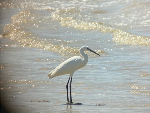
It is important to iterate that our study will not focus on the complex and detailed machine learning analysis. For comparison, Xu and Zhu [24] conducted a thorough and extensive study of seabirds identification using a modified Grabcut technique achieving an impressive 88.1% accuracy. Atanbori et al. [25] implemented a new technique integrating appearance and motion to increase the accuracy of the available deep learning models. Compared to these two studies, our study only uses a simple click and drag interface, which required almost no coding knowledge. This pilot study aims to use Teachable Machine as a primary tool to identify different shorebird species at TAT-KM. Computer vision can be used for image-based species identification if given enough data to the neural network. The type of machine learning used in this research is supervised learning, where images of shorebirds were collected and used to associate the input with the desired output. In this study, the desired output is building a fast, accurate model that can precisely categorize the shorebird species into different classes. A total of seven classes of most common shorebird species at Teluk Air Tawar Kuala Muda (TAT-KM), Malaysia, were selected and tested with Google's Teachable Machine, which was: Asian dowitcher (Limnodromus semipalmatus), brown-headed gull (Larus brunnicephalus), common redshank (Tringa totanus), great egret (Ardea alba), little egret (Egretta garzetta), pond heron (Ardeola sp.), and whiskered tern (Chlidonias hybrida).

The accuracy of the models created with Teachable Machine will be evaluated and compared with training images based on web-mining (Google Images Repository). To the best of our knowledge, this is an original study that uses a simple Guided User Interface (GUI) such as the Google Teachable Machine to compare the efficacy of using datasets gathered from two technique. This technique, if successful, can replace traditional methods of bird species recognition to handle a large amount of data. Researchers can also apply such an approach to other types of morphologically similar species and develop a feasible yet accurate species recognition app themselves.

This manuscript is divided into Introduction, Methodology, Results and Discussion. An extended literature review concerning machine learning will be included in the introduction. A concise systemic method review will be included in the early part of the methodology.

2. Methodology

2.1. Study site

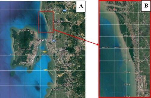
The project took place at Teluk Air Tawar-Kuala Muda (TAT-KM) Coastin Kedah, Malaysia, as shown in Figure 1. Shorebird survey was carried out at intertidal mudflat of Teluk Air Tawar, Kuala Muda (TAT-KM) coast extending from Taman Teluk Molek (approx. 5°28′41.9′′N 100°22′44.4′′E) in the south to the south shore of Sungai Muda (approx. 5°34′35.8′′N 100°20′22.6′′E). TAT-KM Coast is situated between the state of Kedah (north) and the border of Penang (south). The selected study area comprises nearly 200 hectares of mangrove forest and 200 hectares of marshes. The IBA is roughly 8 km long and 1 km broad on average. The selection of the site is supported by the status of TAT-KM as an IBA (Important Bird Area) with a high conservation value [26]. Shorebird surveys were undertaken in March 2021 at TAT-KM. Morphological characteristics and features of 15 selected bird species at the TAT-KM coast were studied beforehand. TAT-KM was surveyed using birding scopes accompanied by bird expert Dr Nur Munira Azman (https://www.facebook.com/shorebirdspeninsularmalaysia/) to verify the data collection. Specifically, three locations were in TAT-KM were chosen, which were Warung Kulat Kuala Sungai Abdul Bagan Belat (5°29′48′′N, 100°22′40′′E), Mee Udang Seri Pantai (5°32′26′′N, 100°2′11′′E), and Bakau Tua (5°34′4′′N, 100°20′48′′E).

Figure 1. (A) Penang map with a red square indicating the location of TAT-KM. (B) Site map of TAT-KM. (Google, n.d.).

2.2. Systematic review of current available techniques for Machine Learning

Machine Learning is the process of making a computer system learn how to do tasks on its own, without being explicitly programmed. Multiple platforms are available to perform Machine Learning, the most common ones being; Mathematica, Python, R, Mathlab, Roboflow and Google Teachable Machine. Each one of these platforms has different strengths and weaknesses, which will be discussed in more detail below.

Multiple platforms are available to perform Machine Learning, the most common ones being; Mathematica, Python, R, Mathlab, Roboflow and Google Teachable Machine. Each one of these platforms has different strengths and weaknesses, which will be discussed in more detail next.

Mathematica (Mathematica) is a programming language developed by Wolfram Alpha Inc., which is used for modelling and data analysis. It is a great tool for academics and researchers, but it is very time consuming to learn. Furthermore, there is no free version available for personal use. Fadzly et al [27] used Mathematica platform to evaluate whether AI can be fooled by nature's mimicry. Their results showed that the system could differentiate between bees and orchids with a high degree of accuracy despite only seeing parts of it. One of the most interesting features is the natural language syntax, the ability to offload the calculations on Wolfram Server and the software's ability to determine which algorithm best suits the input data.

Python is another commonly used platform for performing Machine Learning, an open-source environment for analysing, processing and visualizing data. It is currently the most famous and top-used language for programming. It's open-source and free. Similar to Mathematica, Python can also be used to develop mathematical models to solve real-world problems. However, Python requires much programming knowledge to use effectively, and its learning curve is very steep. One of the main drawbacks of using Python is that it lacks a user-friendly interface, making it less user-friendly than some other options available. Cholet [28] outlined a detailed analysis and framework of Object Detection, Model Creation and several Deep Learning models such as Keras, TensorFlow, Yolo and several others. The huge advantage of Python is it is free, there are a huge number of libraries available.

R is also a free open-source statistics software that is extremely useful for performing data mining and statistical analysis. The large number of functions it supports makes it ideal for research purposes. However, it is not particularly user-friendly and can be quite time-consuming to learn. Therefore, it is not ideal for non-specialist users. Although there are GUI built for R such as R Commander and R Studio, these may not be an ideal solution if the data being analysed is in a format that is difficult to manipulate. R Studio, however, provides Machine Learning tools allowing for easy customization of models and tasks and exporting data for analysis in other tools (https://tensorflow.rstudio.com/tutorials/keras/classification).

Mathlab is a platform for performing mathematical computations, similar to Mathematica, Phyton, and R. It can be used for all sorts of mathematical operations, including calculus, linear algebra, signal processing and statistics. However, like both Phyton and Mathematica, Mathlab is not particularly user-friendly and has a steep learning curve. Singh et al, (2017) used K- means clustering algorithm to identify different images of plant disease focusing on the Anthracnose disease via Matlab.

Roboflow is a free web-based software platform that can be used to carry out numerical analysis, simulation and machine learning applications. It can also create Internet of Things (IoT) devices and remotely control robots. Roboflow makes creating innovative interactive applications and prototypes easy without writing any code. The platform offers a wide range of prebuilt functions that can be used to design applications quickly. Even though there are basic free version for Roboflow, there are limitations for the algorithm and the dataset. The free version requires the dataset to be publicly available. Similar with Google Teachable Machine, the calculations is done in the cloud using Roboflow Virtual Machine.

Google Teachable Machine is a machine learning platform that allows users to build their own models without coding. Users can then deploy these models to Google Cloud to automatically process and analyse data without human intervention. It can be accessed through a web browser or via a mobile app and can be used to build models for a wide range of tasks including computer vision, speech recognition and more. The main advantage would be its accessibility (free) and simple Graphical User Interface (GUI), which greatly simplifies the training process and makes it accessible to everyone from beginners to professionals. The weakness would be that it is not as powerful and advanced as other ML platforms.

2.3. Field sampling

The main purpose of the field sampling was to take photos of the selected shorebird species at TAT-KM to be used as a reservoir in model training. A total of 550 images of related shorebird species were taken manually with iPhone 11 attached on a spotting scope. The process started by setting up required equipment such as tripods and two spotting scopes at the TAT-KT study sites, which were at least 100 m away from the shorebirds. Shorebird species recognition was verified by shorebird experts Dr Nur Munira Azman, Mr Nasir Azizan (from Shorebirds Peninsular Malaysia Project) and Boarman [29]. The photos of shorebirds were taken at the designated areas on the 9th, 14th, 17th, and 21st in March 2021, which were still in the migration season of shorebirds. During the last two attempts of field sampling, photos were taken on a boat that cruised along the coastline of the study sites. This method could ensure a better view of shorebirds as there were fewer obstacles like trees and rocks as compared to the direct observation from the mudflat. All photos of shorebirds were taken during the daytime, varying from 9 am to 3 pm, to optimize the quality and brilliance of the images. Of all the field visits, the height of the tides was moderate. Direct observation was applied by using binoculars (8 × 42 magnification) and spotting scopes.

2.4. Data processing

2.4.1. Creating supervised learning models

The first objective aims to create supervised learning models for selected shorebird species using Google's Teachable Machine. Two models were built, Model A using images from web-mining (Google Image Repository), and Model B, which was composed of photos of seven (7) selected individual bird species from TAT-KM.

2.4.2. Creating Model A and Model B

Usability and accuracy of Teachable Machine for bird species recognition were first tested using images from web-mining (Google Image Repository). A total of 550 photos of seven selected bird species, namely whiskered tern (Chlidonias hybrida), pond heron (Ardeola spp.), little egret (Egretta garzetta), great egret (Ardea alba), common redshank (Tringa totanus), brown-headed gull (Chroicocephalus brunnicephalus), and Asian dowitcher (Limnodromus semipalmatus) were collected from Google Image Repository. The images for each bird species were downloaded from Google Image Repository using the Download All Images Firefox extension to facilitate the process. All images were filtered manually to ensure that they fulfilled the criteria following: (1) Only photos with a single individual bird were selected, (2) photos with the complex background were discarded, (3) photos must be taken at daytime, and (4) different angles of individual birds were chosen. These criteria can ensure the quality of photos and improve the accuracy of the trained model in the Teachable Machine. The images taken from Google Image Repository were labelled and put into the folder named Database A. 75% of these images were used to build a supervised model using Google's Teachable Machine, while the model accuracy was tested using 25% of the remaining images. 75% of the images were assorted, which were composed of 198 images. These photos were uploaded into Teachable Machine to create and train bird species recognition algorithm, Model A. Then, the remaining 25% of images were used to create a database consisting of 49 test images. These test images contained a mixture of seven (7) selected bird species which were images that were not used in model training; hence no repetitive images were used. The whole procedure was repeated with Model B, which was solely composed of photos taken manually at TAT-KM.

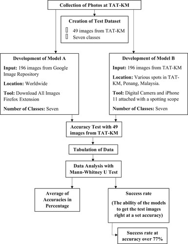
During data collection, photos of the same seven (7) selected individual bird species from TAT-KM were taken using a high-resolution digital camera (Sony RX10 M3) and iPhone 11 attached to a spotting scope. All photos must fulfil the criteria mentioned for Database A. When photo samples were taken, complex backgrounds such as trees, mangroves and residential houses were avoided to increase the clarity of the photos. Different angles of individual birds were taken to improve the accuracy of the trained model in Teachable Machine. 30–50 photos of each bird species were taken. A total of 550 photos were taken and stored in Database B, which consists of actual bird photos taken at TAT-KM. These photos were later filtered manually as some bird photos were not qualified. In the final selection, there were a total of 247 actual bird photos, where 75% of them (198) were used to train Model B. This Database was uploaded into Teachable Machine used to train a new bird species recognition algorithm named Model B. A database consisting of 49 (25%) actual unused photos were used as test images to evaluate the usability and accuracy of the model. A flow chart that summarizes the procedures is shown in Figure 2.

Figure 2. Flow chart of the methodology.

2.4.3. Using Google's Teachable Machine

Google Teachable Machine website was accessed using the researcher's personal Google Account. Seven main classes, which are Whiskered Tern, Pond Heron, Little Egret, Great Egret, Common Redshank, Brown-headed Gull, and Asian Dowitcher, were created after the “image project” category was chosen on the main page of the website. All images collected in Database A and Database B were uploaded in a specific folder in Google Drive. Next, each class in Google Teachable Machines was trained with class images. After that, upon finishing uploading all class images for each class, the “training” button was selected, and the inputs were processed and analyzed by the Machine. Forty-nine test images from seven (7) classes were also collated. It is important to note that these test images were separated from the class images and not subjected to the learning algorithm. Once the processing was completed, the projects were named Model A and Model B, respectively and saved to Google Drive for later use. The TensorFlow models can be viewed from these links.

Table

Model A	https://teachablemachine.withgoogle.com/
	models/KtkMEubHi/
Model B	https://teachablemachine.withgoogle.com/
	models/DRB2UW9Ta/

The models are exported as Tensorflow.js, which is a browser-based project. This simple setup ensures the models can be run by any smart mobile phone with an internet connection. There is also an option to export the models to Tensorflow for advanced manipulation of Python language. Finally, the Tensorflow lite export option is also available to export the models to be run on Android-based phones. The app could be run without an internet connection.

2.4.4. Comparing Model A and Model B

Google Teachable Machine already has a built-in accuracy measurement analysis. The details can be accessed by selecting the “Advance” button and “Under the hood” selection after the model training. We will also display the confusion matrix and the accuracy graph from GTM. The second objective aims to evaluate and compare the models built using Google's Teachable Machine as a tool for bird species identification at TAT-KM. After Model A and Model B were built, both models were tested using 49 test images from actual bird photos taken at TAT-KM to mimic the actual situation whereby researchers use the models to identify bird species. Each class comprises a different number of test images due to the limitations of field sampling. In both models, the accuracy of the model in the percentage of each image was recorded in a table. The average of the accuracy in percentage for each class was calculated and recorded in the table.

Besides the accuracy in percentage, the success rate of each image was recorded. For this study, the success rate was defined as the ability of the models to get the test images right at accuracy in percentages over 77%. This number was chosen as the baseline according to the species accuracy of the iNaturalist application [30]. Hence, accuracy over 77% can be considered as highly accurate as compared to the iNaturalist application, which is an increasingly popular species recognition application worldwide [31]. The number of test images that had accuracy over 77% for each class was counted and recorded in a table. No set accuracy percentage can be considered successful or not. According to Bernard [32], the acceptable accuracy percentages vary based on the application and usage of the model; for example, a 95% accuracy might not be enough for an algorithm to detect possible tumours (from pictures), whereas an 80% accuracy is enough to just differentiate between a cat and a dog.

2.5. Data analysis

After evaluating the accuracies of both Model A and Model B, a spreadsheet composing raw data of accuracies of each test image, average, and the success rate was built. Both models were compared statistically in two ways, (1) average of accuracy and (2) success rate of accuracy at 77%. Since the datasets were non-parametric, Mann–Whitney U Test was used to evaluate the significant difference of both models at a 0.05 significance level for the two-tailed hypothesis. For the second dataset that examined the success rate at 77%, a one-tailed hypothesis was used instead since the test aimed to determine if Model B has higher accuracy than Model A.

3. Results

3.1. Built-in GTM accuracy results

Figures 3 and 4 (Model A and Model B, respectively) shows the confusion matrix results, accuracy and epoch loss from Google Teachable Machine internal analysis. There are a range of performance metrics to evaluate our model, we choose the most basic and already included in the Google Teachable Machine. Confusion matrix shows the actual number of predictions made by the algorithm in comparison with the actual true data in the test dataset. The X axis refers to the predicted value, while the Y axis refers to the actual value. The values would show, how many data were wrongly classified. Accuracy shows how accurate the prediction models are. Epochs are the number of times the model are tested. A good accuracy is indicated by the intercept line between actual accuracy and the test accuracy. However, the number of accuracy is dependent on the type of application. 8.0 might be accurate for a species identification whereas it would not be considered accurate for detecting cancer cells. Loss per epoch indicates the number of errors for each epoch, and in general, the lower the value, the better the model would perform.

Figure 3. (a) The confusion matrix, (b) Accuracy per epoch, (c) Loss per epoch for Model A.

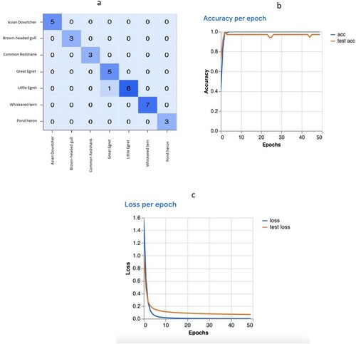
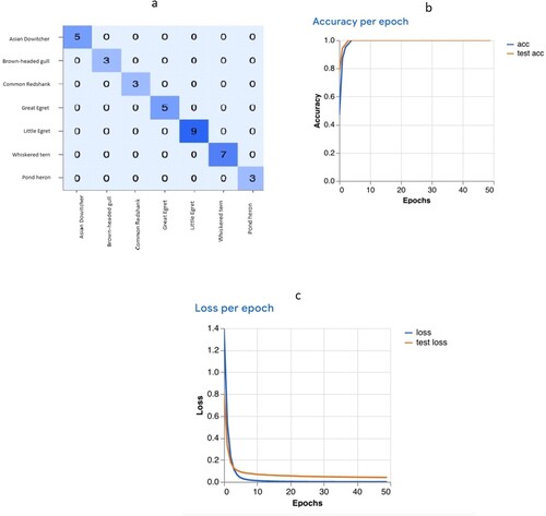
Figure 4. (a) The confusion matrix, (b) Accuracy per epoch, (c) Loss per epoch for Model B.

3.2. Supervised learning models

Two supervised learning models were successfully built using Google's Teachable Machine. Supervised learning models are highly dependent on the number of samples, which in this case, are the training images. Table 1 summarizes the number of training images and test images used in creating both models. The total number of training images was 196 (75%), whereas 49 images (25%) were used as test images. There was a total of 245 images for each model in this study. It is noted that the number of images used in each model was the same.

Table 1. Number of training and test images used in Model A and Model B.

No.	Family	Scientific name	Name of classes	No. of training images	No. of test images
1	Scolopacidae	Limnodromus semipalmatus	Asian Dowitcher	29	7
2	Laridae	Larus brunnicephalus	Brown-headed gull	14	4
3	Scolopacidae	Tringa totanus	Common Redshank	15	4
4	Ardeidae	Ardea alba	Great Egret	29	7
5	Ardeidae	Egretta garzetta	Little Egret	54	13
6	Ardeidae	Ardeola sp.	Pond Heron	14	4
7	Laridae	Chlidonias hybrida	Whiskered Tern	41	10
			Sum	196	49

3.2.1. Accuracies of Model A and Model B

To compare the accuracies between both models, two parameters were used to evaluate the accuracies in terms of the average accuracies and success rate at accuracy over 77%. Figure 5 shows the average accuracy of Model A and Model B.

Figure 5. The average accuracy of Model A and Model B.

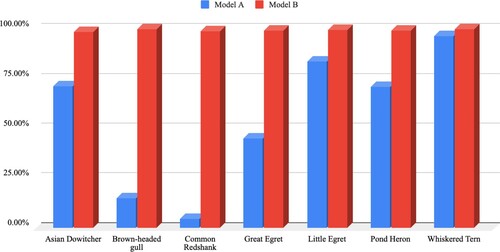
The average accuracy of Model B was also relatively constant, with an average of 99.42% if combined with all classes, whereas Model A has only 55.30%. The mean accuracy of Model B was higher than the mean accuracy of Model A. The mean accuracy of Model B of all classes was 79.78% higher than of Model A on average, with the most significant increase in the class Common Redshank from 4.50% to 99.00%.

A Mann–Whitney U Test was conducted to test the significant difference in the average accuracy of Model A and Model B. The Mann–Whitney U Test shows that There was a significant difference in average accuracy between Model A and Model B, with z = −3.06661, p < 0.05, p = 0.00214.

3.2.2. Success rate of Model A and Model B

For this study, the success rate is defined as the ability of the models to get the test images right at accuracy in percentages over 77%. In particular, the success rate can be calculated as the number of successful test images divided by the total number of test images.

3.2.3. Success rate at accuracy over 77%

Figure 6 shows the number of test images that had a mean accuracy of over 77% in Model A and Model B, respectively. Model B had a 100% in success rate as compared to 55.10% in Model A. In other words, all test images used in Model B had accuracy over 77%, while only 27 test images had accuracy over 77% out of 49 test images in total.

Figure 6. Number of test images with mean accuracy over 77% for each class.

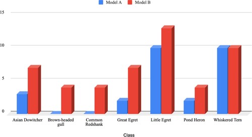
Similarly, Model B performed better and had an equal or higher number of test images with over 77% average accuracy. There was a significant difference in the dataset of both models (Mann–Whitney U test: z = −1.72497, p < 0.05, p = 0.04272). It is worth noting that the performance of both models in the class Whiskered Tern was equal, with 10 test images respectively that had over 77% mean accuracy. The success rate of the class Brown-headed Gull and Common Redshank in Model A were the least satisfactory, with none of the test images scoring over 77%.

4. Discussion

4.1. Morphology of the selected bird species

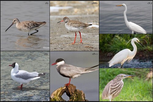
As the models recognize the pattern in the samples, it is important to understand the morphology of the selected bird species, which are included in the seven classes in this study. All image classes were from the order Charadriiformes or Pelecaniformes, which are very specific considering that there are 41 extant orders of birds worldwide [33]. Asian dowitcher, brown-headed gull, common redshank and whiskered tern are from the Order Charadriiformes, while great egret, little egret and pond heron are from the Order Pelecaniformes. Figure 7 demonstrated the examples of training samples of selected bird species used in Model A, which were images from Google Image Repository. Pelecaniformes are typically medium-sized to very large birds with expandable pouches under the bill and webbed feet according to the traditional grouping method [34]. Charadriiformes have a much wider range of morphological features comprising approximately 343 species, as compared to 67 species in Pelecaniformes [35]. The physical parameters of body length, body form, limb length, and bill shape are all highly diverse, making generalizations of morphological patterns of Charadriiformes impossible.

Figure 7. Examples of training samples used in Model A. (I) Asian Dowitcher. (II) Brown-headed Gull. (III) Common Redshank. (IV) Whiskered Tern. (V) Great Egret. (VI) Little Egret. (VII) Pond Heron.

4.2. Accuracy of Model A and Model B

The internal accuracy of Google Teachable Machine shows that while both Model A and Model B scored more than 0.8, Model B does show a much better performance. There were still misclassifications in the confusion matrix for Model A. Accuracy per epoch also shows that the test line did not intercept with the accuracy line, and there was a slight dip during the 20–30 and 40–50 epochs. Epochs refer to the number of passes of the entire training dataset the algorithm has completed. In comparison, there was a perfect intercept for Model B, indicating much better performance. Loss per epoch refers to the loss or the summation of errors value over training per epoch. There was not much of a difference between both models for the loss per epoch.

The objective of this study was to evaluate and compare Model A and Model B. The accuracies of Model A and Model B were statistically compared in two methods: (1) average accuracies and (2) success rate of accuracy at 77%. Of the two methods, one of them has shown that there is a significant difference between the accuracies of Model A and Model B.

Model B performs exceptionally with an average of 99.42% accuracy in terms of average accuracy. All classes in Model B had 98.71% to 100% accuracy in correctly identifying and classifying the selected bird species. This result further ensures the robustness of Model B, which can be used in the field to identify bird species. On the contrary, Model A had 57.63% accuracy only on average, varying from 4.50% to 96.50%. Notably, the classification of the class Brown-headed gull and Common Redshank performed very poorly at 15.00% and 4.50%, respectively. As mentioned, Model A used the images browsed from the Google Image Repository as input (training images), while Model B was composed of the actual images taken in TAT-KM during the sampling period.

The outstanding accuracy in Model B can be explained by (1) temporal variation, (2) greater background consistency in contrast to the targeted bird species and lastly (3) the quality of the images. The training images used in Model B were taken at the various spots in TAT-KM, which are known to have abundant shorebirds as an Important Bird Area [36]. Based on the observation by Razak [37], the average number of shorebird spottings at TAT-KM was between 170 and 386 individuals. To date, there has not been sufficient evidence on the significant morphological differences of the migratory shorebirds due to geographical variation. In other words, the same species of shorebirds in other parts of the world might have similar physical attributes with the migratory shorebirds spotted in TAT-KM. However, there could be other factors that contribute to morphological differences besides geographical variation, that is, temporal variation.

4.2.1. Temporal variation

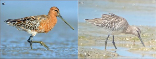
All training images at TAT-KM were taken in March 2021, which was during the middle of the non-breeding season for most migratory shorebirds on the EAAF [38]. This further explained the accuracy difference in the Class Asian dowitcher where all the training samples used in Model B were taken in March, and thus they possessed the morphological features that are seen during non-breeding seasons. Figure 8 shows the images used in Model A and Model B, which demonstrated the different morphologies of Asian dowitchers during non-breeding and breeding seasons. During the breeding season, they have apparent changes in the colour of plumage at the breast, which is evenly chestnut-red. On the other hand, all the reddish plumage is gone in the non-breeding season; the breast and underparts become darkish grey-brown with whitish feather edgings [39]. This could be the reason for the higher numbers of test images with average accuracy over 77% at seven (7) in Model B, as compared to three (3) only in Model A.

Figure 8. The difference in the appearance of the same species Asian dowitcher. (I) An example of a training image used in Model A. The morphological feature of the bird fits the description of the Asian dowitcher in the breeding season. (II) An example of a training image used in Model B. The brownish plumage tells that the bird is not in its breeding season.

4.2.2. Consistency of the background

Besides the temporal variation that might have caused a significant difference in the accuracy of Model A and Model B, the background of the training samples used could affect learning models. Based on the study by Fadzly, Zuharah & Wong [27], machine learning can wrongly target the background as one of the key characteristics for classification. Hence, the inconsistent backgrounds in Model A could possibly confuse the learning model and yield a lower accuracy rate in identifying the selected bird species in TAT-KM. Logically, including different backgrounds and lighting could make a machine model more robust, provided that there is a significant amount of training samples. However, there are only a total of 196 images as training samples in each model due to the time constraint during data collection. Backgrounds serve important roles in object recognition as machine learning models learn the key characteristics of the objects [40]. Machine learning may even use backgrounds in classification and identification [41]. For instance, there were many studies that indicate machine learning models could perform unexpectedly due to dependence on the parameters that humans do not rely on [42–44]. Hence, the properties of the background might have a profound impact on image processing that human eyes do not realize.

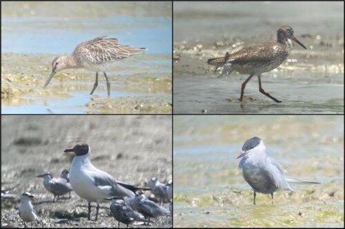
In this study, all classes of training images used in Model A featured various types of backgrounds as the images were taken from the internet randomly. The locations and geographical characteristics of the backgrounds were not being controlled or monitored during the process of data mining of the images from the Google Image Repository. Moreover, it is almost impossible to identify the locations of the birds based on the training images used in Model A. There were no restrictions on the locations of the photos taken as such measures could lead to a bias in random sampling. A few selected examples of training images used in developing Model A are shown in Figure 9, showing different backgrounds as opposed to the actual photos taken at TAT-KM featuring a monotone background. The backgrounds of the training images used in Model B were very consistent in terms of colour, lighting, exposure, saturation and tint, as shown in Figure 10. All the training images in Model B were slightly dull and less saturated than images used in Model A. Even though the images were taken from the various spots in TAT-KM, the tone of the backgrounds did not differ much from each other, with all featuring brown, greyish mudflat as background. With most shorebirds and waders having a similar colour of plumage to their habitat, this is not a coincidence. Most shorebirds have more uniform plumage, like their roosting habitats as camouflage which allows them to be less visible to predators [45]. Although the selected individual birds have lower contrast to their background due to the similar tone, this does not seem to affect the accuracy of the model in general.

Figure 9. Examples of training images of Model A that have complex backgrounds.

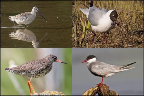
Figure 10. Examples of training images of Model B that have monotone backgrounds.

4.2.3. Quality of the images

The quality of the training images used in both models varied. This is unavoidable due to the fact that the training samples of both models were from different sources. The quality of an image is quantifiable and measurable based on a few parameters, predominantly resolution, which is defined as the pixel count in digital imaging. Normally, the numbers of the pixel count are expressed as the number of pixel columns multiplied by the number of pixel rows (e.g. 4000 × 3000 pixels). Hence, the higher the pixel counts, the greater the details of the image, which would, in turn, produce images with good quality. Other than that, parameters like aperture, ISO, shutter speed, exposure, tint, saturation and others can greatly affect the quality of an image.

Just like digital imaging, machines interpret those images in pixels, and each pixel contains its own value that could be read by the computers, which is normally in the data matrix. These data are the actual input in the machines and are used in the algorithm of the models. Further analyses such as classification, identification and tracking of objects could be conducted. In this study, the main task of the models built is identification since the classification was previously done manually. Since computers’ see’ the image through pixels, the number of pixels becomes an indirect contributing factor to the accuracy of the models built.

The training samples of both models have different sources of input. Model A was composed of images from various websites which were not traceable since the collection of images was done automatically via a browser extension. This caused the image size in pixels to vary widely, ranging from 10 000 pixels (100 × 100) to 24 000 000 or 24 megapixels (6000 × 4000), as shown in Figures 11 and 12. The inconsistency of image quality could greatly affect the outcome of the model built since the model relies on the pixels that contain digital information. When the pixel counts are low, less information can be retained and used during training. This is supported by Lau, Li & Lam [46], in which it was stated that the accuracy of image classification is decreased when the image is compressed. As Model A uses images from the web, most are compressed images. As a result, the accuracy of the model is less promising. On the contrary, the training samples of Model B were sourced from solely two cameras, iPhone 11 and Sony RX10 M3. The iPhone 11 features a 12-megapixel wide-angle lens, while Sony RX10 M3 has a sensor that can produce up to 20.1-megapixel photos. Ideally, the majority of the photos in Model B have 12 megapixels (4032 × 3024) by default, but some images were zoomed and cropped before putting into training, and thus the pixel counts range from 2 megapixels (1607 × 1177) to 12 megapixels (4032 × 3024). The examples are shown in Figures 13 and 14. As a comparison, Model B has a very consistent and reliable quality of images while Model A lacks uniformity in pixel counts, which affects the accuracy of the model.

Figure 11. One of the training images in Model A. This image has 10 000 pixels (100 × 100).

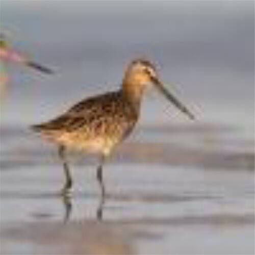
Figure 12. One of the training images in Model A. This image has 24 megapixels (6000 × 4000).

Figure 13. One of the training images in Model B. This image has 2 megapixels (1607 × 1177).

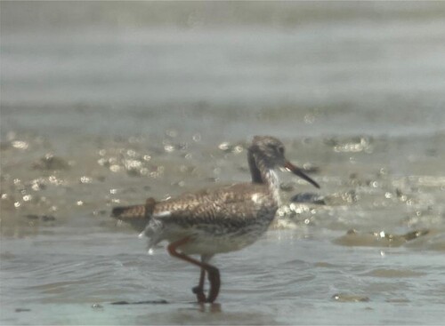
Figure 14. One of the training images in Model B. This image has 12 megapixels (4032 × 3024).

4.3. Machine learning vs humans

An improvement in technology or any innovation in science always aims to make a human's life easier and better. Given the results from this study, it is important to know if the proposed technique expedites the traditional process of bird species recognition. Other than the time required, attributes like energy, feasibility, portability, and flexibility of the methods should be considered in species recognition. Both computers and humans utilize very different approaches to identifying animals. Humans are carbon-based machines; their eyes are the result of the million years of evolution. Their silicon counterparts, computers, are made to imitate the nature of the processing algorithm of humans, which is the neural network. The intrinsic differences in both thought processes of humans and computers result in some pros and cons for both methods.

Machines can only interpret what they have been taught in the original dataset, which means they are more likely to regurgitate the information they have already gathered. As a result, every time a new set of data or images are added as training samples, the accuracy of the models will vary and fluctuate. In this case, Google's Teachable Machine could have limited ability to adjust to different real-world circumstances unless special algorithms, codes or different inputs were fed into the system. Hence, the main disadvantage of using this Machine is that it requires a large number of inputs to produce an accurate result. However, one of the main advantages of using Google Teachable Machine is the time and computing power to train the model. Normally, training on a local computer would require a huge amount of RAM and would be taxing on a discrete central processor. While the task load could be mitigated by using graphic cards (especially the NVIDIA RTX series), there is an additional cost involved. Google Teachable Machine uses virtual Machines, and the models are trained on the cloud. The training is free, fast and efficient, requiring very little resource from the user.

Previous scholars (e.g. [47,48]) emphasize the potential for deep learning to increase the number of samples and therefore help resolve some of the common limitations in power for zoological studies (e.g. [49]). When encountering large amounts of data, humans get exhausted easily if they were to identify the bird species one by one. As the computing technology becomes more advanced, it would take only the time of a blink of an eye to accurately identify, sort and classify any inputs, provided that the model is well trained beforehand. After a specific animal recognition model is trained, it can be used for the long term if the morphology of the animals remains constant. The trained model can even be shared with other scientists easily if they intend to use the model as a quick animal recognition tool.

Though only available on the website, Google's Teachable Machine provides the option that allows users to save and export their models for offline use. Computer-generated codes of the model in JavaScript are also available to download easily after the model is trained, which allows users to investigate, modify, edit and export for other use, such as mobile app development. A designated localized species recognition can be done much more feasibly with just a mobile application. Hence, the use of Google's Teachable Machine is versatile and flexible, with many possibilities provided. Not only more time is saved, but the energy and time can also be shifted into investing in other steps in research.

5. Conclusion

The biggest limitation throughout the study was the nationwide COVID-19 restrictions imposed in Malaysia, which constrained us from going to the field for samplings. As a pilot study using Google's Teachable Machine in shorebirds and waterbirds, this study provided a brief insight on the simple method to identify important bird species without any pre-existing computing knowledge. This research is feasibly replicable. Our original aim was to create a simple species recognition app that could be integrated into citizen science and nature education camp for kids. We aim to test the accuracy of the kids using the app compared to using an identification book. Both activities are usually handled by the Peninsular Shorebirds organizations. Unfortunately, we are still unable to conduct these camps due to COVID restrictions. Furthermore, the number of sampling trips was drastically reduced. Otherwise, it is recommended to increase the sample sizes of all classes of bird species to create more robust models. Besides comparing both models, further analyses can be done on notable images, such as using more advanced machine learning tools like Wolfram Mathematica to pinpoint and highlight the key characteristics of the images that Machine uses to identify the bird species.

Finally, in terms of using Google Teachable Machine, the main advantage (which is easy to use) is also its biggest limitation. The platform offers a basic web app approach (that is automatically created), the results would show the probability percentage of each species compared. If this was used on a phone with a small display, it would cause the display to be constrained and there is no option to just show just the top three results. This however can be rectified with a bit of programming in Python. Another weakness would be that this would be only tailored to the shorebirds, even if you point the camera to another animal (for example a chicken), the algorithm will still try to calculate the nearest classification of it. Another limitation would be that the app would only show the percentage probability, there is no option to include trigger commands, for example if a certain species is detected, we could trigger the command to bring up facts about it on the side panel. This would be possible, but you would need further programming in Python.

However, if the main aim is only to create a simple identification app for a limited number of species, using data directly from the species original habitat, then Google Teachable Machine would be the most suitable option. It is free, easy to access, easy to deploy and it still does offer further improvement or refinement through porting the model into another language (Python, C, C++). It can be used by beginners (even school children) and also offers options to be used by intermediate programmers.

Disclosure statement

No potential conflict of interest was reported by the author(s).

Additional information

Funding

This work was supported by Universiti Sains Malaysia [grant numbers 304/PBIOLOGI/6501144.l145; 1001/PBIOLOGI/8011124].

References

- Mitchell T. Machine learning. New York: McGraw Hill; 1997; ISBN 0-07-042807-7. OCLC 36417892.
- Koza JR, Bennett FH, Andre D, et al. Automated design of both the topology and sizing of analog electrical circuits using genetic programming. In: Artificial intelligence in Design'96. Dordrecht: Springer; 1996. p. 151–170.
- Onan A, Korukoğlu S, Bulut H. Ensemble of keyword extraction methods and classifiers in text classification. Expert Syst Appl. 2016;57:232–247.
- Onan A, Korukoğlu S. A feature selection model based on genetic rank aggregation for text sentiment classification. J Inf Sci. 2017;43(1):25–38.
- Onan A, Korukoğlu S, Bulut H. A hybrid ensemble pruning approach based on consensus clustering and multi-objective evolutionary algorithm for sentiment classification. Inf Process Manag. 2017;53(4):814–833.
- Onan A. An ensemble scheme based on language function analysis and feature engineering for text genre classification. J Inf Sci. 2018;44(1):28–47.
- Onan A. Biomedical text categorization based on ensemble pruning and optimized topic modelling. Comput Math Methods Med. 2018;2018:2497471. doi:10.1155/2018/2497471.
- Onan A.. Consensus clustering-based undersampling approach to imbalanced learning. Scientific Programming. 2019;2019:5901087. doi:10.1155/2019/5901087.
- Onan A. Two-stage topic extraction model for bibliometric data analysis based on word embeddings and clustering. IEEE Access. 2019;7:145614–145633.
- Onan A. Topic-enriched word embeddings for sarcasm identification. In: Silhavy R, editor. Software Engineering Methods in Intelligent Algorithms. CSOC 2019. Advances in Intelligent Systems and Computing Vol. 984. Cham: Springer; 2019. p. 293–304. doi:10.1007/978-3-030-19807-7_29.
- Onan A. Mining opinions from instructor evaluation reviews: a deep learning approach. Comput Appl Eng Educ. 2020;28(1):117–138.
- Onan A. Sentiment analysis on product reviews based on weighted word embeddings and deep neural networks. Concurr Comp Pract Exp. 2021;33(23):e5909.
- Onan A. Sentiment analysis on massive open online course evaluations: a text mining and deep learning approach. Comput Appl Eng Educ. 2021;29(3):572–589.
- Onan A, Toçoğlu MA. A term weighted neural language model and stacked bidirectional LSTM based framework for sarcasm identification. IEEE Access. 2021;9:7701–7722.
- Onan A. Bidirectional convolutional recurrent neural network architecture with group-wise enhancement mechanism for text sentiment classification. J King Saud Uni Comput Inf Sci. 2022;34(5):2098–2117.
- Parisa Z, Nova M. This AI can see the forest and the trees. IEEE Spectr. 2020;57(8):32–37.
- Vaishya R, Javaid M, Khan IH, et al. Artificial intelligence (AI) applications for COVID-19 pandemic. Diabetes Metab Syndr Clin Res Rev. 2020;14(4):337–339.
- Holloway-Brown J, Helmstedt KJ, Mengersen KL. Interpolating missing land cover data using stochastic spatial random forests for improved change detection. Remote Sens Ecol Conserv. 2021;7:649–665.
- Humphries GRW, Huettmann F. Machine learning in wildlife biology: algorithms, data issues and availability, workflows, citizen science, code sharing, metadata and a brief historical perspective. In: Humphries G, Magness D, Huettmann F, editors. Machine learning for ecology and sustainable natural resource management. Cham: Springer; 2018. p. 3–26. doi:10.1007/978-3-319-96978-7_1.
- Spencer J. Migratory shorebird ecology in the Hunter estuary, sourth-eastern Australia; 2010.
- Carney M, Webster B, Alvarado I, et al. Teachable machine: approachable web-based tool for exploring machine learning classification. In: Extended Abstracts of the 2020 CHI Conference on Human Factors in Computing Systems. 2020 Apr. p. 1–8.
- Toivonen T, Jormanainen I, Kahila J, et al. Co-designing machine learning apps in k–12 with primary school children. In: 2020 IEEE 20th International Conference on Advanced Learning Technologies (ICALT). IEEE; 2020 Jul. p. 308–310.
- Kacorri H. Teachable machines for accessibility. ACM SIGACCESS Access Comput. 2017;119:10–18.
- Xu S, Zhu Q. Seabird image identification in natural scenes using Grabcut and combined features. Ecol Inform. 2016;33:24–31.
- Atanbori J, Duan W, Shaw E, et al. Classification of bird species from video using appearance and motion features. Ecol Inform. 2018;48:12–23.
- BirdLife International. Country profile: Malaysia; 2020. [cited 2020 Oct 20]. Available from: http://www.birdlife.org/datazone/country/malaysia.
- Fadzly N, Zuharah WF, Jenn Ney JW. Can plants fool artificial intelligence? Using machine learning to compare between bee orchids and bees. Plant Signal Behav. 2021;16(10):1935605.
- Chollet F. Deep learning with python. New York: Simon and Schuster; 2021.
- Boarman WI. A field guide to the birds of West Malaysia and Singapore. Condor. 2003;105(1):169.
- Wäldchen J, Mäder P. Machine learning for image based species identification. Methods Ecol Evol. 2018;9(11):2216–2225.
- Unger S, Rollins M, Tietz A, et al. Inaturalist as an engaging tool for identifying organisms in outdoor activities. J Biol Educ. 2020;55(5):537–547.
- Bernard E. Introduction to machine learning. Champaign (IL): Wolfram Media Publishing; 2021.
- Sullivan BL, Wood CL, Iliff MJ, et al. Ebird: A citizen-based bird observation network in the biological sciences. Biol Conserv. 2009;142(10):2282–2292.
- Causey D, Padula VM. The pelecaniform birds. Encycl Ocean Sci. 2013;4:2128–2136.
- BioExplorer.net. Order Charadriiformes / Shorebirds. Bio Explorer. [cited 2021 July 12]. Available from: https://www.bioexplorer.net/order-charadriiformes/.
- Yeok FS, Aik YC, Butt C. A pilot rapid assessment of selected ecosystem services provided by the Teluk Air Tawar-Kuala Muda coast IBA in Pulau Pinang; 2016. doi:10.13140/RG.2.2.24060.33927.
- Razak N. Shorebird Abundance and Species Richness in Penang Island; 2020. 615–628. doi:10.15405/epsbs.2020.10.02.56.
- Hansen BD, Fuller RA, Watkins D, et al. Revision of the East Asian-Australasian Flyway population estimates for 37 listed migratory shorebird species. Unpublished report for the Department of the Environment. BirdLife Australia, Melbourne. 2016.
- Marchant J, Hayman P, Prater T. Shorebirds. London: Bloomsbury Publishing; 2010.
- Xiao K, Engstrom L, Ilyas A, et al. Noise or signal: The role of image backgrounds in object recognition; 2020. arXiv preprint arXiv:2006.09994.
- Sagawa S, Koh PW, Hashimoto TB, et al. Distributionally robust neural networks for group shifts: On the importance of regularization for worst-case generalization; 2019. arXiv preprint arXiv:1911.08731.
- Jo J, Bengio Y. Measuring the tendency of CNNs to learn surface statistical regularities. 2017. arXiv preprint arXiv:1711.11561.
- Jacobsen JH, Behrmann J, Zemel R, et al. Excessive invariance causes adversarial vulnerability. 2018. arXiv preprint arXiv:1811.00401.
- Jetley S, Lord NA, Torr PH. With friends like these, who needs adversaries? 2018. arXiv preprint arXiv:1807.04200.
- Ferns PN. Plumage colour and pattern in waders. Bull-Wader Study Group. 2003;100:122–129.
- Lau WL, Li ZL, Lam KK. Effects of JPEG compression on image classification. Int J Remote Sens. 2003;24(7):1535–1544.
- Seeland M, Rzanny M, Alaqraa N, et al. Plant species classification using flower images—a comparative study of local feature representations. PloS One. 2017;12(2):e0170629.
- Tabak MA, Norouzzadeh MS, Wolfson DW, et al. Machine learning to classify animal species in camera trap images: applications in ecology. Methods Ecol Evol. 2019;10(4):585–590.
- Wang D, Forstmeier W, Ihle M, et al. Irreproducible text-book “knowledge”: the effects of color bands on zebra finch fitness. Evolution. 2018;72(4):961–976.