Mathematical modelling of growth of tumour cells with chemotherapeutic cells by using Yang–Abdel–Cattani fractional derivative operator

Abstract

Cancer is a fatal disease for a very long time. It has its own history. Now it has become one of the major reasons for death due to its various types. Researchers, scientists and doctors are trying to find out the success and minimize the death rate in this field. The fact is, cancer treatment is only effective when it has been diagnosed at a very early stage. Therefore, cancer is a kind of provocative topic for analysis. In this paper, we have shown the growth of cancer cells, normal cells along with chemotherapeutic cells. We have shown that the effect of chemotherapeutic drugs is highest at the centre of tumour affected area. We have used the Yang–Abdel–Cattani fractional operator with Laplace transform for all numeric calculations. Apart from numerical calculations, we have also shown the graphical representation of cell growth.

Keywords:

• Cancer
• chemotherapy
• mathematical model
• Laplace transform
• existence and uniqueness

2010 Mathematics Subject Classifications:

• Primary 92B05
• 92C60
• Secondary26A33

1. Origination

Cancer is caused by the uncontrolled development of cells. Cancer cells used to harm normal cells and DNAs. There are a few therapies accessible in clinical science. Some generally known are drugs, surgery, chemotherapy and radiation treatment. Chemotherapy is one of the notable therapy relying on the sort, stage and area of cancer. Drugs utilized in this fix are of two kinds: cytotoxic and cytostatic. Cytotoxic forestalls cell division and cytostatic drug causes their demises. The fundamental meds are enemies of metabolites and hostile to growth prescriptions. The reaction paces of cells to different chemotherapy drugs are unique. Right, when medication is presented in the body, it goes close to the malignant region and then, at that point, begins to scatter the cancer cells. Regularly, the common correspondence unifying conventional cells and growth cells is past human control however numerical demonstrating is extremely helpful in such kind of mind-boggling natural framework expectations (see [1–10]).

A few clinical and natural issues are communicated by the arrangement of partial differential equations in view of diffusion principle. Numerical models with fractional order operators mean a lot to know the safe framework and the impact of cancerous cells on resistant cells. There are a few fractional models which are created by researchers to examine the outcome of chemotherapeutic medicament on the cancerous segment. As of now, partial differential equations are definitely standing out because of their precise portrayal of the actual issue. Fractional science is the significant arm of numerical field that was begun from integer calculus and it is advancing bit by bit. Fractional calculus which was found by Abel and Liouville has wide and itemized applications. The most often used mathematical concept is derivative. It displays the rate of function fluctuation. Additionally, it is considerate to explain a few actual events. The researchers then identified a few tedious societal problems and constructed fractional differentiation. The concept of fractional calculus is more significant in a number of professions and is also crucial for articulating social issues. By using fractional PDE, several previously unnoticed characteristics of real-world circumstances from numerous disciplines were developed. Fractional differential operators (FDOs) are efficiently employed to produce numerical analytical tools with applications in physics, mechanics, science, and mathematics. We have read through a number of issues and their answers using standard calculus techniques, however occasionally fractional calculus provides us with better findings to explain the model than the traditional one. Numerous applications of fractional calculus can be found in the real world, including fractional conservation of mass, the groundwater flow problem, time-space fractional diffusion equation models, acoustical wave equations, and the fractional Schrödinger equation in quantum theory (see [11–20]).

This is the piece of science that permits to concentrate on the operators with integrals having singular and convolution type. There are parcels of utilizations in control framework, clinical field, financial aspects and others that are being found in recent years. The utilization of fractional calculus is expanding step by step as analysts deal with a few issues to systematically tackle those frameworks (see [21–24]).

The current article is structured into six subsections; the cancer model and its exact solution are described in Section 1, preparatories are mentioned in Section 2, and Section 3 deals with the study of the model. Section 4 deals with the presence and oneness of the result of the system, Section 5 shows the numerical and graphical trends of the solution and Section 6 consists of the conclusion and discussion part. We have acknowledged the authors/researchers, whose papers/research work were helpful in our findings. So the last section contains the references.

1.1. Mathematical model

Mathematical modelling is demonstrating an extremely fundamental guide to make sense of the idea of natural or any true issues and to examine and conjecture their way of behaving and results. In worry to organic issues, clinical information might be utilized to align the models. Thus, demonstrating has adequate type to make sense of the speculation in an organic setting. These days, fundamental commitments have been made to gauge the aftereffects of Chemotherapy by modelling (see [25–30]). Some specialists took exceptionally complex models (see [31–40]) while some took a lot more straightforward models (see [41–52]) having just three sorts of cells. Yet, here, we will take the model with four coupled fractional differential conditions including three kinds of cells and alongside this, we are likewise including an element of chemotherapeutic medication. The plan of the introduced framework is to ask about the response of chemotherapeutic medication in standard time gaps with specific dosages. The proposed model is given as follows: (1) $\begin{array}{rl}\frac{\mathrm{\partial }N}{\mathrm{\partial }t}& =D_N\frac{{\mathrm{\partial }}^{2}N}{\mathrm{\partial }{x}^2}-a_3\left(1-{\mathrm{e}}^{-U}\right)N\\ & -c_{4}NT+r_{2}N(1-b_{2}N),\end{array}$(1) (2) $\begin{array}{rl}\frac{\mathrm{\partial }T}{\mathrm{\partial }t}& =D_T\frac{{\mathrm{\partial }}^{2}T}{\mathrm{\partial }{x}^2}-a_2\left(1-{\mathrm{e}}^{-U}\right)T-c_{3}NT\\ & -c_{2}IT+r_{1}T(1-b_{2}T),\end{array}$(2) (3) $\begin{array}{rl}\frac{\mathrm{\partial }I}{\mathrm{\partial }t}& =D_I\frac{{\mathrm{\partial }}^{2}I}{\mathrm{\partial }{x}^2}-a_1\left(A1-{\mathrm{e}}^{-U}\right)I-d_{1}I-c_{1}IT\\ & +\frac{\rho IT}{\mu +T}+\epsilon ,\end{array}$(3) (4) $\begin{array}{rl}\frac{\mathrm{\partial }U}{\mathrm{\partial }t}& =D_U\frac{{\mathrm{\partial }}^{2}U}{\mathrm{\partial }{x}^2}-d_{2}U+\vartheta (t),\end{array}$(4) where N represents the normal cells, T denotes the tumour cells, I represents the resistant cells and U denotes the chemotherapy drug. The terms $r_{2}N(1-b_{2}N)$ and $r_{1}T(1-b_{2}T)$ denote the planned development of cells, $b_i$ and $r_i$ where i = 1, 2 denote the transfer capacity and per unit growth rates; $a_1$, $a_2$ and $a_3$ are the eliminate rates of normal, resistant and cancerous cells. $c_1$, $c_2$,$c_3$ and $c_4$ represent that T-cells fight with normal and resistant cells to live. The term $\frac{\rho IT}{\mu +T}$ denotes the response of the shielding mechanism of victim holding out against cancerous cells. $d_1$ represents the per capita demise rate of resistant cells while $d_2$ denotes the per capita reduction rate of medicine. ρ denotes the immune retaliation rate and μ denotes the immune threshold rate, ε denotes the immune source rate. The term $U(x,t)$ denotes the quantity of medicine near the cancerous spot at time t. The chemotherapeutic drug kills each and every cell along with tumour cells. In the cell division process, the chemotherapeutic agents are more useful so we add the term $(1-{\mathrm{e}}^{-U})$ and it is known as fractional kill rate. The term $\vartheta (t)$ denotes the exterior influx of medicine and is explained below: $\vartheta (t)=\{\begin{array}{ll}1,& \mathrm{\Pi }(i-1)\le t\le \tau +\mathrm{\Pi }(i-1),\\ 0,& \mathrm{otherwise},\end{array}$where τ is the time duration and Π is the gap. The constants $D_N$, $D_T$, $D_I$ and $D_U$ represent the diffusion rates of ordinary, tumour, resistant and chemotherapeutic cells. If we convert the above model to a fractional model then we get: (5) $\begin{array}{rl}{D}^{\alpha }\{N(t)\}& =D_N\frac{{\mathrm{\partial }}^{2}N}{\mathrm{\partial }{x}^2}-a_3\left(1-{\mathrm{e}}^{-U}\right)N-c_{4}NT\\ & +r_{2}N(1-b_{2}N),\\ D^{\alpha }\{T(t)\}& =D_T\frac{{\mathrm{\partial }}^{2}T}{\mathrm{\partial }{x}^2}-a_2\left(1-{\mathrm{e}}^{-U}\right)T-c_{3}NT\\ & -c_{2}IT+r_{1}T(1-b_{2}T),\\ D^{\alpha }\{I(t)\}& =D_I\frac{{\mathrm{\partial }}^{2}I}{\mathrm{\partial }{x}^2}-a_1\left(1-{\mathrm{e}}^{-U}\right)I-d_{1}I-c_{1}IT\\ & +\frac{\rho IT}{\mu +T}+\epsilon ,\\ D^{\alpha }\{U(t)\}& =D_U\frac{{\mathrm{\partial }}^{2}U}{\mathrm{\partial }{x}^2}-d_{2}U+\vartheta (t).\end{array}$(5) The exact solution of the above model defined by Equations (1(1) $\begin{array}{rl}\frac{\mathrm{\partial }N}{\mathrm{\partial }t}& =D_N\frac{{\mathrm{\partial }}^{2}N}{\mathrm{\partial }{x}^2}-a_3\left(1-{\mathrm{e}}^{-U}\right)N\\ & -c_{4}NT+r_{2}N(1-b_{2}N),\end{array}$(1) )–(4(4) $\begin{array}{rl}\frac{\mathrm{\partial }U}{\mathrm{\partial }t}& =D_U\frac{{\mathrm{\partial }}^{2}U}{\mathrm{\partial }{x}^2}-d_{2}U+\vartheta (t),\end{array}$(4) ) by mathematical methods are found as below: (6) $\begin{array}{l}N(x,t)=.2{\mathrm{e}}^{-2x^2}\exp (-t),\\ T(x,t)=-.75\mathrm{sech}(x)\exp (-t)+1,\\ I(x,t)=-.235{\mathrm{sech}}^2(x)\exp (-t)+.375,\\ U(x,t)=\exp (-t)\mathrm{sech}(x).\end{array}\}$(6) Now, in this model, after replacing the ordinary differential coefficients with the fractional order Yang–Abdel–Cattani derivative, the above model changes to: (7) $\begin{array}{rl}{}^{YAC}{D}^{\alpha }\{N(t)\}& =D_N\frac{{\mathrm{\partial }}^{2}N}{\mathrm{\partial }{x}^2}-a_3\left(1-{\mathrm{e}}^{-U}\right)N\\ & -c_{4}NT+r_{2}N(1-b_{2}N),\end{array}$(7) (8) $\begin{array}{rl}{}^{YAC}{D}^{\alpha }\{T(t)\}& =D_T\frac{{\mathrm{\partial }}^{2}T}{\mathrm{\partial }{x}^2}-a_2\left(1-{\mathrm{e}}^{-U}\right)T-c_{3}NT\\ & -c_{2}IT+r_{1}T(1-b_{2}T),\end{array}$(8) (9) $\begin{array}{rl}{}^{YAC}{D}^{\alpha }\{I(t)\}& =D_I\frac{{\mathrm{\partial }}^{2}I}{\mathrm{\partial }{x}^2}-a_1\left(1-{\mathrm{e}}^{-U}\right)I-d_{1}I\\ & -c_{1}IT+\frac{\rho IT}{\mu +T}+\epsilon ,\end{array}$(9) (10) $\begin{array}{rl}{}^{YAC}{D}^{\alpha }\{U(t)\}& =D_U\frac{{\mathrm{\partial }}^{2}U}{\mathrm{\partial }{x}^2}-d_{2}U+\vartheta (t),\end{array}$(10) with starting constraints: $\begin{array}{rl}& N(x,0)=.2{\mathrm{e}}^{-2x^2},\\ & T(x,0)=1-.75\mathrm{sech}(x),\\ & I(x,0)=.375-.235{\mathrm{sech}}^2(x),\\ & U(x,0)=\mathrm{sech}(x).\end{array}$Here and now, we will study this model for furtherdiscussion and solutions.

2. Pre-requisites

2.1. Yang–Abdel–Cattani fractional differential operator

Let $\psi \in W(0,\mathrm{\infty })$, then the Yang–Abdel–Cattani fractional order differential operator of ψ with constants $(\mu ,\lambda ,n),\mu \ge 0,\lambda >0$ and n is a positive integer, is defined as: (11) $\begin{array}{r}{}_0^{YAC}{D}_t^{\mu }\psi (t)={\int }_0^t{R}_{\mu }\left[-\lambda {(t-\zeta )}^{\mu }\right]{\psi }^{(n)}(\zeta )\mathrm{d}\zeta ;t>0\end{array}$(11) where R is the function of fractional exponential within the sense of Rabotnov. In this research article, we have used Yang–Abdel–Cattani fractional derivative since it has a non-singular kernel, and also the results converge more rapidly by using this derivative rather than using others.

2.2. Yang–Abdel–Cattani fractional integral operator

Yang–Abdel–Cattani integral operator of order ξ is explained below: (12) ${}_a^{YAC}{I}_0^{\xi }g(t)={\int }_0^t{\varphi }_{\xi }\left[-\lambda {(t-\tau )}^{\xi }\right]g(\tau )\mathrm{d}\tau .$(12)

2.3. Prabhakar function (see [53, 54])

The Prabhakar function is denoted and defined below: (13) $E_{\alpha ,\beta }^{\delta }(t)=\sum _{k=0}^{\mathrm{\infty }}\frac{{(\delta )}_k}{\mathrm{\Gamma }(\alpha k+\beta )}.\frac{t^k}{k!}.$(13)

2.4. Laplace transform

Let, the Laplace transformation [55] of the function $f(t)$ be represented by $L\{f(t)\}$ and is explained as: (14) $L\{f(t)\}={\int }_0^{\mathrm{\infty }}{\mathrm{e}}^{-st}f(t)\mathrm{d}t,s>0$(14) where ${\mathrm{e}}^{-st}$ is the kernel of transformation and “s” is the transformation variable which is the complex number. The main advantage of this transformation/method over others is that it converts complicated systems to algebraic systems which are by far most easy to solve.

2.5. Laplace transform of Yang–Abdel–Cattani fractional differential operator

Let $\psi \in W^{1,n}(0,\mathrm{\infty })\cap C^{n-1}([0,\mathrm{\infty })),n\in N$. ThenLaplace transform of Yang–Abdel–Cattani fractional differential operator is defined below: (15) $\begin{array}{rl}L\{{}^{YAC}{D}_t^{\mu ,\lambda ,n}\psi \}(s)& =\frac{1}{s^{\mu +1}\left(1+\lambda s^{-(\mu +1)}\right)}\times [s^{n}L\{\psi \}(s)\phantom{-\sum _{r=1}^n{s}^{n-r}{\psi }^{(r-1)}(0)}\\ & -\sum _{r=1}^n{s}^{n-r}{\psi }^{(r-1)}(0)],s>0\end{array}$(15)

3. Study of the model

3.1. Solution of the model by using the Yang–Abdel–Cattani fractional operator

In this section, we proposed the mathematical modelling of the growth of tumour cells with chemotherapeutic cells by using the Yang–Abdel–Cattani fractional derivative operator (see [53, 54, 56, 57]) and also analysed the model (16) $\begin{array}{rl}{}^{YAC}{D}^{\alpha }\{N(t)\}& =D_N\frac{{\mathrm{\partial }}^{2}N}{\mathrm{\partial }{x}^2}-a_3\left(1-{\mathrm{e}}^{-U}\right)N-c_{4}NT\\ & +r_{2}N(1-b_{2}N),\end{array}$(16) (17) $\begin{array}{rl}{}^{YAC}{D}^{\alpha }\{T(t)\}& =D_T\frac{{\mathrm{\partial }}^{2}T}{\mathrm{\partial }{x}^2}-a_2\left(1-{\mathrm{e}}^{-U}\right)T-c_{3}NT\\ & -c_{2}IT+r_{1}T(1-b_{2}T),\end{array}$(17) (18) $\begin{array}{rl}{}^{YAC}{D}^{\alpha }\{I(t)\}& =D_I\frac{{\mathrm{\partial }}^{2}I}{\mathrm{\partial }{x}^2}-a_1\left(1-{\mathrm{e}}^{-U}\right)I-d_{1}I\\ & -c_{1}IT+\frac{\rho IT}{\mu +T}+\epsilon ,\end{array}$(18) (19) $\begin{array}{rl}{}^{YAC}{D}^{\alpha }\{U(t)\}& =D_U\frac{{\mathrm{\partial }}^{2}U}{\mathrm{\partial }{x}^2}-d_{2}U+\vartheta (t),\end{array}$(19) with starting constraints: $\begin{array}{rl}& N(x,0)=.2{\mathrm{e}}^{-2x^2},\\ & T(x,0)=1-.75\mathrm{sech}(x),\\ & I(x,0)=.375-.235{\mathrm{sech}}^2(x),\\ & U(x,0)=\mathrm{sech}(x).\end{array}$Now applying Laplace transform in (16(16) $\begin{array}{rl}{}^{YAC}{D}^{\alpha }\{N(t)\}& =D_N\frac{{\mathrm{\partial }}^{2}N}{\mathrm{\partial }{x}^2}-a_3\left(1-{\mathrm{e}}^{-U}\right)N-c_{4}NT\\ & +r_{2}N(1-b_{2}N),\end{array}$(16) ), we get $\begin{array}{rl}L\left\{{}^{YAC}{D}^{\alpha }\{N(t)\}\right\}& =L\{D_N\frac{{\mathrm{\partial }}^{2}N}{\mathrm{\partial }{x}^2}-a_3\left(1-{\mathrm{e}}^{-U}\right)N\\ & -c_{4}NT+r_{2}N(1-b_{2}N)\phantom{\frac{{\mathrm{\partial }}^{2}N}{\mathrm{\partial }{x}^2}}\},\end{array}$or $\begin{array}{rl}& \frac{1}{s^{\alpha +1}\left(1+\lambda s^{-(\alpha +1)}\right)}\times \left[s^{n}L\left\{N(t)\right\}-\sum _{r=1}^n{s}^{n-r}{N}^{(r-1)}(0)\right]\\ & =L\{D_N\frac{{\mathrm{\partial }}^{2}N}{\mathrm{\partial }{x}^2}-a_3\left(1-{\mathrm{e}}^{-U}\right)N\\ & -c_{4}NT+r_{2}N(1-b_{2}N)\phantom{\frac{{\mathrm{\partial }}^{2}N}{\mathrm{\partial }{x}^2}}\},\\ & s^{n}L\left\{N(t)\right\}-\sum _{r=1}^n{s}^{n-r}{N}^{(r-1)}(0)=s^{\alpha +1}\left(1+\lambda s^{-(\alpha +1)}\right)\\ & \times L\{D_N\frac{{\mathrm{\partial }}^{2}N}{\mathrm{\partial }{x}^2}-a_3\left(1-{\mathrm{e}}^{-U}\right)N\\ & -c_{4}NT+r_{2}N(1-b_{2}N)\phantom{\frac{{\mathrm{\partial }}^{2}N}{\mathrm{\partial }{x}^2}}\}.\end{array}$Now put r = n = 1, we have $\begin{array}{rl}sL\left\{N(t)\right\}& =N(0)+s^{\alpha +1}\left(1+\lambda s^{-(\alpha +1)}\right)\\ & \times L\{D_N\frac{{\mathrm{\partial }}^{2}N}{\mathrm{\partial }{x}^2}-a_3\left(1-{\mathrm{e}}^{-U}\right)N\\ & -c_{4}NT+r_{2}N(1-b_{2}N)\phantom{\frac{{\mathrm{\partial }}^{2}N}{\mathrm{\partial }{x}^2}}\},\\ L\left\{N(t)\right\}& =\frac{N(0)}{s}+s^{\alpha }\left(1+\lambda s^{-(\alpha +1)}\right)\\ & \times L\{D_N\frac{{\mathrm{\partial }}^{2}N}{\mathrm{\partial }{x}^2}-a_3\left(1-{\mathrm{e}}^{-U}\right)N\\ & -c_{4}NT+r_{2}N(1-b_{2}N)\phantom{\frac{{\mathrm{\partial }}^{2}N}{\mathrm{\partial }{x}^2}}\}.\end{array}$Now operating inverse Laplace transform, we have $\begin{array}{rl}N(t)& =N(0)+L^{-1}\{s^{\alpha }\left(1+\lambda s^{-(\alpha +1)}\right)\\ & \times L\{D_N\frac{{\mathrm{\partial }}^{2}N}{\mathrm{\partial }{x}^2}-a_3\left(1-{\mathrm{e}}^{-U}\right)N\\ & -c_{4}NT+r_{2}N(1-b_{2}N)\phantom{\frac{{\mathrm{\partial }}^{2}N}{\mathrm{\partial }{x}^2}}\}\phantom{\frac{{\mathrm{\partial }}^{2}N}{\mathrm{\partial }{x}^2}}\}.\end{array}$Now let $N=\sum _{m=0}^{\mathrm{\infty }}{p}^m{N}_m$ and $T=\sum _{m=0}^{\mathrm{\infty }}{p}^m{T}_m$ then we have $\begin{array}{rl}\sum _{m=0}^{\mathrm{\infty }}{p}^m{N}_m& =N(0)+p{L}^{-1}[s^{\alpha }\left(1+\lambda s^{-(\alpha +1)}\right)\\ & \times L\left\{D_N\frac{{\mathrm{\partial }}^2}{\mathrm{\partial }{x}^2}\left(\sum _{m=0}^{\mathrm{\infty }}{p}^m{N}_m\right)\right\}-a_3\left(1-{\mathrm{e}}^{-U}\right)\\ & \times \left(\sum _{m=0}^{\mathrm{\infty }}{p}^m{N}_m\right)-c_4\left(\sum _{m=0}^{\mathrm{\infty }}{p}^m{N}_m\right)\\ & \times \left(\sum _{m=0}^{\mathrm{\infty }}{p}^m{T}_m\right)+r_2\left(\sum _{m=0}^{\mathrm{\infty }}{p}^m{N}_m\right)\\ & -r_2{b}_2{\left(\sum _{m=0}^{\mathrm{\infty }}{p}^m{N}_m\right)}^2].\end{array}$Comparing the powers on both sides, we get $N_0=N(0)=0.2{\mathrm{e}}^{-2x^2}.$Similarly, $\begin{array}{rl}{N}_1& =L^{-1}[s^{\alpha }\left(1+\lambda s^{-(\alpha +1)}\right)L\{.001\frac{{\mathrm{\partial }}^2}{\mathrm{\partial }{x}^2}\left(0.2{\mathrm{e}}^{-2x^2}\right)\\ & -a_3\left(1-{\mathrm{e}}^{-U}\right)\left(0.2{\mathrm{e}}^{-2x^2}\right)-c_4\left(0.2{\mathrm{e}}^{-2x^2}\right)\\ & \times \left(1-.75\mathrm{sech}x\right)+r_2\left(0.2{\mathrm{e}}^{-2x^2}\right)\\ & -r_2{b}_2{\left(0.2{\mathrm{e}}^{-2x^2}\right)}^2\phantom{\frac{{\mathrm{\partial }}^2}{\mathrm{\partial }{x}^2}}\}],\\ N_1& =L^{-1}[s^{\alpha }\left(1+\lambda s^{-(\alpha +1)}\right)L\{.0002\frac{{\mathrm{\partial }}^2}{\mathrm{\partial }{x}^2}\left({\mathrm{e}}^{-2x^2}\right)\\ & -0.02\mathrm{sech}x\left({\mathrm{e}}^{-2x^2}\right)-\left(0.2{\mathrm{e}}^{-2x^2}\right)\left(1-.75\mathrm{sech}x\right)\\ & +\left(0.2{\mathrm{e}}^{-2x^2}\right)-0.81{\left(0.2{\mathrm{e}}^{-2x^2}\right)}^2\phantom{\frac{{\mathrm{\partial }}^2}{\mathrm{\partial }{x}^2}}\}],\\ N_1& =L^{-1}[s^{\alpha }\left(1+\lambda s^{-(\alpha +1)}\right)L\{.0032x^2{\mathrm{e}}^{-2x^2}\\ & -.0008{\mathrm{e}}^{-2x^2}-0.02\mathrm{sech}x\left({\mathrm{e}}^{-2x^2}\right)\\ & +.15\mathrm{sech}x\left({\mathrm{e}}^{-2x^2}\right)-0.0324{\mathrm{e}}^{-4x^2}\}],\end{array}$and $\begin{array}{rl}& N_1=L^{-1}[s^{\alpha }\left(1+\lambda s^{-(\alpha +1)}\right)L\{.0032x^2{\mathrm{e}}^{-2x^2}\\ & -.0008{\mathrm{e}}^{-2x^2}+.13\mathrm{sech}x\left({\mathrm{e}}^{-2x^2}\right)-0.0324{\mathrm{e}}^{-4x^2}\}],\\ & N_1=\{.0032x^2{\mathrm{e}}^{-2x^2}-.0008{\mathrm{e}}^{-2x^2}+.13\mathrm{sech}x\left({\mathrm{e}}^{-2x^2}\right)\\ & -0.0324{\mathrm{e}}^{-4x^2}\}{L}^{-1}\left\{s^{\alpha }\left(1+\lambda s^{-(\alpha +1)}\right)\right\},\\ & N_1=\{.0032x^2{\mathrm{e}}^{-2x^2}-.0008{\mathrm{e}}^{-2x^2}+.13\mathrm{sech}x\left({\mathrm{e}}^{-2x^2}\right)\\ & -0.0324{\mathrm{e}}^{-4x^2}\}{t}^{-\alpha }{E}_{\alpha +1,1-\alpha }^{-1}\left(-\lambda t^{(\alpha +1)}\right).\end{array}$Similarly, we can find the other iterations as well. Now, $\begin{array}{rl}N& =0.2{\mathrm{e}}^{-2x^2}+\{.0032x^2{\mathrm{e}}^{-2x^2}-.0008{\mathrm{e}}^{-2x^2}\\ & +.13\mathrm{sech}x\left({\mathrm{e}}^{-2x^2}\right)-0.0324{\mathrm{e}}^{-4x^2}\}\\ & \times t^{-\alpha }{E}_{\alpha +1,1-\alpha }^{-1}\left(-\lambda t^{(\alpha +1)}\right)+\dots \end{array}$In the same way, $\begin{array}{rl}T& =1-0.75\mathrm{sech}x+\{.67968\mathrm{sech}x-.2645{\mathrm{sech}}^{2}x\\ & -.0961875{\mathrm{sech}}^{3}x-.00075{\tanh }^{2}x\mathrm{sech}x\\ & -0.18{\mathrm{e}}^{-2x^2}-.20625\}\\ & \times t^{-\alpha }{E}_{\alpha +1,1-\alpha }^{-1}\left(-\lambda t^{(\alpha +1)}\right)+\dots \\ I& =.375-.235{\mathrm{sech}}^{2}x+\{.301875\mathrm{sech}x\\ & +.1649125{\mathrm{sech}}^{2}x-.344275{\mathrm{sech}}^{3}x\\ & +.0975485{\mathrm{sech}}^{4}x-.0003525{\mathrm{sech}}^{5}x\\ & -.081-.001222{\tanh }^{2}x{\mathrm{sech}}^{2}x\\ & +.000705{\tanh }^{2}x{\mathrm{sech}}^{3}x\}\\ & \times t^{-\alpha }{E}_{\alpha +1,1-\alpha }^{-1}\left(-\lambda t^{(\alpha +1)}\right)\times \frac{1}{1.3-.75\mathrm{sech}x}+\dots \end{array}$and $\begin{array}{rl}U& =\mathrm{sech}x+\{.001{\mathrm{sech}}^{3}x-.001{\tanh }^{2}x\mathrm{sech}x\\ & -\mathrm{sech}x+1\}{t}^{-\alpha }{E}_{\alpha +1,1-\alpha }^{-1}\left(-\lambda t^{(\alpha +1)}\right)+\dots \end{array}$

4. Existence and uniqueness of solution

Suppose that the function $f(x,t,N,N^{\prime },N^{\mathrm{\prime }\mathrm{\prime }})$ satisfies the Lipschitz condition, (20) $\begin{array}{rl}& \Vert f\left(x,t,N,N^{\prime },N^{\mathrm{\prime }\mathrm{\prime }}\right)-f\left(x,t,N_1,{N^{\prime }}_1,{N^{\mathrm{\prime }\mathrm{\prime }}}_1\right)\Vert \\ & \le M\left|N-N_1\right|+K\left|N^{\prime }-{N^{\prime }}_1\right|+L\left|N^{\mathrm{\prime }\mathrm{\prime }}-{N^{\mathrm{\prime }\mathrm{\prime }}}_1\right|\end{array}$(20) Again, consider $\Vert N^{\prime }-{N^{\prime }}_1\Vert \le {\delta }_1\Vert N-N_1\Vert$and $\Vert N^{\mathrm{\prime }\mathrm{\prime }}-{N^{\mathrm{\prime }\mathrm{\prime }}}_1\Vert \le {\delta }_2\Vert N-N_1\Vert$where ${\delta }_1,{\delta }_2\in R^{+}$ such that $M+K{\delta }_1+L{\delta }_2\le 1$ then the solution of the system exists if we can find $t_{max}$ s.t. ${\varphi }_{\alpha }{t}_{max}^{\alpha }<1$

Proof.

Using the fundamental theorem of fractional calculus in the first equation of system, we have $\begin{array}{rl}N(x,t)-N(x,0)& ={\int }_0^t\{D_N\frac{{\mathrm{\partial }}^{2}N}{\mathrm{\partial }{x}^2}-a_3(1-{\mathrm{e}}^{-U})N\\ & -C_{4}NT+r_{2}N(1-b_{2}N)\phantom{\frac{{\mathrm{\partial }}^{2}N}{\mathrm{\partial }{x}^2}}\}\\ & \times {\varphi }_{\alpha }\left[-\lambda {\left(t-\tau \right)}^{\alpha }\right]\mathrm{d}\tau \end{array}$or, $\begin{array}{rl}N(x,t)& =N(x,0)+{\int }_0^t\{D_N\frac{{\mathrm{\partial }}^{2}N}{\mathrm{\partial }{x}^2}-a_3(1-{\mathrm{e}}^{-U})N\\ & -C_{4}NT+r_{2}N(1-b_{2}N)\phantom{\frac{{\mathrm{\partial }}^{2}N}{\mathrm{\partial }{x}^2}}\}\\ & \times {\varphi }_{\alpha }\left[-\lambda {\left(t-\tau \right)}^{\alpha }\right]\mathrm{d}\tau \end{array}$Now by recursive formula, $\begin{array}{rl}N(x,t)& =N_0+{\int }_0^t\{D_N{N}_{n-1}^{-}{a}_3(1-{\mathrm{e}}^{-U})N_{n-1}\\ & -C_4{N}_{n-1}T+r_2{N}_{n-1}(1-b_2{N}_{n-1})\}\\ & \times {\varphi }_{\alpha }\left[-\lambda {\left(t-\tau \right)}^{\alpha }\right]\mathrm{d}\tau \end{array}$Take ${\gamma }_n=N_n-N_{n-1}$,

so, $\begin{array}{rl}{\gamma }_n& ={\int }_0^t[\{D_N{N}_{n-1}-a_3(1-{\mathrm{e}}^{-U})N_{n-1}-C_4{N}_{n-1}T\\ & +r_2{N}_{n-1}(1-b_2{N}_{n-1})\}\\ & -\{D_N{N}_{n-2}-a_3(1-{\mathrm{e}}^{-U})N_{n-2}-C_4{N}_{n-2}T\\ & +r_2{N}_{n-2}(1-b_2{N}_{n-2})\}]{\varphi }_{\alpha }\left\{-\lambda {\left(t-\tau \right)}^{\alpha }\right\}\mathrm{d}\tau ,\end{array}$or, $\begin{array}{rl}{\gamma }_n& ={\int }_0^t[\{D_N\left(N_{n-1}-N_{n-2}\right)-a_3(1-{\mathrm{e}}^{-U})\\ & \times \left(N_{n-1}-N_{n-2}\right)-C_4\left(N_{n-1}-N_{n-2}\right)T\\ & +\{r_2{N}_{n-1}(1-b_2{N}_{n-1})-r_2{N}_{n-2}(1-b_2{N}_{n-2})\}\}]\\ & \times {\varphi }_{\alpha }\{-\lambda {\left(t-\tau \right)}^{\alpha }\}\mathrm{d}\tau .\end{array}$Now taking norms on both sides, we get $\begin{array}{rl}\Vert {\gamma }_n\Vert & ={\int }_0^t[\{D_N\Vert N_{n-1}-N_{n-2}\Vert -a_3(1-{\mathrm{e}}^{-U})\\ & \times \Vert N_{n-1}-N_{n-2}\Vert -C_{4}T\Vert N_{n-1}-N_{n-2}\Vert \\ & +r_2\Vert N_{n-1}-N_{n-2}\Vert \{1-b_2\Vert N_{n-1}-N_{n-2}\Vert \}\}]\\ & \times {\varphi }_{\alpha }\left\{-\lambda {\left(t-\tau \right)}^{\alpha }\right\}\mathrm{d}\tau .\end{array}$Now, we use the fact that $f(x,t,N,N^{\mathrm{\prime }},N^{\mathrm{\prime }\mathrm{\prime }})$ satisfies the Lipschitz condition, $\begin{array}{rl}& \Vert f(x,t,N,N^{\prime },N^{\mathrm{\prime }\mathrm{\prime }})-f(x,t,N_1,{N^{\prime }}_1,{N^{\mathrm{\prime }\mathrm{\prime }}}_1)\Vert \\ & \le M\Vert N-N_1\Vert +K\Vert N-N_1\Vert +L\Vert N-N_1\Vert \end{array}$We have $\begin{array}{rl}\Vert {\gamma }_n\Vert & \le [M\Vert N_{n-1}-N_{n-2}\Vert +K\Vert {N^{\prime }}_{n-1}-{N^{\prime }}_{n-2}\Vert \\ & +L\Vert {N^{\mathrm{\prime }\mathrm{\prime }}}_{n-1}-{N^{\mathrm{\prime }\mathrm{\prime }}}_{n-2}\Vert ]{\int }_0^t{\varphi }_{\alpha }\left\{-\lambda {\left(t-\tau \right)}^{\alpha }\right\}\mathrm{d}\tau \end{array}$Here, we see that K = 0 so, $\begin{array}{rl}& \Vert {\gamma }_n\Vert \le \left(M+L{\delta }_2\right)\Vert N_{n-1}-N_{n-2}\Vert {\int }_0^t{\varphi }_{\alpha }\left\{-\lambda {\left(t-\tau \right)}^{\alpha }\right\}\mathrm{d}\tau ,\\ & \Vert {\gamma }_n\Vert \le \left(M+L{\delta }_2\right)\Vert {\gamma }_{n-1}\Vert {\int }_0^t{\varphi }_{\alpha }\left\{-\lambda {\left(t-\tau \right)}^{\alpha }\right\}\mathrm{d}\tau ,\end{array}$where ${\gamma }_{n-1}=N_{n-1}-N_{n-2}$.

Finally, we have $\Vert {\gamma }_n\Vert \le {\left(M+L{\delta }_2\right)}^n\Vert {\gamma }_0\Vert {\left({\int }_0^t{\varphi }_{\alpha }\left\{-\lambda {\left(t-\tau \right)}^{\alpha }\right\}\mathrm{d}\tau \right)}^n.$Now, consider $M+L{\delta }_2<1$ and let $M+L{\delta }_2={\delta }_3$ then we have $\Vert {\gamma }_n\Vert \le {\left(-\lambda {\varphi }_{\alpha }{\delta }_3\right)}^n\Vert {\gamma }_0\Vert {\left(t_{max}^{\alpha }\right)}^n.$Similarly, we can do for the rest equations. So, the given system has a solution if we can find $t_{max}^{\alpha }$ such that $\left(-\lambda {\varphi }_{\alpha }{\delta }_3\right)\left(t_{max}^{\alpha }\right)<1.\text{■}$

4.1. Uniqueness of solution

Let $N_1(x,t)$ be another solution so consider, $\begin{array}{rl}& N(x,t)-N_1(x,t)\\ & ={\varphi }_{\alpha }{\int }_0^t\left(-\lambda {\left(t-\tau \right)}^{\alpha }\right)\left[f(s,N)-f(s,N_1)\right]\mathrm{d}s.\end{array}$Taking the norm of both sides, we have $\begin{array}{rl}& \Vert N(x,t)-N_1(x,t)\Vert \\ & ={\varphi }_{\alpha }{\int }_0^t\Vert \left(-\lambda {\left(t-\tau \right)}^{\alpha }\right)\left[f(s,N)-f(s,N_1)\right]\Vert \mathrm{d}s,\end{array}$Now, using the Lipschitz condition, we see that the solution is bounded, which is only possible when $\begin{array}{rl}N(t)& =N_1(t),\\ T(t)& =T_1(t),\\ I(t)& =I_1(t),\end{array}$and $U(t)=U_1(t).$Hence the system has a unique solution.

5. Numerical solution

Here, we discuss the numerical outcomes and their consequences. We analysed the outcomes of model for the operator. For investigation, we used the following numerical data (see [31]) as the results obtained from these data described the current scenario in a better manner.

Table

S.N.	Parameters	Notation	Values taken
1	Fractional kill rate	$a_1$, $a_2$, $a_3$	0.2, 0.3, 0.1
2	Carrying capacity	$b_1$, $b_2$	1, 0.81
3	Competition terms	$c_1$, $c_2$, $c_3$, $c_4$	1, 0.55, 0.9, 1
4	Immune source rate	ε	0.33
5	Death rate	$d_1$, $d_2$	0.2, 1
6	Resistance response rate	ρ	0.2
7	Resistance threshold rate	μ	0.3
8	Per capita growth rate	$r_1$, $r_2$	1.1, 1
9	Diffusion rate	$D_N$, $D_T$, $D_I$, $D_U$	0.001, 0.001, 0.001, 0.001

By using the above numerical values, we obtained the following graphs for the fractional operator. We have also calculated the absolute errors for N, T, I and U at various values of t and the value of x = 1.

Table

t	N	T	I	U
0.1	$5.4\times {10}^{-3}$	$1.2\times {10}^{-3}$	$5.1\times {10}^{-4}$	$2.2\times {10}^{-3}$
0.3	$4.4\times {10}^{-3}$	$1.18\times {10}^{-3}$	$4.6\times {10}^{-4}$	$2\times {10}^{-3}$
0.5	$3.9\times {10}^{-3}$	$1.12\times {10}^{-3}$	$2.1\times {10}^{-4}$	$1.7\times {10}^{-3}$
0.7	$2.9\times {10}^{-3}$	$0.98\times {10}^{-3}$	$6.9\times {10}^{-4}$	$1.2\times {10}^{-3}$

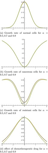
From the graphical results, we see that our results are up to expectations. We see that normal cells are the highest (see Figures 1(a) and 2(a)) at the centre of tumour site (i.e. at x = 0) and are decreasing towards the invasive ends. Similarly, tumour cells are increasing with time towards the invasive ends (refer Figures 1(b) and 2(b)). Means cancer is increasing with time. At the same time, we can see that immune cells are also increasing with respect to time (refer Figures 1(c) and 2(c)). This is a good sign to fight against cancer. The drug effect is most at the centre of tumour site (which is needed and expected too) and decreasing towards invasive ends (see Figures 1(d) and 2(d)).

Figure 1. Growth rate of different cells – 3D representation. (a) Change rate of normal cells, (b) change rate of cancerous cells,(c) change rate of immune cells and (d) effect of chemotherapeutic drug.

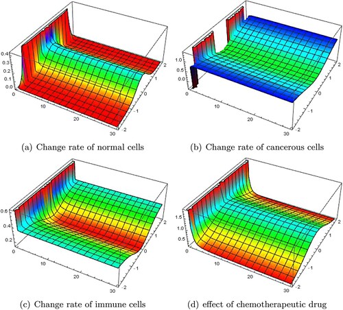
Figure 2. Growth rate of different cells- 2D representation for t = 1. (a) Growth rate of normal cells for $\alpha =0.5,0.7$ and 0.9, (b) growth rate of cancerous cells for $\alpha =0.5,0.7$ and 0.9, (c) growth rate of resistant cells for $\alpha =0.5,0.7$ and 0.9 and (d) effect of chemotherapeutic drug for $\alpha =0.5,0.7$ and 0.9.

6. Conclusion

We have concentrated on the illness model using chemotherapeutic cells using the Laplace transform and Yang–Abdel–Cattani fractional differential operator. Additionally, we have demonstrated the presence and coherence of arrangements. Additionally established are their mathematical and graphical arrangements. In the future, we can concentrate on the side effects of medication as well as alternative methods to predict disease and create strategies for the future. we can say that the tumour is increasing with respect to time but has the potential to be treated if chemotherapeutic drugs are given with prescribed dosages and at regular intervals of time. We also see that the absolute errors are decreasing with respect to time and this is a good agreement with our findings.

Acknowledgments

Manvendra Narayan Mishra led the study, interpreted results and arranged the required literature for the study, wrote the manuscript and did all the numerical calculations while A. F. Aljohani summarized the data for tables, drew the figures/graphs and created the study site map and formatted the final document. Both authors read, edited, and finalized the draft.

Disclosure statement

No potential conflict of interest was reported by the author(s).

Data availability statement

The availability of statistics is already cited in the article.

References

- Adam JA. The dynamics of growth-factor-modifiedimmune response to cancer growth: one dimensional models. Math Comput Model. 1993 Feb 1;17(3):83–106.
- Ansarizadeh F, Singh M, Richards D. Modelling of tumor cells regression in response to chemotherapeutic treatment. Appl Math Model. 2017 Aug 1;48:96–112.
- de Pillis LG, Gu W, Radunskaya AE. Mixed immunotherapy and chemotherapy of tumors: modeling, applications and biological interpretations. J Theor Biol. 2006 Feb 21;238(4):841–862.
- Fahmy S, El-Geziry AM, Mohamed E, et al. Fractional-order mathematical model for chronic myeloid leukae-mia. In: 2017 European Conference on Circuit Theory and Design (ECCTD); 2017. p. 1–4.
- Friedman A. A hierarchy of cancer models and their mathematical challenges. Discrete Contin Dyn Syst-B. 2004;4(1):147.
- Jemal A, Bray F, Center MM, et al. Global cancer statistics. CA: Cancer J Clin. 2011 Mar;61(2):69–90.
- Joshi B, Wang X, Banerjee S, et al. On immunotherapies and cancer vaccination protocols: a mathematical modelling approach. J Theor Biol. 2009 Aug 21;259(4):820–827.
- Kilbas AA, Srivastava HM, Trujillo JJ. Theory and applications of fractional differential equations. Elsevier; 2006.
- Basirzadeh H, Nazari S. T-lymphocyte cell injection cancer immunotherapy: an optimal control approach. Iran J Oper Res. 2012;3(1):46–60.
- Biemar F, Foti M. Global progress against cancer – challenges and opportunities. Cancer Biol Med. 2013 Dec;10(4):183.
- Bray F, Jemal A, Grey N, et al. Global cancer transitions according to the human development index (2008–2030): a population-based study. Lancet Oncol. 2012 Aug 1;13(8):790–801.
- Castiglione F, Piccoli B. Cancer immunotherapy, mathematical modeling and optimal control. J Theor Biol. 2007 Aug 21;247(4):723–732.
- De Pillis LG, Radunskaya A. A mathematical tumor model with immune resistance and drug therapy: an optimal control approach. Comput Math Methods Med. 2001 Jan 1;3(2):79–100.
- De Pillis LG, Radunskaya A. The dynamics of an optimally controlled tumor model: a case study. Math Comput Model. 2003 Jun 1;37(11):1221–1244.
- De Pillis LG, Radunskaya AE, Wiseman CL. A validated mathematical model of cell-mediated immune response to tumor growth. Cancer Res. 2005 Sep 1;65(17):7950–7958.
- He JH. Homotopy perturbation technique. Comput Methods Appl Mech Eng. 1999 Aug 1;178(3–4):257–262.
- Itik M, Salamci MU, Banks SP. SDRE optimal control of drug administration in cancer treatment. Turk J Electr Eng Comput Sci. 2010;18(5):715–730.
- Ku-Carrillo RA, Delgadillo SE, Chen-Charpentier BM. A mathematical model for the effect of obesity on cancer growth and on the immune system response. Appl Math Model. 2016 Apr 1;40(7–8):4908–4920.
- Morgan AP. A homotopy for solving polynomial systems. Appl Math Comput. 1986 Jan 1;18(1):87–92.
- Murray JM. Optimal control for a cancer chemotheraphy problem with general growth and loss functions. Math Biosci. 1990 Mar 1;98(2):273–287.
- Shi L, Tayebi S, Arqub OA, et al. The novel cubic B-spline method for fractional Painlevé and Bagley-Trovik equations in the Caputo, Caputo-Fabrizioand conformable fractional sense. Alex Eng J. 2022 Oct 1.
- Arqub OA, Osman MS, Abdel-Aty AH, et al. A numerical algorithm for the solutions of ABC singular Lane-Emden type models arising in astrophysics using reproducing kernel discretization method. Mathematics. 2020 Jun 5;8(6):923.
- Ali KK, Abd El Salam MA, Mohamed EM, et al. Numerical solution for generalized nonlinear fractional integro-differential equations with linear functional arguments using Chebyshev series. Adv Differ Equ. 2020 Dec;2020(1):1–23.
- Djennadi S, Shawagfeh N, Osman MS, et al. The Tikhonov regularization method for the inverse source problem of time fractional heat equation in the view of ABC-fractional technique. Phys Scr. 2021 Jun 15;96(9):Article ID 094006.
- Nanda S, Moore H, Lenhart S. Optimal control of treatment in a mathematical model of chronic myelogenous leukemia. Math Biosci. 2007 Nov 1;210(1):143–156.
- Rihan FA, Rahman DA, Lakshmanan S, et al. A time delay model of tumour-immune system interactions: global dynamics, parameter estimation, sensitivity analysis. Appl Math Comput. 2014 Apr 1;232:606–623.
- Swan GW. Role of optimal control theory in cancer chemotherapy. Math Biosci. 1990 Oct 1;101(2):237–284.
- Chaplain MA, Lolas G. Mathematical modelling of cancer cell invasion of tissue: the role of the urokinase plasminogen activation system. Math Models Methods Appl Sci. 2005 Nov;15(11):1685–1734.
- Phadtare A, Rathod C, Thonte S, et al. Problems in cancer therapy: a review. Indo Am J Pharm Res. 2013;3(3):2778–2794.
- Kuznetsov VA. Dynamics of immune processes during tumor growth; 1992.
- Kumar S, Atangana A. A numerical study of the nonlinear fractional mathematical model of tumor cells in presence of chemotherapeutic treatment. Int J Biomath. 2020 Apr 17;13(3):Article ID 2050021.
- Ganji RM, Jafari H, Moshokoa SP, et al. A mathematical model and numerical solution for brain tumor derived using fractional operator. Results Phys. 2021 Sep 1;28:Article ID 104671.
- Tuan NH, Ganji RM, Jafari H. A numerical study of fractional rheological models and fractional Newell-Whitehead-Segel equation with non-local and non-singular kernel. Chinese J Phys. 2020 Dec 1;68:308–320.
- Karthikeyan K, Karthikeyan P, Baskonus HM, et al. Almost sectorial operators on ψ-Hilfer derivative fractional impulsive integro-differential equations. Math Methods Appl Sci. 2022 Sep 15;45(13):8045–8059.
- He ZY, Abbes A, Jahanshahi H, et al. Fractional-order discrete-time SIR epidemic model with vaccination: chaos and complexity. Mathematics. 2022 Jan 6;10(2):165.
- Jin F, Qian ZS, Chu YM. On nonlinear evolution model for drinking behavior under Caputo-Fabrizio derivative. J Appl Anal Comput. 2022;12(2):790–806.
- Iqbal MA, Wang Y, Miah MM, et al. Study on date-Jimbo-Kashiwara-Miwa equation with conformable derivative dependent on time parameter to find the exact dynamic wave solutions. Fractal Fract. 2021 Dec 23;6(1):4.
- Chu YM, Bashir S, Ramzan M, et al. Model-based comparative study of magnetohydrodynamics unsteady hybrid nanofluid flow between two infinite parallel plates with particle shape effects. Math Methods Appl Sci. 2022 Mar 18.
- Khan MA, Ullah S, Kumar S. A robust study on 2019-nCOV outbreaks through non-singular derivative. Eur Phys J Plus. 2021 Feb;136(2):1–20.
- Dubey RS, Baleanu D, Mishra M, et al. Solution of modified Bergman's minimal blood glucose insulin model using Caputo-Fabrizio fractional derivative. CMES. 2021;128(3):1247–1263.
- Zhang L, Rahman MU, Ahmad S, et al. Dynamics of fractional order delay model of coronavirus disease. AIMS Math. 2022;7(3):4211–4232.
- Zhang L, Arfan M, Ali A. Investigation of mathematical model of transmission co-infection TB in HIV community with a non-singular kernel. Results Phys. 2021 Sep 1;28:Article ID 104559.
- Liu X, Arfan M, Ur Rahman M, et al. Analysis of SIQR type mathematical model under Atangana-Baleanu fractional differential operator. Comput Methods Biomech Biomed Engin. 2022 Mar;3:1–5.
- Xu C, Baleanu D. On fractional-order symmetric oscillator with offset-boosting control. Nonlinear Anal: Model Control. 2022 Jul 19;27(5):994–1008.
- Liu X, Ahmad S, Baleanu D, et al. A new fractional infectious disease model under the non-singular Mittag-Leffler derivative. Waves Random Complex Media. 2022 Feb;22:1–27.
- Rafique J, Afzal QQ, Perveen M, et al. Drug delivery of carvedilol (cardiovascular drug) using phosphorene as a drug carrier: a DFT study. J Taibah Univ Sci. 2022 Dec 31;16(1):31–46.
- Alarabi TH, Elgazery NS, Elelamy AF. Mathematical model of oxytactic bacteria's role on MHD nanofluid flow across a circular cylinder: application of drug-carrier in hypoxic tumour. J Taibah Univ Sci. 2022 Dec 31;16(1):703–724.
- Alshehri MH, Duraihem FZ, Alalyani A, et al. A Caputo (discretization) fractional-order model of glucose-insulin interaction: numerical solution and comparisons with experimental data. J Taibah Univ Sci. 2021 Jan 1;15(1):26–36.
- Shrahili M, Dubey RS, Shafay A. Inclusion of fading memory to Banister model of changes in physical condition. Discrete Contin Dyn Syst-S. 2020;13(3):881.
- Malyk IV, Gorbatenko M, Chaudhary A, et al. Numerical solution of nonlinear fractional diffusion equation in framework of the Yang-Abdel-Cattani derivative operator. Fractal Fract. 2021 Jul 2;5(3):64.
- Gill V, Dubey RS. New analytical method for Klein-Gordon equations arising in quantum field theory. European J Adv Eng Technol. 2018;5(8):649–655.
- Dubey RS, Goswami P. Mathematical model of diabetes and its complication involving fractional operator without singular kernal. Discrete Contin Dyn Syst-S. 2021;14(7):2151.
- Jleli M, Kumar S, Kumar R, et al. Analytical approach for time fractional wave equations in the sense of Yang-Abdel-Aty-Cattani via the homotopy perturbation transform method. Alex Eng J. 2020 Oct 1;59(5):2859–2863.
- Prabhakar TR. A singular integral equation with a generalized Mittag Leffler function in the kernel; 1971.
- Dubey RS, Mishra MN, Goswami P. Effect of covid-19 in India – a prediction through mathematical modeling using Atangana Baleanu fractional derivative. J Interdiscip Math. 2022 May;11:1–4.
- Yang XJ, Abdel-Aty M, Cattani C. A new general fractional-order derivative with Rabotnov fractional-exponential kernel applied to model the anomalous heat transfer. Therm Sci. 2019;23(3 Part A):1677–1681.
- Yang XJ, Baleanu D, Srivastava HM. Local fractional integral transforms and their applications. Academic Press; 2015.